


1. Introduction
The problem of finding upper bounds or approximations for ruin probabilities is a classic one. The literature on it is vast, and it probably starts with the celebrated paper [Reference Lundberg18]. It considered the wealth of an insurance company described by a linear drift (modelling the incoming premiums) and a compound Poisson distribution (modelling the incoming claims). The famous Lundberg inequality now gives an upper bound for the probability that the wealth of the company will eventually fall below zero. A crucial assumption for this inequality is the so-called ‘small claim assumption’, i.e. we have to assume, roughly speaking, that the distribution of the claims has exponential moments.
The generalizations of this basic model are numerous. Two major directions could be described as follows. On the one hand, we can try to model the incoming claims and the premiums in a more complicated way, for example allowing claims with heavy tails [Reference Embrechts and Veraverbeke6], or replacing the compensated compound Poisson process by a general Lévy process [Reference Klüppelberg, Kyprianou and Maller15].
The second direction would be to allow insurance companies a business different from the basic model of incoming premiums and claims that have to be paid. This could be reinsurance contracts with other insurance companies [Reference Schmidli23] or the possibility to invest in the stock market [Reference Gaier, Grandits and Schachermayer8]. Inherent with these two generalizations are optimization problems, namely how to reinsure or how to invest in such a way that the ultimate ruin is minimized.
In contrast to the one-dimensional situation (i.e. we consider only one wealth process), the literature on the multidimensional case is not that huge. Let us mention just two articles. The first one considers large-deviation results for the probability that a multidimensional process hits a certain set [Reference Collamore5]. The second one, [Reference Avram, Palmowski and Pistorius4], studies the joint ruin problem for two insurance companies that divide between them both claims and premiums in some specified proportions (modelling two branches of the same insurance company or an insurance and reinsurance company). Finally, for an excellent overview on the topic of ruin probabilities, see [Reference Asmussen and Albrecher3].
In this paper we consider the following two-dimensional controlled ruin problem. Let us denote the wealth of two companies by
 $(X_t)_{t\geq 0}$
and
$(X_t)_{t\geq 0}$
and
 $(Y_t)_{t\geq 0}$
, and the corresponding two-dimensional state process by
$(Y_t)_{t\geq 0}$
, and the corresponding two-dimensional state process by
 $(Z_t)_{t\geq 0}$
, i.e.
$(Z_t)_{t\geq 0}$
, i.e.
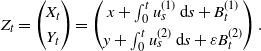 \begin{equation} Z_t = \begin{pmatrix} X_t \\[3pt] Y_t \end{pmatrix} = \begin{pmatrix} x + \int_0^t u^{(1)}_s\,{\mathrm{d}} s + B^{(1)}_t \\[3pt] y + \int_0^t u^{(2)}_s\,{\mathrm{d}} s + \varepsilon B^{(2)}_t \end{pmatrix}.\end{equation}
Here,
 $(x,y)\,=\!:\,z$
denotes the initial endowment of the companies,
$(x,y)\,=\!:\,z$
denotes the initial endowment of the companies,
 $B^{(1)}$
and
$B^{(1)}$
and
 $B^{(2)}$
are independent standard Brownian motions, and
$B^{(2)}$
are independent standard Brownian motions, and
 $u^{(1)}$
and
$u^{(1)}$
and
 $u^{(2)}$
are our control processes. We write G for the positive quadrant, i.e.
$u^{(2)}$
are our control processes. We write G for the positive quadrant, i.e.
 $G\,:\!=\,\{(x,y)\mid x \gt 0,y \gt 0\}$
, and
$G\,:\!=\,\{(x,y)\mid x \gt 0,y \gt 0\}$
, and
 $\varepsilon$
denotes a small positive constant. Moreover, we define the ruin time
$\varepsilon$
denotes a small positive constant. Moreover, we define the ruin time
 $\tau=\inf\{t \gt 0 \mid Z_t \notin G\}$
, i.e. the first time at which one of the two companies is ruined. Finally, we define the set of admissible strategies u as
$\tau=\inf\{t \gt 0 \mid Z_t \notin G\}$
, i.e. the first time at which one of the two companies is ruined. Finally, we define the set of admissible strategies u as
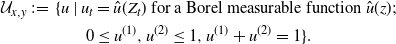 \begin{align} {\mathcal U}_{x,y} \,:\!=\, \{u & \mid u_t = \hat{u}(Z_t)\mbox{ for a Borel measurable function }\hat{u}(z); \nonumber \\ & \quad 0 \leq u^{(1)},u^{(2)} \leq 1, u^{(1)}+u^{(2)} =1\}. \end{align}
Remark 1. Note that the SDE (1) with
 $u \in {\mathcal U}_{x,y}$
has a unique strong solution by [Reference Veretennikov24], since we have Borel measurability and boundedness for the drift coefficient (see also [Reference Karatzas and Shreve14, Note 5.10]). Our aim is to maximize the target functional given by
$u \in {\mathcal U}_{x,y}$
has a unique strong solution by [Reference Veretennikov24], since we have Borel measurability and boundedness for the drift coefficient (see also [Reference Karatzas and Shreve14, Note 5.10]). Our aim is to maximize the target functional given by
 \begin{equation}J(x,y,u)=\mathbb{P}_{x,y}(\tau(u) = \infty) \to \max,\end{equation}
i.e. the probability that both companies survive should be maximized.
Let us mention two interpretations of this problem. The first, given in [Reference McKean and Shepp19], is that a government can influence the drift of the companies by a certain tax policy, but the total amount of ‘support’ is bounded by the condition that the sum of the drifts is one. For the second interpretation, write the drift vector as
 $\small \bigg(\begin{array}{c}1/2 +\hat{u}_t \\ 1/2-\hat{u}_t \end{array}\bigg)$
(here,
$\small \bigg(\begin{array}{c}1/2 +\hat{u}_t \\ 1/2-\hat{u}_t \end{array}\bigg)$
(here,
 $\hat{u}_t$
denotes transfer payments from one company to the other); we can imagine two companies collaborating with the goal that both want to survive. Collaborating companies have been considered in insurance mathematics, e.g. in [Reference Albrecher, Azcue and Muler2,Reference Grandits10], where the goal is to maximize dividends.
$\hat{u}_t$
denotes transfer payments from one company to the other); we can imagine two companies collaborating with the goal that both want to survive. Collaborating companies have been considered in insurance mathematics, e.g. in [Reference Albrecher, Azcue and Muler2,Reference Grandits10], where the goal is to maximize dividends.
Another point of view was given in [Reference Gu, Steffensen and Zheng13]. We could think of two business lines within one company rather than two cooperating companies, e.g. life and non-life insurance in an insurance company. The manager of the whole company can allocate capital to the two business lines in order to serve a given objective, in our case to keep both business lines solvent, and in the case of [Reference Gu, Steffensen and Zheng13] to maximize the expected dividends. As noted in [Reference Gu, Steffensen and Zheng13], this is a realistic setup and capital allocation is an important management discipline nowadays.
Now, it is quite possible that one of the two business lines faces some small volatility in comparison to the other. A first example would be, as mentioned above, life and non-life insurance business. The first one relies heavily on mortality tables, which allow the prediction of claims that have to be paid in the future in quite a precise manner. This clearly provides a small volatility in comparison to business lines handling, say, natural disasters like storms and earthquakes. An empirical study in this direction can be found in [Reference Palau22]: CNP Assurances SA, one of the biggest French life insurance companies, has a volatility of 3.98 (see [Reference Palau22, Table 2]), and German Allianz SE, which covers both life and non-life business, has a value of 48.8.
A second example would be operational risk (which has some similarities to insurance risk [Reference McNeil, Frey and Embrechts20, Section 10]) in comparison to market risk for a bank [Reference Li, Zhu, Lee, Wu, Feng and Shi17, Figure 6 and Table 3], where we find respective volatility values of 0.07 and 0.49. In all these cases, the result of our paper would provide information as to when it is appropriate for a general manager to transfer money from one business to the other if the goal is to keep both solvent.
In [Reference McKean and Shepp19] the problem is solved for the case
 $\varepsilon=1$
. The authors show that it is optimal to give the whole drift to the company that has a smaller endowment at the moment considered. It is also mentioned there that the case of different volatilities is open. For convenience, in our paper we set one of the two volatilities equal to 1 and consider the case where the second company faces a small volatility in comparison to the first.
$\varepsilon=1$
. The authors show that it is optimal to give the whole drift to the company that has a smaller endowment at the moment considered. It is also mentioned there that the case of different volatilities is open. For convenience, in our paper we set one of the two volatilities equal to 1 and consider the case where the second company faces a small volatility in comparison to the first.
The goal of our paper is to find an admissible strategy that produces a target functional that is a uniform approximation of the value function V(x,y) in
 $\overline{G} \,:\!=\, \mathbf{R}_0^+ \times \mathbf{R}_0^+$
. Our method will be the following:
$\overline{G} \,:\!=\, \mathbf{R}_0^+ \times \mathbf{R}_0^+$
. Our method will be the following:
-
(i) Find an approximation for V(x,y), say
 $\tilde{V}(x,y)$
, by formal methods of singular perturbation theory.
$\tilde{V}(x,y)$
, by formal methods of singular perturbation theory. -
(ii) Show the validity of the approximation, i.e. that
$|V(x,y)-\tilde{V}(x,y)|=o(1)$
for
$\varepsilon \to 0$
uniformly in
$\overline{G}$
. -
(iii) For the difference considered in (ii) we shall need a kind of Alexandrov–Bakelman–Pucci (ABP) estimate. In comparison to standard results (see, e.g., [Reference Gilbarg and Trudinger9]), we have to deal with two special features: first, we have an unbounded domain, and second, we need some control over the constant on the right-hand side of the ABP estimate; more precisely, we have to control its dependence on
$\varepsilon$
. The reason for this is that we want to conclude from the smallness of the inhomogeneity of a partial differential equation (PDE) for
$D\,:\!=\,\tilde{V}-V$
that (ii) is indeed true. A result of this kind is proved in [Reference Grandits12], and we shall use it. -
(iv) It turns out that we can easily find a strategy
$\tilde{u}$
that produces
$\tilde{V}(x,y)$
as target functional. Unfortunately,
$\tilde{u}$
is not an admissible strategy. So, in a final step we construct an admissible strategy
$\hat{u}$
with corresponding target functional
$\hat{V}(x,y)$
that fulfills
$|\hat{V}(x,y)-\tilde{V}(x,y)|=o(1)$
for
$\varepsilon\to 0$
uniformly in
$\overline{G}$
, which, together with (ii), gives the final result
$|\hat{V}(x,y)-V(x,y)|=o(1)$
for
$\varepsilon\to 0$
uniformly in
$\overline{G}$
.


In Section 2 we give a preliminary result, which can be taken from [Reference Grandits11] where a similar problem is considered. More precisely, we have the same state process in the present paper, but the target functional is different. Namely, the goal in [Reference Grandits11] is to maximize the expectation of the number of surviving companies. This produces the same Hamilton–Jacobi–Bellman (HJB) equation, but with non-homogeneous boundary conditions. In Section 3 we deal with the formal approximation of (i). Finally, in Section 4 we formulate the ABP estimate of (iii) and apply it in order to get (ii) and (iv).
2. A preliminary result
Let
 $V(x,y) \,:\!=\, \sup_{u \in {\mathcal U}_{x,y}} J(x,y,u)$
be the value function of our problem. Then the following proposition shows that V(x,y) is a classical solution of the HJB equation of the problem.
$V(x,y) \,:\!=\, \sup_{u \in {\mathcal U}_{x,y}} J(x,y,u)$
be the value function of our problem. Then the following proposition shows that V(x,y) is a classical solution of the HJB equation of the problem.
Proposition 1.
V(x,y) is the unique classical (i.e.
 $V \in C(\overline{G})$
,
$V \in C(\overline{G})$
,
 $V_{xx},V_{xy},V_{yy} \in C^2(G)$
) solution of the problem
$V_{xx},V_{xy},V_{yy} \in C^2(G)$
) solution of the problem
 \begin{equation*} {\mathcal L}V \,:\!=\, \max \{V_x,V_y\}+\tfrac{1}{2}\Delta^{(\epsilon)} V=0\mbox{ on } G, \quad V(x,0) = V(0,y) = 0, \quad \lim_{x\to \infty,y\to \infty}V(x,y)= 1, \end{equation*}
where we have used the notation
 $\Delta^{(\epsilon)} \,:\!=\, ({\partial^2}/{\partial x^2})+\varepsilon^2({\partial^2}/{\partial y^2})$
, and
$\Delta^{(\epsilon)} \,:\!=\, ({\partial^2}/{\partial x^2})+\varepsilon^2({\partial^2}/{\partial y^2})$
, and
 $\lim_{x\to \infty,y\to \infty}$
, here and in what follows, is understood along arbitrary sequences in the plane. Additionally, we have
$\lim_{x\to \infty,y\to \infty}$
, here and in what follows, is understood along arbitrary sequences in the plane. Additionally, we have
 $V_{xx},V_{xy},V_{yy} \in C(\overline{G} \setminus \{(0,0)\})$
.
$V_{xx},V_{xy},V_{yy} \in C(\overline{G} \setminus \{(0,0)\})$
.
Proof. The proof works analogously to the proofs of [Reference Grandits11, Theorem 3.1, Propositions 3.1 and 3.2], with
 $w=(1-\mathrm{e}^{-2x})(1-e^{-{2y}/{\varepsilon^2}})$
instead of
$w=(1-\mathrm{e}^{-2x})(1-e^{-{2y}/{\varepsilon^2}})$
instead of
 $w=2-\mathrm{e}^{-2x}-\mathrm{e}^{-2y}$
, and
$w=2-\mathrm{e}^{-2x}-\mathrm{e}^{-2y}$
, and
 $v=1-\mathrm{e}^{-x}-\mathrm{e}^{-y/\varepsilon^2}$
instead of
$v=1-\mathrm{e}^{-x}-\mathrm{e}^{-y/\varepsilon^2}$
instead of
 $v=2-\mathrm{e}^{-x}-\mathrm{e}^{-y}$
. The fact that we have
$v=2-\mathrm{e}^{-x}-\mathrm{e}^{-y}$
. The fact that we have
 $\varepsilon=1$
there does not cause any harm, and the homogeneous boundary conditions at
$\varepsilon=1$
there does not cause any harm, and the homogeneous boundary conditions at
 $\{(x,0)\mid x \geq 0\}$
and
$\{(x,0)\mid x \geq 0\}$
and
 $\{(0,y)\mid y \geq 0\}$
in our case sometimes make life even easier.
$\{(0,y)\mid y \geq 0\}$
in our case sometimes make life even easier.
3. Heuristics: A formal approximation
Let us first consider the case
 $\varepsilon =0$
. In this case the strategy
$\varepsilon =0$
. In this case the strategy
 $u\,:\!=\, \small{\bigg(\begin{array}{c}1 \\ 0 \end{array}\bigg)}$
is clearly optimal, since in this case company Y does not face any risk. Indeed, the volatility of its wealth process is zero, and the drift non-negative. Therefore, all the drift should be given to
$u\,:\!=\, \small{\bigg(\begin{array}{c}1 \\ 0 \end{array}\bigg)}$
is clearly optimal, since in this case company Y does not face any risk. Indeed, the volatility of its wealth process is zero, and the drift non-negative. Therefore, all the drift should be given to
 $X_t$
. This leads to the target functional
$X_t$
. This leads to the target functional
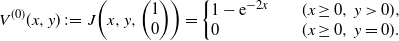 \[ V^{(0)}(x,y)\,:\!=\,J\bigg(x,y,\bigg(\begin{array}{c}1 \\ 0 \end{array}\bigg)\bigg) = \left\{ \begin{array}{l@{\qquad}l} 1-\mathrm{e}^{-2x} & (x \geq 0,\,y \gt 0), \\ 0 & (x \geq 0,\,y=0). \end{array} \right.\]
By the Barles/Bertham procedure (see, e.g., [Reference Fleming and Soner7, Chapter VII]), we can show that
 $V^{(0)}$
will be an approximation of V(x,y) in compact subsets of G. But since
$V^{(0)}$
will be an approximation of V(x,y) in compact subsets of G. But since
 $V^{(0)}(x,y)$
is discontinuous at the positive x-axis, it can never be a uniform approximation of our continuous value function on
$V^{(0)}(x,y)$
is discontinuous at the positive x-axis, it can never be a uniform approximation of our continuous value function on
 $\overline{G}$
. One goal of this paper is to provide such a uniform approximation.
$\overline{G}$
. One goal of this paper is to provide such a uniform approximation.
Taking a look at the case
 $\varepsilon=1$
, where an explicit solution is given in [Reference McKean and Shepp19], we expect that
$\varepsilon=1$
, where an explicit solution is given in [Reference McKean and Shepp19], we expect that
 $\overline{G}$
splits into two simply connected regions P and N, with
$\overline{G}$
splits into two simply connected regions P and N, with
 \begin{equation*} P \,:\!=\, \{(x,y) \in \overline{G} \mid V_x(x,y) \geq V_y(x,y)\}, \qquad N \,:\!=\, \{(x,y) \in \overline{G} \mid V_x(x,y) \lt V_y(x,y)\}.\end{equation*}
This means that we assign the full drift of one in region P to the X company, and in region N to the Y company. Since
 $\varepsilon$
is small, and hence the risk of ruin for the second companyis small, we expect that the region N is very thin. The separation curve, starting from the origin, is denoted by
$\varepsilon$
is small, and hence the risk of ruin for the second companyis small, we expect that the region N is very thin. The separation curve, starting from the origin, is denoted by
 $A\,:\!=\,\{(x,y) \in \overline{G} \mid V_x(x,y) = V_y(x,y)\}$
.
$A\,:\!=\,\{(x,y) \in \overline{G} \mid V_x(x,y) = V_y(x,y)\}$
.
Remark 2. We can easily check that
 $\{(0,y)\mid y \gt 0\} \subset P$
. Indeed, we have
$\{(0,y)\mid y \gt 0\} \subset P$
. Indeed, we have
 $V_y(0,y)=0$
and
$V_y(0,y)=0$
and
 $V_x(0,y) \gt 0$
. The latter inequality can be verified as follows:
$V_x(0,y) \gt 0$
. The latter inequality can be verified as follows:
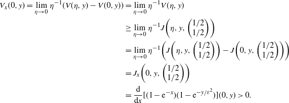 \begin{align*} V_x(0,y) = \lim_{\eta \to 0}\eta^{-1}(V(\eta,y)-V(0,y)) & = \lim_{\eta \to 0}\eta^{-1}V(\eta,y) \\ & \geq \lim_{\eta \to 0}\eta^{-1}J\bigg(\eta,y,\bigg(\begin{array}{c}1/2 \\ 1/2 \end{array}\bigg)\bigg) \\ & = \lim_{\eta \to 0}\eta^{-1}\bigg(J\bigg(\eta,y,\bigg(\begin{array}{c}1/2 \\ 1/2\end{array}\bigg)\bigg) - J\bigg(0,y,\bigg(\begin{array}{c}1/2 \\ 1/2\end{array}\bigg)\bigg)\bigg) \\ & = J_x\bigg(0,y,\bigg(\begin{array}{c}1/2 \\ 1/2\end{array}\bigg)\bigg) \\ & = \frac{{\mathrm{d}}}{{\mathrm{d}} x}[(1-\mathrm{e}^{-x})(1-{\mathrm{e}}^{-y/ \varepsilon^2})](0,y) \gt 0. \end{align*}
By similar arguments we have
 $\{(x,0)\mid x \gt 0\} \subset N$
, which suggests that the separation curve starts at the origin.
$\{(x,0)\mid x \gt 0\} \subset N$
, which suggests that the separation curve starts at the origin.
Moreover, we expect that V has a layer behavior in region N, i.e. we expect the existence of a ‘fast variable’.
We now explain the following concepts from singular perturbation theory. A (solution) function, say
 $u(z,\varepsilon)$
, has a regular approximation if we can approximate it on the whole domain by a sum
$u(z,\varepsilon)$
, has a regular approximation if we can approximate it on the whole domain by a sum
 $\sum_{n=0}^m\delta_n(\varepsilon)\phi(z)$
, with
$\sum_{n=0}^m\delta_n(\varepsilon)\phi(z)$
, with
 $\delta_{n+1}=o(\delta_n)$
[Reference Meyer and Parter21, Section 3]. A first-order approximation would be, in our case, a function depending only on z. Usually, differential equations with a small parameter in front of one of the derivatives of highest order do not possess regular expansions, since these functions fail in general to fulfill some of the conditions imposed on the solution, e.g. boundary conditions. This leads to the so-called layer behavior, or the existence of a fast variable, near the critical manifold. To find this variable, we start from the ansatz
$\delta_{n+1}=o(\delta_n)$
[Reference Meyer and Parter21, Section 3]. A first-order approximation would be, in our case, a function depending only on z. Usually, differential equations with a small parameter in front of one of the derivatives of highest order do not possess regular expansions, since these functions fail in general to fulfill some of the conditions imposed on the solution, e.g. boundary conditions. This leads to the so-called layer behavior, or the existence of a fast variable, near the critical manifold. To find this variable, we start from the ansatz
 $q\,:\!=\,{y}/{\varepsilon^\alpha}$
; we want to find the significant degeneration of the PDE in region N. Denoting V in region N by
$q\,:\!=\,{y}/{\varepsilon^\alpha}$
; we want to find the significant degeneration of the PDE in region N. Denoting V in region N by
 $V^{(N)}$
, we get the following PDE in region N:
$V^{(N)}$
, we get the following PDE in region N:
 $V^{(N)}_y+\frac{1}{2}\Delta^{(\epsilon)} V^{(N)}=0$
. Transforming to the variables (x,q) yields, with
$V^{(N)}_y+\frac{1}{2}\Delta^{(\epsilon)} V^{(N)}=0$
. Transforming to the variables (x,q) yields, with
 $\bar{V}^{(N)}(x,q)=V^{(N)}(x,\varepsilon^\alpha q)$
,
$\bar{V}^{(N)}(x,q)=V^{(N)}(x,\varepsilon^\alpha q)$
,
 \[ \varepsilon^{-\alpha} \bar{V}^{(N)}_q+\frac{1}{2} \bar{V}^{(N)}_{xx}+\frac{\varepsilon^{2-2\alpha}}{2} \bar{V}^{(N)}_{qq}=0,\]
which, after multiplying by
 $\varepsilon^2$
and with
$\varepsilon^2$
and with
 $\varepsilon\to 0$
, gives the significant degeneration for
$\varepsilon\to 0$
, gives the significant degeneration for
 $\alpha=2$
, i.e.
$\alpha=2$
, i.e.
 \begin{equation} \bar{V}^{(N)}_q+\frac{1}{2} \bar{V}^{(N)}_{qq}=0.\end{equation}
Let us comment briefly on the concept of a significant degeneration [Reference Meyer and Parter21, Section 4]. A significant degeneration of a differential operator is a degeneration which is not contained in another degeneration. By ‘degeneration’ we mean expressing the operator in the new variable and, after renorming such that the biggest term is O(1), letting
 $\varepsilon$
tend to zero. In our example this would give, if we take, e.g.,
$\varepsilon$
tend to zero. In our example this would give, if we take, e.g.,
 $\alpha=1$
,
$\alpha=1$
,
 $\bar{V}^{(N)}_q=0$
, a degeneration that we could get if we started from (4); hence, the degeneration for
$\bar{V}^{(N)}_q=0$
, a degeneration that we could get if we started from (4); hence, the degeneration for
 $\alpha=1$
is contained in the one for
$\alpha=1$
is contained in the one for
 $\alpha=2$
. Similarly, we find, for
$\alpha=2$
. Similarly, we find, for
 $\alpha=3$
,
$\alpha=3$
,
 $\frac{1}{2} \bar{V}^{(N)}_{qq}=0$
, again contained in the case
$\frac{1}{2} \bar{V}^{(N)}_{qq}=0$
, again contained in the case
 $\alpha=2$
. We can easily check that the degeneration for
$\alpha=2$
. We can easily check that the degeneration for
 $\alpha=2$
is not contained in another one, and is therefore significant. By the ‘heuristic principle’ formulated in [Reference Meyer and Parter21, Section 4], ‘boundary layer variables’ or ‘fast variables’ correspond to significant degenerations. We give more details on this procedure in Section 5 for the one-dimensional example provided in the Appendix.
$\alpha=2$
is not contained in another one, and is therefore significant. By the ‘heuristic principle’ formulated in [Reference Meyer and Parter21, Section 4], ‘boundary layer variables’ or ‘fast variables’ correspond to significant degenerations. We give more details on this procedure in Section 5 for the one-dimensional example provided in the Appendix.
Solving (4), we arrive at
 $\bar{V}^{(N)}(x,q)=C(x)+D(x)\mathrm{e}^{-2q}$
, and therefore, using the boundary condition
$\bar{V}^{(N)}(x,q)=C(x)+D(x)\mathrm{e}^{-2q}$
, and therefore, using the boundary condition
 $\bar{V}^{(N)}(x,0)=0$
,
$\bar{V}^{(N)}(x,0)=0$
,
 \begin{equation} \bar{V}^{(N)}(x,q) = D(x)(1-\mathrm{e}^{-2q}), \quad \mbox{or} \quad V^{(N)}(x,y) = D(x)(1-\mathrm{e}^{-{2y}/{\varepsilon^2}}).\end{equation}
We now employ the ‘boundary condition’
 $V^{(N)}(\infty,\infty)=1$
. Note that we assume here that the separation curve A generates a set N which includes points (x,y) with arbitrarily large x and y. This will be verified a posteriori. We find that
$V^{(N)}(\infty,\infty)=1$
. Note that we assume here that the separation curve A generates a set N which includes points (x,y) with arbitrarily large x and y. This will be verified a posteriori. We find that
 \begin{equation} D(\infty)=1.\end{equation}
We now assume that the curve A is described by the function
 $\phi(x)$
,
$\phi(x)$
,
 $x \in [0,\infty)$
. Since we have to change the strategy at this curve, we find the condition
$x \in [0,\infty)$
. Since we have to change the strategy at this curve, we find the condition
 \begin{equation} V^{(N)}_x(x,\phi(x))=V^{(N)}_y(x,\phi(x)).\end{equation}
Using (5) and the scaled function
 $\tilde{\phi}(x)={\phi(x)}/{\varepsilon^2}$
finally gives
$\tilde{\phi}(x)={\phi(x)}/{\varepsilon^2}$
finally gives
 \begin{equation} \frac{D^{\prime}(x)}{D(x)} = \frac{2}{\varepsilon^2}\frac{\mathrm{e}^{-2\tilde{\phi}(x)}}{1-\mathrm{e}^{-2\tilde{\phi}(x)}}.\end{equation}
We now try to construct an approximation in region P and consider the so-called ‘reduced equation’ (i.e. setting
 $\varepsilon =0$
). As previously mentioned, in this case the strategy (1,0) is optimal, and we find
$\varepsilon =0$
). As previously mentioned, in this case the strategy (1,0) is optimal, and we find
 $V^{(P)}_x+\frac{1}{2}V^{(P)}_{xx}=0$
on P, which gives, using the boundary condition
$V^{(P)}_x+\frac{1}{2}V^{(P)}_{xx}=0$
on P, which gives, using the boundary condition
 $V^{(P)}(0,y)=0$
,
$V^{(P)}(0,y)=0$
,
 \begin{equation} V^{(P)}(x,y)=F(y)(1-\mathrm{e}^{-2x}).\end{equation}
The boundary condition
 $V^{(P)}(x,\infty)=1-\mathrm{e}^{-2x}$
, which is motivated by the fact that
$V^{(P)}(x,\infty)=1-\mathrm{e}^{-2x}$
, which is motivated by the fact that
 $\sup_u \mathbb{P}_{x,\infty}(\tau(u)=\infty) = \mathbb{P}_x(\tau_X=\infty)$
, where
$\sup_u \mathbb{P}_{x,\infty}(\tau(u)=\infty) = \mathbb{P}_x(\tau_X=\infty)$
, where
 $\tau_X\,:\!=\,\inf\{t\geq 0 \mid x+t+B_t^{(1)}\leq 0\}$
, additionally provides
$\tau_X\,:\!=\,\inf\{t\geq 0 \mid x+t+B_t^{(1)}\leq 0\}$
, additionally provides
 $F(\infty)=1$
. Analogously to (7), we impose
$F(\infty)=1$
. Analogously to (7), we impose
 \begin{equation} V^{(P)}_x(x,\phi(x))=V^{(P)}_y(x,\phi(x)).\end{equation}
Hence, using (9),
 \begin{equation} \frac{F^{\prime}(\phi(x))}{F(\phi(x))}=\frac{2\mathrm{e}^{-2x}}{1-\mathrm{e}^{-2x}}.\end{equation}
Clearly, we should have
 $V^{(P)}(x,\phi(x))=V^{(N)}(x,\phi(x))$
, giving
$V^{(P)}(x,\phi(x))=V^{(N)}(x,\phi(x))$
, giving
 \begin{equation} D(x)\big(1-\mathrm{e}^{-2\tilde{\phi}(x)}\big) = F(\phi(x))(1-\mathrm{e}^{-2x}).\end{equation}
Our final ‘matching condition’ is
 $V^{(P)}_x(x,\phi(x))=V^{(N)}_x(x,\phi(x))$
, which, together with (7) and (10), means that we want continuous partial derivatives over the curve A. Finally, this gives
$V^{(P)}_x(x,\phi(x))=V^{(N)}_x(x,\phi(x))$
, which, together with (7) and (10), means that we want continuous partial derivatives over the curve A. Finally, this gives
 \begin{equation} \frac{D^{\prime}(x)}{F(\phi(x))} = \frac{2\mathrm{e}^{-2x}}{1-\mathrm{e}^{-2\tilde{\phi}(x)}}.\end{equation}
We now want to calculate the functions
 $\phi(x)$
, D(x), and F(y) from the matching conditions (8), (11)–(13).
$\phi(x)$
, D(x), and F(y) from the matching conditions (8), (11)–(13).
We start with the derivation of (12) with respect to x, giving
 \[ D^{\prime}(x)\big(1-\mathrm{e}^{-2\tilde{\phi}(x)}\big) + 2D(x)\mathrm{e}^{-2\tilde{\phi}(x)}\tilde{\phi}^{\prime}(x) = F^{\prime}(\phi(x))\phi^{\prime}(x)(1-\mathrm{e}^{-2x}) + 2F(\phi(x))\mathrm{e}^{-2x}.\]
Using (11)–(13), and dividing this equation by
 $F(\phi(x))$
, provides, after some elementary calculations,
$F(\phi(x))$
, provides, after some elementary calculations,
 \begin{equation} \frac{\mathrm{e}^{-2x}\varepsilon^2}{1-\mathrm{e}^{-2x}}=\frac{\mathrm{e}^{-2\tilde{\phi}(x)}}{1-\mathrm{e}^{-2\tilde{\phi}(x)}},\end{equation}
and, finally, the formula for the separation curve:
 \begin{equation} \tilde{\phi}(x)=\frac{1}{2}\ln\bigg(1+\frac{\mathrm{e}^{2x}-1}{\varepsilon^2}\bigg).\end{equation}
It remains to determine the functions D(x) and F(y). Plugging (15) (resp. (14)) into (8) yields
 \[ \frac{D^{\prime}(x)}{D(x)}=\frac{2\mathrm{e}^{-2x}}{1-\mathrm{e}^{-2x}}.\]
Integrating this ordinary differential equation (ODE) using the condition in (6) gives
 \begin{equation} D(x)=1-\mathrm{e}^{-2x}.\end{equation}
 \[ F(\phi(x)) = \frac{D(x)\big(1-\mathrm{e}^{-2\tilde{\phi}(x)}\big)}{1-\mathrm{e}^{-2x}} = 1-\mathrm{e}^{-2\tilde{\phi}(x)}.\]
Since
 $\phi(x)$
is bijective from
$\phi(x)$
is bijective from
 $\mathbf{R}^+_0$
to
$\mathbf{R}^+_0$
to
 $\mathbf{R}^+_0$
, we get
$\mathbf{R}^+_0$
, we get
 $F(y)=1-\mathrm{e}^{-{2y}/{\varepsilon^2}}$
. So, summarizing the results of our heuristic procedure, we find the approximations
$F(y)=1-\mathrm{e}^{-{2y}/{\varepsilon^2}}$
. So, summarizing the results of our heuristic procedure, we find the approximations
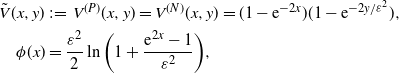 \begin{equation} \begin{aligned} \tilde{V}(x,y) & \,:\!=\, V^{(P)}(x,y)=V^{(N)}(x,y) = (1-\mathrm{e}^{-2x})(1-\mathrm{e}^{-{2y}/{\varepsilon^2}}), \\ \phi(x) & = \frac{\varepsilon^2}{2}\ln\bigg(1+\frac{\mathrm{e}^{2x}-1}{\varepsilon^2}\bigg), \end{aligned}\end{equation}
and we note again that on the separation curve
 $(x,\phi(x))$
we have
$(x,\phi(x))$
we have
 $\tilde{V}_x=\tilde{V}_y$
. Figure 1 shows a plot of the separation curve.
$\tilde{V}_x=\tilde{V}_y$
. Figure 1 shows a plot of the separation curve.
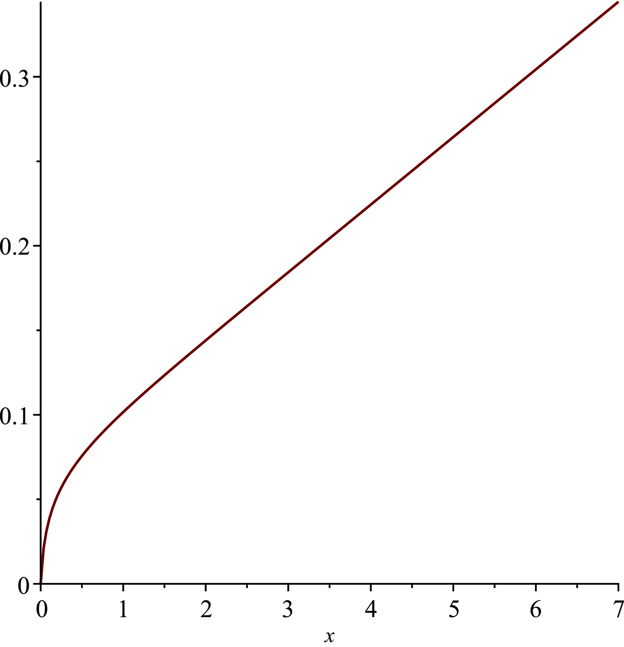
Figure 1. Plot of the separation curve
 $(x,\phi(x))$
for
$(x,\phi(x))$
for
 $\varepsilon=0.2$
.
$\varepsilon=0.2$
.
As we want to show finally that
 $\tilde{V}$
is a uniform approximation of the value function V in
$\tilde{V}$
is a uniform approximation of the value function V in
 $\overline{G}$
, we prove as a preparatory result that
$\overline{G}$
, we prove as a preparatory result that
 $\tilde{V}$
produces a small residuum in the sense of
$\tilde{V}$
produces a small residuum in the sense of
 $L^p$
,
$L^p$
,
 $p=1,2$
, if we plug it into the operator
$p=1,2$
, if we plug it into the operator
 ${\mathcal L}$
.
${\mathcal L}$
.
Lemma 1.
 ${\mathcal L}\tilde{V}=\max\big\{\tilde{V}_x,\tilde{V}_y\big\} + \frac{1}{2}\Delta^{(\epsilon)}\tilde{V}\,=\!:\,R$
on G, with
${\mathcal L}\tilde{V}=\max\big\{\tilde{V}_x,\tilde{V}_y\big\} + \frac{1}{2}\Delta^{(\epsilon)}\tilde{V}\,=\!:\,R$
on G, with
 $||R||_{L^p(G)} \leq C\varepsilon^2(-\ln\varepsilon)$
,
$||R||_{L^p(G)} \leq C\varepsilon^2(-\ln\varepsilon)$
,
 $p=1,2$
, for small
$p=1,2$
, for small
 $\varepsilon$
, a positive constant C, not depending on
$\varepsilon$
, a positive constant C, not depending on
 $\varepsilon$
, and
$\varepsilon$
, and
 $R \in L^\infty(G)$
.
$R \in L^\infty(G)$
.
Remark 3. Note that the
 $L^\infty$
-norm of R does depend on
$L^\infty$
-norm of R does depend on
 $\varepsilon$
, but since the crucial estimate that we shall use (see Theorem 1) depends only on the
$\varepsilon$
, but since the crucial estimate that we shall use (see Theorem 1) depends only on the
 $L^1$
and
$L^1$
and
 $L^2$
norms of R (there f), this will not affect the results of the paper.
$L^2$
norms of R (there f), this will not affect the results of the paper.
Proof. An elementary calculation provides
 \begin{equation*} {\mathcal L}\tilde{V}(x,y) = \mathbf{1}_{\{y\geq\phi(x)\}}\frac{2}{\varepsilon^2}(\mathrm{e}^{-2x}-1)\mathrm{e}^{-{2y}/{\varepsilon^2}} + \mathbf{1}_{\{y \lt \phi(x)\}}2\mathrm{e}^{-2x}(\mathrm{e}^{-{2y}/{\varepsilon^2}}-1), \end{equation*}
where
 $\mathbf{1}$
denotes the indicator function. As
$\mathbf{1}$
denotes the indicator function. As
 $R \in L^\infty(G)$
is obvious, let us now calculate an upper estimate for the
$R \in L^\infty(G)$
is obvious, let us now calculate an upper estimate for the
 $L^p$
-norm in question. Fixing x first, we get
$L^p$
-norm in question. Fixing x first, we get
 \begin{equation} \int_0^\infty|R(x,y)|^p\,{\mathrm{d}} y = 2^p\mathrm{e}^{-2px}\int_0^{\phi(x)}|1-\mathrm{e}^{-{2y}/{\varepsilon^2}}|^p\,{\mathrm{d}} y + \frac{2^p}{\varepsilon^{2p}}(1-\mathrm{e}^{-2x})^p\int_{\phi(x)}^\infty\mathrm{e}^{-{2py}/{\varepsilon^2}}\,{\mathrm{d}} y. \end{equation}
We denote the first integral by
 $J_1(x)$
and the second by
$J_1(x)$
and the second by
 $J_2(x)$
. Changing to the integration variable
$J_2(x)$
. Changing to the integration variable
 $w=1-\mathrm{e}^{-{2y}/{\varepsilon^2}}$
, we find
$w=1-\mathrm{e}^{-{2y}/{\varepsilon^2}}$
, we find
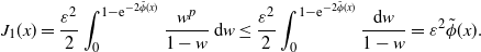 \begin{equation} J_1(x) = \frac{\varepsilon^2}{2}\int_0^{1-\mathrm{e}^{-2\tilde{\phi}(x)}}\frac{w^p}{1-w}\,{\mathrm{d}} w \leq \frac{\varepsilon^2}{2}\int_0^{1-\mathrm{e}^{-2\tilde{\phi}(x)}}\frac{{\mathrm{d}} w}{1-w} = \varepsilon^2\tilde{\phi}(x). \end{equation}
The second integral
 $J_2$
can be calculated explicitly, giving, if we use (15),
$J_2$
can be calculated explicitly, giving, if we use (15),
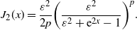 \begin{equation} J_2(x) = \frac{\varepsilon^2}{2p}\bigg(\frac{\varepsilon^2}{\varepsilon^2+\mathrm{e}^{2x}-1}\bigg)^p. \end{equation}
 \begin{equation} \int_0^\infty\int_0^\infty|R(x,y)|^p\,{\mathrm{d}} x\,{\mathrm{d}} y \leq 2^p\varepsilon^2\int_0^\infty\mathrm{e}^{-2px}\tilde{\phi}(x)\,{\mathrm{d}} x + \varepsilon^2\frac{2^p}{2p}\int_0^\infty\frac{(1-\mathrm{e}^{-2x})^p}{(\varepsilon^2+\mathrm{e}^{2x}-1)^p}\,{\mathrm{d}} x. \end{equation}
Denote the two integrals in (21) by
 $K_1$
and
$K_1$
and
 $K_2$
.
$K_2$
.
We deal with
 $K_1$
first and start with the following upper bound for
$K_1$
first and start with the following upper bound for
 $\tilde{\phi}$
:
$\tilde{\phi}$
:
 \[ \tilde{\phi}(x) = \frac{1}{2}\ln\bigg(\frac{\varepsilon^2+\mathrm{e}^{2x}-1}{\varepsilon^2}\bigg) = \frac{1}{2}\ln(\varepsilon^2+\mathrm{e}^{2x}-1) - \ln\varepsilon \leq \frac{1}{2}\ln(\mathrm{e}^{2x}) - \ln\varepsilon = x - \ln\varepsilon, \]
where we have used
 $\varepsilon \lt 1$
. This gives the estimate
$\varepsilon \lt 1$
. This gives the estimate
 \begin{equation} K_1 \leq \int_0^\infty\mathrm{e}^{-2px}(x-\ln\varepsilon)\,{\mathrm{d}} x \leq -\mbox{const.}\,\ln\varepsilon \end{equation}
for some positive constant. For
 $K_2$
, which can be explicitly calculated for
$K_2$
, which can be explicitly calculated for
 $p=1,2$
, we easily find
$p=1,2$
, we easily find
 \begin{equation} K_2 \leq \frac{1}{2}. \end{equation}
By (21)–(23), we end up with
 $||R||_{L^p(G)} \leq \mbox{const.}\,\varepsilon^2(-\ln\varepsilon)$
,
$||R||_{L^p(G)} \leq \mbox{const.}\,\varepsilon^2(-\ln\varepsilon)$
,
 $p=1,2$
, which concludes the proof.
$p=1,2$
, which concludes the proof.
4. Validation of the formal approximation
We start this section with the formulation of the ABP result mentioned in the introduction. Its proof is a direct consequence of [Reference Grandits12, Theorem 2.1] if we set
 $G=\mathbf{R}^+\times\mathbf{R}^+$
,
$G=\mathbf{R}^+\times\mathbf{R}^+$
,
 $\rho=k=1$
.
$\rho=k=1$
.
Theorem 1. Consider the inhomogeneous linear elliptic PDE
 \[ {\mathcal K}H\,:\!=\,a_1 H_x+a_2 H_y+\frac{1}{2}\Delta^{(\epsilon)} H+f=0 \]
on G, with
 $H(x,0)=H(0,y)=0$
,
$H(x,0)=H(0,y)=0$
,
 $x,y\geq0$
, and
$x,y\geq0$
, and
 $\lim_{x\to\infty,y\to\infty}H(x,y)=0$
. Moreover, we assume that the
$\lim_{x\to\infty,y\to\infty}H(x,y)=0$
. Moreover, we assume that the
 $a_i$
are Borel measurable and
$a_i$
are Borel measurable and
 $a_1+a_2 =1$
,
$a_1+a_2 =1$
,
 $0\leq a_i \leq 1$
for
$0\leq a_i \leq 1$
for
 $i=1,2$
, and
$i=1,2$
, and
 $f \in L^\infty(G) \cap L^1(G) \cap L^2(G)$
. Then the boundary value problem for H has a unique solution in
$f \in L^\infty(G) \cap L^1(G) \cap L^2(G)$
. Then the boundary value problem for H has a unique solution in
 $W^{2,2}_{{\mathrm{loc}}}(G) \cap C(G)$
that fulfills
$W^{2,2}_{{\mathrm{loc}}}(G) \cap C(G)$
that fulfills
 \[ ||H||_{L^\infty(G)} \leq \frac{C}{\varepsilon}\big(\sqrt{\varepsilon}(-\ln\varepsilon)||f||_{L^2(G)}+||f||_{L^1(G)}\big) \]
for some positive constant C that does not depend on
 $\varepsilon$
.
$\varepsilon$
.
The aim of the rest of this section is twofold. First (see Remark 5), we want to prove that the formal approximation
 $\tilde{V}$
provided in (17) is indeed a valid approximation of the value function V(x,y) in
$\tilde{V}$
provided in (17) is indeed a valid approximation of the value function V(x,y) in
 $\overline{G}$
. We can easily give a strategy that produces
$\overline{G}$
. We can easily give a strategy that produces
 $\tilde{V}(x,y)$
as the target functional, namely
$\tilde{V}(x,y)$
as the target functional, namely
 $u = \small{\bigg(\begin{array}{c} 1 \\ 1\end{array}\bigg)}$
. Indeed, we have
$u = \small{\bigg(\begin{array}{c} 1 \\ 1\end{array}\bigg)}$
. Indeed, we have
 \[ J\bigg(x,y,\bigg(\begin{array}{c} 1 \\ 1\end{array}\bigg)\bigg) = {\mathbb{P}}_{x,y}(\tau_X \wedge \tau_Y=\infty) = {\mathbb{P}}_{x}(\tau_X=\infty){\mathbb{P}}_{y}(\tau_Y=\infty),\]
where
 $\tau_X\,:\!=\,\inf\{t \geq 0 \mid x+t+B^{(1)}_t \leq 0\}$
and
$\tau_X\,:\!=\,\inf\{t \geq 0 \mid x+t+B^{(1)}_t \leq 0\}$
and
 $\tau_Y\,:\!=\,\inf\{t \geq 0 \mid y+t+\varepsilon B^{(2)}_t \leq 0\}$
. Unfortunately,
$\tau_Y\,:\!=\,\inf\{t \geq 0 \mid y+t+\varepsilon B^{(2)}_t \leq 0\}$
. Unfortunately,
 $u= \small\left(\begin{array}{c} 1 \\ 1\end{array}\right)$
is not admissible.
$u= \small\left(\begin{array}{c} 1 \\ 1\end{array}\right)$
is not admissible.
The second and main aim of this section (see Theorem 2) is to provide an admissible strategy that gives a target functional approximating the value function V(x,y) uniformly in
 $\overline{G}$
.
$\overline{G}$
.
We consider the strategy
 \begin{equation*} \hat{u}(x,y)\,:\!=\, \left(\begin{array}{c} \mathbf{1}_{II}(x,y) \\ \mathbf{1}_I(x,y) \end{array}\right),\end{equation*}
with
 \begin{equation} I \,:\!=\, \{(x,y) \in G \mid y \lt \phi(x), x \gt 0\}, \qquad II \,:\!=\, \{(x,y) \in G \mid y \geq \phi(x), x \gt 0\},\end{equation}
where
 $\phi(x)$
is the separation curve defined in (17). Now let H(x,y) be the solution of the boundary value problem
$\phi(x)$
is the separation curve defined in (17). Now let H(x,y) be the solution of the boundary value problem
 \begin{equation} \begin{aligned} & {\mathcal L}^L H+f \,:\!=\, \mathbf{1}_{II}H_x + \mathbf{1}_{I}H_y + \frac{1}{2}\Delta^{(\epsilon)} H + f = 0 \mbox{ on }G, \\ & H(x,0) = H(0,y) = 0, \qquad \lim_{x\to\infty,y\to\infty}H(x,y)= 0, \end{aligned}\end{equation}
with
 $f(x,y)=-R(x,y)$
, and R as defined in Lemma 1. By Theorem 1, this solution is unique and an element of
$f(x,y)=-R(x,y)$
, and R as defined in Lemma 1. By Theorem 1, this solution is unique and an element of
 $W^{2,2}_{\mathrm{loc}}(G)$
. Moreover,
$W^{2,2}_{\mathrm{loc}}(G)$
. Moreover,
 \begin{equation} ||H||_{L^\infty(G)} \leq C(-\varepsilon \ln\varepsilon)\end{equation}
for some positive constant C, not depending on
 $\varepsilon$
. Consider now
$\varepsilon$
. Consider now
 $\hat{V}(x,y)\,:\!=\,\tilde{V}(x,y)-H(x,y)$
. Since, by construction,
$\hat{V}(x,y)\,:\!=\,\tilde{V}(x,y)-H(x,y)$
. Since, by construction,
 $\tilde{V}$
solves
$\tilde{V}$
solves
 ${\mathcal L}^L \tilde{V}+f=0$
,
${\mathcal L}^L \tilde{V}+f=0$
,
 $\hat{V}$
is the unique solution of
$\hat{V}$
is the unique solution of
 \begin{equation} {\mathcal L}^L \hat{V}=0\mbox{ on }G, \qquad \hat{V}(x,0)=\hat{V}(0,y)=0, \qquad \lim_{x\to \infty,y\to \infty}\hat{V}(x,y)= 1.\end{equation}
The next lemma shows that
 $\hat{V}(x,y)$
can be interpreted as the survival probability of
$\hat{V}(x,y)$
can be interpreted as the survival probability of
 $X_t$
and
$X_t$
and
 $Y_t$
if we use the admissible strategy
$Y_t$
if we use the admissible strategy
 $\hat{u}$
.
$\hat{u}$
.
Lemma 2.
If we denote the state process using the strategy
 $\hat{u}$
as
$\hat{u}$
as
 $\hat{Z}_t=(\hat{X}_t,\hat{Y}_t)=Z^{\hat{u}}_t$
and the corresponding exit time for G by
$\hat{Z}_t=(\hat{X}_t,\hat{Y}_t)=Z^{\hat{u}}_t$
and the corresponding exit time for G by
 $\hat{\tau}$
, we have
$\hat{\tau}$
, we have
 \[ \hat{V}(x,y) = \mathbb{P}_{x,y}(\hat{Z}_t \in G \ for\ all\ t \in \mathbf{R}_0^+) = \mathbb{P}_{x,y}(\hat{\tau} = \infty). \]
Proof. Let
 $\hat{\tau}_n \,:\!=\, \inf\{t \gt 0 \mid \hat{Z}_t \notin (1/n,n)\times(1/n,n)\}$
for n large enough that
$\hat{\tau}_n \,:\!=\, \inf\{t \gt 0 \mid \hat{Z}_t \notin (1/n,n)\times(1/n,n)\}$
for n large enough that
 $(x,y) \in (1/n,n)\times (1/n,n)$
. The Itô–Krylov formula (see, e.g., [Reference Krylov16, Section 2.10, Theorem 1] and Remark 4 here) gives
$(x,y) \in (1/n,n)\times (1/n,n)$
. The Itô–Krylov formula (see, e.g., [Reference Krylov16, Section 2.10, Theorem 1] and Remark 4 here) gives
 \begin{equation} \hat{V}(\hat{Z}_{t\wedge\hat{\tau}_n}) = \hat{V}(x,y) + \int_0^{t\wedge\hat{\tau}_n}\nabla\hat{V}(\hat{Z}_s) \mathop{\mathrm{diag}}(1,\varepsilon)\,{\mathrm{d}}\overline{B}_s + \int_0^{t\wedge\hat{\tau}_n}{\mathcal L}^L\hat{V}(\hat{Z}_s)\,{\mathrm{d}} s, \end{equation}
where
 $\overline{B}_t$
denotes
$\overline{B}_t$
denotes
 $\big(B^{(1)}_t,B^{(2)}_t\big)$
.
$\big(B^{(1)}_t,B^{(2)}_t\big)$
.
We have, almost surely (a.s.),
 $\hat{\tau}_n \to \hat{\tau}$
for
$\hat{\tau}_n \to \hat{\tau}$
for
 $n\to \infty$
, and hence
$n\to \infty$
, and hence
 $\hat{\tau}_n\wedge t \to \hat{\tau}\wedge t$
. Now, since
$\hat{\tau}_n\wedge t \to \hat{\tau}\wedge t$
. Now, since
 $\hat{V}$
,
$\hat{V}$
,
 $\hat{Z}_t$
, and the stochastic integral are continuous, and the last integral in (28) vanishes by assumption,
$\hat{Z}_t$
, and the stochastic integral are continuous, and the last integral in (28) vanishes by assumption,
 \begin{equation*} \hat{V}(\hat{Z}_{t\wedge\hat{\tau}}) = \hat{V}(x,y) + \int_0^{t\wedge\hat{\tau}}\nabla\hat{V}(\hat{Z}_s)\mathop{\mathrm{diag}}(1,\varepsilon)\,{\mathrm{d}}\overline{B}_s. \end{equation*}
Hence,
 $\hat{V}(\hat{Z}_{t\wedge\hat{\tau}})$
is a bounded local martingale, and hence a true martingale, even uniformly integrable. Therefore,
$\hat{V}(\hat{Z}_{t\wedge\hat{\tau}})$
is a bounded local martingale, and hence a true martingale, even uniformly integrable. Therefore,
 \begin{equation} \mathbb{E}_{x,y}[\hat{V}(\hat{Z}_{t\wedge\hat{\tau}})] = \hat{V}(x,y). \end{equation}
We can easily check, by Itô’s lemma (see also [Reference Grandits11, Proposition 3.1]), that
 $-\exp\{-2\hat{X}_{t\wedge\hat{\tau}}\}$
is a local supermartingale, bounded above and below. Therefore, this process is a true supermartingale, and hence
$-\exp\{-2\hat{X}_{t\wedge\hat{\tau}}\}$
is a local supermartingale, bounded above and below. Therefore, this process is a true supermartingale, and hence
 $\lim_{t \to \infty}-\exp\{-2\hat{X}_{t\wedge\hat{\tau}}\}$
exists a.s., and
$\lim_{t \to \infty}-\exp\{-2\hat{X}_{t\wedge\hat{\tau}}\}$
exists a.s., and
 $\lim_{t \to \infty}\hat{X}_{t\wedge\hat{\tau}}$
exists a.s. as well. Clearly, on the set
$\lim_{t \to \infty}\hat{X}_{t\wedge\hat{\tau}}$
exists a.s. as well. Clearly, on the set
 $\{\hat{\tau}=\infty\}$
this limit cannot be finite, and we get
$\{\hat{\tau}=\infty\}$
this limit cannot be finite, and we get
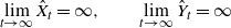 \begin{equation} \lim_{t \to \infty}\hat{X}_t=\infty, \qquad \lim_{t \to \infty}\hat{Y}_t=\infty \end{equation}
on
 $\{\hat{\tau}=\infty\}$
, since the same considerations hold for the process
$\{\hat{\tau}=\infty\}$
, since the same considerations hold for the process
 $\hat{Y}_t$
as well. All together,
$\hat{Y}_t$
as well. All together,
 $\hat{V}_{/\partial G}=0$
, the third equation of (27), and (30) give, after
$\hat{V}_{/\partial G}=0$
, the third equation of (27), and (30) give, after
 $t\to \infty$
in (29),
$t\to \infty$
in (29),
 \[ \mathbb{E}_{x,y}[\hat{V}(\hat{Z}_{\hat{\tau}})] = \mathbb{P}_{x,y}(\hat{\tau}=\infty)=\hat{V}(x,y), \]
which completes the proof.
Remark 4. Let us briefly comment on the usage of the generalized Itô formula, usually called the Itô–Krylov formula, in the previous proof. As noted, we have applied [Reference Krylov16, Section 2.10, Theorem 1]. There, the author uses the space
 $\bar{W}^2(D)$
(with
$\bar{W}^2(D)$
(with
 $D=(1/n,n)^2$
in our application). But this is nothing other than the usual Sobolev space
$D=(1/n,n)^2$
in our application). But this is nothing other than the usual Sobolev space
 $W^{2,2}(D)$
. Indeed, the (a priori) stronger norm, say
$W^{2,2}(D)$
. Indeed, the (a priori) stronger norm, say
 $|||\cdot|||_1$
, used for the completion process to come from
$|||\cdot|||_1$
, used for the completion process to come from
 $C^2(\overline{D})$
to
$C^2(\overline{D})$
to
 $\bar{W}^2(D)$
[Reference Krylov16, pp. 46--49] is equivalent to the usual Sobolev norm, say
$\bar{W}^2(D)$
[Reference Krylov16, pp. 46--49] is equivalent to the usual Sobolev norm, say
 $||\cdot||_{W^{2,2}(D)}$
, used for the completion process to come from
$||\cdot||_{W^{2,2}(D)}$
, used for the completion process to come from
 $C^2(\overline{D})$
to
$C^2(\overline{D})$
to
 $W^{2,2}(D)$
. The reason is that we can estimate the additional term in
$W^{2,2}(D)$
. The reason is that we can estimate the additional term in
 $|||\hat{V}|||_1$
, namely
$|||\hat{V}|||_1$
, namely
 $||\hat{V}_x||_{L^4(D)}+||\hat{V}_y||_{L^4(D)}$
, by
$||\hat{V}_x||_{L^4(D)}+||\hat{V}_y||_{L^4(D)}$
, by
 $C\,||\hat{V}||_{W^{2,2}(D)}$
for some positive constant C, since
$C\,||\hat{V}||_{W^{2,2}(D)}$
for some positive constant C, since
 $W^{2,2}$
is continuously embedded in
$W^{2,2}$
is continuously embedded in
 $W^{1,4}$
[Reference Adams and Fournier1, Theorem 4.12, I.B] (our domain D obviously fulfills the cone condition assumed there).
$W^{1,4}$
[Reference Adams and Fournier1, Theorem 4.12, I.B] (our domain D obviously fulfills the cone condition assumed there).
Our final theorem asserts that the strategy
 $\hat{u}$
indeed leads to a uniform approximation of the value function of the problem.
$\hat{u}$
indeed leads to a uniform approximation of the value function of the problem.
Theorem 2.
The target functional that we get by using the strategy
 $\hat{u}=\small\left(\begin{array}{c}\mathbf{1}_{II} \\ \mathbf{1}_{I}\end{array}\right)$
with the sets I and II defined in (24), i.e.
$\hat{u}=\small\left(\begin{array}{c}\mathbf{1}_{II} \\ \mathbf{1}_{I}\end{array}\right)$
with the sets I and II defined in (24), i.e.
 $\hat{V}(x,y)= \mathbb{P}_{x,y}(\tau^{\hat{u}}=\infty)$
, is a uniform approximation of the value function V(x,y) for the problem (1)–(3), with
$\hat{V}(x,y)= \mathbb{P}_{x,y}(\tau^{\hat{u}}=\infty)$
, is a uniform approximation of the value function V(x,y) for the problem (1)–(3), with
 $||V-\hat{V}||_{L^\infty(G)} \leq C(-\varepsilon\ln\varepsilon)$
for some positive,
$||V-\hat{V}||_{L^\infty(G)} \leq C(-\varepsilon\ln\varepsilon)$
for some positive,
 $\varepsilon$
-independent constant C.
$\varepsilon$
-independent constant C.
Proof. Obviously, by Lemma 2 we have the ordering
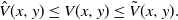 \begin{equation} \hat{V}(x,y) \leq V(x,y) \leq \tilde{V}(x,y). \end{equation}
Indeed,
 $\hat{V}$
is the target functional of one special admissible strategy, whereas V is the supremum over all admissible strategies of the target functional. Moreover, the drift of the strategy corresponding to
$\hat{V}$
is the target functional of one special admissible strategy, whereas V is the supremum over all admissible strategies of the target functional. Moreover, the drift of the strategy corresponding to
 $\tilde{V}$
, namely
$\tilde{V}$
, namely
 $u = \small\left(\begin{array}{c} 1 \\ 1\end{array}\right)$
, strictly dominates all admissible strategies. Since
$u = \small\left(\begin{array}{c} 1 \\ 1\end{array}\right)$
, strictly dominates all admissible strategies. Since
 $\hat{V}(x,y)=\tilde{V}(x,y)-H(x,y)$
with H as defined in (25), we see that
$\hat{V}(x,y)=\tilde{V}(x,y)-H(x,y)$
with H as defined in (25), we see that
 $0 \leq V(x,y)-\hat{V}(x,y) \leq H(x,y)$
holds. The theorem now follows by (26).
$0 \leq V(x,y)-\hat{V}(x,y) \leq H(x,y)$
holds. The theorem now follows by (26).
Remark 5. We also have
 $-H(x,y) \leq V(x,y) -\tilde{V}(x,y) \leq 0$
, which shows that
$-H(x,y) \leq V(x,y) -\tilde{V}(x,y) \leq 0$
, which shows that
 $||\tilde{V}-V||_{L^\infty(G)} \leq C(-\varepsilon\ln\varepsilon)$
for some positive,
$||\tilde{V}-V||_{L^\infty(G)} \leq C(-\varepsilon\ln\varepsilon)$
for some positive,
 $\varepsilon$
-independent constant C.
$\varepsilon$
-independent constant C.
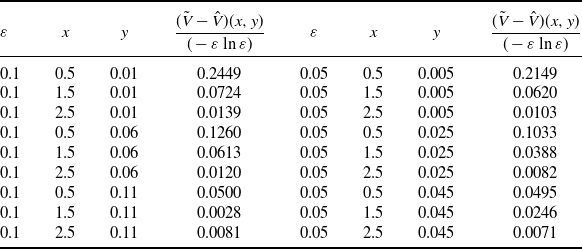
Remark 6. Theorem 2 gives the upper bound
 $C(-\varepsilon\ln\varepsilon)$
for the difference of the value function and the target functional produced by our strategy
$C(-\varepsilon\ln\varepsilon)$
for the difference of the value function and the target functional produced by our strategy
 $\hat{u}$
, i.e. for
$\hat{u}$
, i.e. for
 $||V-\hat{V}||_{L^\infty(G)}$
. We noted there that the constant C does not depend on
$||V-\hat{V}||_{L^\infty(G)}$
. We noted there that the constant C does not depend on
 $\varepsilon$
. For practical reasons it would, of course, be interesting to have an idea about the actual size of this constant. From (31), it is clear that
$\varepsilon$
. For practical reasons it would, of course, be interesting to have an idea about the actual size of this constant. From (31), it is clear that
 ${||\tilde{V}-\hat{V}||_{L^\infty(G)}}/{(-\varepsilon\ln\varepsilon)}$
is an upper bound for this C. We performed a Monte Carlo simulation to get an estimate for
${||\tilde{V}-\hat{V}||_{L^\infty(G)}}/{(-\varepsilon\ln\varepsilon)}$
is an upper bound for this C. We performed a Monte Carlo simulation to get an estimate for
 $(\tilde{V}-\hat{V})(x,y)$
for nine different starting values (x,y) and two values of epsilon, with three of the points lying below the separation curve
$(\tilde{V}-\hat{V})(x,y)$
for nine different starting values (x,y) and two values of epsilon, with three of the points lying below the separation curve
 $\phi(x)$
and six above. We provide the results in Table 1. For each initial value we simulated 100 000 paths with a time step given by 1/80 000. It can be seen that the constant is reasonably small.
$\phi(x)$
and six above. We provide the results in Table 1. For each initial value we simulated 100 000 paths with a time step given by 1/80 000. It can be seen that the constant is reasonably small.
Table 1. Results of the Monte Carlo simulation.
5. Conclusion
As soon as we try to consider ruin problems in insurance for more than one company (say, for convenience, for two), the question of how the wealth processes of the two firms should interact arises. We believe that a very natural possibility is to allow payments between them. Now, the question is, what should be the goal of this interaction? Or, in mathematical terms, how should we choose the target functional of an optimization problem? We believe that choosing the maximization of the probability that both companies survive is a very natural possibility. We have considered this problem in our article for the case where one firm faces a small volatility, say
 $\varepsilon$
, in comparison to the other one, and constructed a strategy that gives a uniform approximation of the value function for small
$\varepsilon$
, in comparison to the other one, and constructed a strategy that gives a uniform approximation of the value function for small
 $\varepsilon$
.
$\varepsilon$
.
Of course, generalizations of our model are numerous. For example, we could consider Cramér–Lundberg wealth processes instead of diffusion processes, or more than two companies. We believe that these kinds of problems are interesting, but not easy to solve; they are left for future research.
Appendix
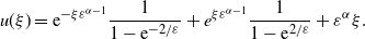
In this appendix we want to illustrate some concepts of singular perturbation theory by a simple one-dimensional example. We confine ourselves to first-order approximation. Consider the differential equation
 $\varepsilon^2 u^{\prime\prime}(x)-u(x)+x=0$
, with the boundary conditions
$\varepsilon^2 u^{\prime\prime}(x)-u(x)+x=0$
, with the boundary conditions
 $u(0)=u(1)=1$
. This problem has the explicit solution
$u(0)=u(1)=1$
. This problem has the explicit solution
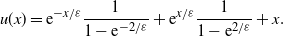 \begin{equation*} u(x) = \mathrm{e}^{-x/\varepsilon}\frac{1}{1-\mathrm{e}^{-2/\varepsilon}} + \mathrm{e}^{x/\varepsilon}\frac{1}{1-\mathrm{e}^{2/\varepsilon}} + x.\end{equation*}
Typically, ODEs with a small parameter in front of the highest-order derivative do not posses solutions with a regular approximation, i.e. a function not depending on
 $\varepsilon$
approximating the solution uniformly. Rather, they have a so-called boundary layer, a region near the boundary where the solution has a large gradient (depending on
$\varepsilon$
approximating the solution uniformly. Rather, they have a so-called boundary layer, a region near the boundary where the solution has a large gradient (depending on
 $\varepsilon$
). The goal is now to find an approximation of the solution in this region. This is done by using a kind of ‘mathematical magnifying glass’, i.e. we consider the function depending on a different independent variable, say
$\varepsilon$
). The goal is now to find an approximation of the solution in this region. This is done by using a kind of ‘mathematical magnifying glass’, i.e. we consider the function depending on a different independent variable, say
 $\xi$
, and take the limit
$\xi$
, and take the limit
 $\varepsilon \to 0$
. The result is called a local limit of u with respect to
$\varepsilon \to 0$
. The result is called a local limit of u with respect to
 $\xi$
, i.e.
$\xi$
, i.e.
 $\tilde{u}(\xi)=\lim_{\varepsilon \to 0}u(\xi(x))$
. Now, if we have two different local variables, say
$\tilde{u}(\xi)=\lim_{\varepsilon \to 0}u(\xi(x))$
. Now, if we have two different local variables, say
 $\xi_1$
and
$\xi_1$
and
 $\xi_2$
, we say the local limit with respect to
$\xi_2$
, we say the local limit with respect to
 $\xi_2$
is contained in that of
$\xi_2$
is contained in that of
 $\xi_1$
if, with
$\xi_1$
if, with
 $\tilde{u}(\xi_1)=\lim_{\varepsilon \to 0}u(\xi_1(x))$
and
$\tilde{u}(\xi_1)=\lim_{\varepsilon \to 0}u(\xi_1(x))$
and
 $\hat{u}(\xi_2)=\lim_{\varepsilon \to 0}u(\xi_2(x))$
,
$\hat{u}(\xi_2)=\lim_{\varepsilon \to 0}u(\xi_2(x))$
,
 $\hat{u}(\xi_2)=\lim_{\varepsilon \to 0}\tilde{u}(\xi_1(\xi_2))$
. Finally, a local limit which is not contained in any other is called a significant local limit, and provides the best information about the solution near the critical boundary. Moreover, the corresponding independent variable is called a boundary layer variable.
$\hat{u}(\xi_2)=\lim_{\varepsilon \to 0}\tilde{u}(\xi_1(\xi_2))$
. Finally, a local limit which is not contained in any other is called a significant local limit, and provides the best information about the solution near the critical boundary. Moreover, the corresponding independent variable is called a boundary layer variable.

Figure 2. Plots of u(x),
 $u^*(x)$
, and
$u^*(x)$
, and
 $\bar{u}(x)$
for
$\bar{u}(x)$
for
 $\varepsilon=0.02$
.
$\varepsilon=0.02$
.
Now, back to our example. If we consider the transformation
 $\xi={x}/{\varepsilon^\alpha}$
with
$\xi={x}/{\varepsilon^\alpha}$
with
 $\alpha \gt 0$
, we find that
$\alpha \gt 0$
, we find that
 \begin{equation*} u(\xi) = \mathrm{e}^{-\xi\varepsilon^{\alpha-1}}\frac{1}{1-\mathrm{e}^{-2/\varepsilon}} + e^{\xi\varepsilon^{\alpha-1}}\frac{1}{1-\mathrm{e}^{2/\varepsilon}} + \varepsilon^\alpha\xi.\end{equation*}
For
 $\alpha=1$
, we get the local limit
$\alpha=1$
, we get the local limit
 $u^*(\xi)=e^{-\xi}$
; for
$u^*(\xi)=e^{-\xi}$
; for
 $\alpha \gt 1$
,
$\alpha \gt 1$
,
 $u^{(\alpha)}\equiv 1$
; and for
$u^{(\alpha)}\equiv 1$
; and for
 $\alpha \lt 1$
,
$\alpha \lt 1$
,
 $u^{(\alpha)}\equiv 0$
. Clearly, the latter two local limits are contained in
$u^{(\alpha)}\equiv 0$
. Clearly, the latter two local limits are contained in
 $u^*(\xi)$
(this is most easily seen by letting
$u^*(\xi)$
(this is most easily seen by letting
 $\xi\to 0$
, resp.
$\xi\to 0$
, resp.
 $\xi \to \infty$
, in
$\xi \to \infty$
, in
 $u^*(\xi)$
). Hence,
$u^*(\xi)$
). Hence,
 $u^*(\xi)$
is a significant local limit, and
$u^*(\xi)$
is a significant local limit, and
 $\xi=x/\varepsilon$
the corresponding boundary layer variable.
$\xi=x/\varepsilon$
the corresponding boundary layer variable.
Since the solution function is not always known, the problem is to find a good approximation in the critical region. This is done by the so-called ‘heuristic principle’, which we explain now.
As before, we express the given differential operator, say
 ${\mathcal L}^x$
, with respect to different independent variables, say
${\mathcal L}^x$
, with respect to different independent variables, say
 $\xi$
, and take
$\xi$
, and take
 $\varepsilon$
to zero. We get the degeneration
$\varepsilon$
to zero. We get the degeneration
 ${\mathcal L}^{\xi,0}$
.
${\mathcal L}^{\xi,0}$
.
If we also get the operator
 ${\mathcal L}^{\xi_2,0}$
from first going to
${\mathcal L}^{\xi_2,0}$
from first going to
 ${\mathcal L}^{\xi_1,0}$
and then to
${\mathcal L}^{\xi_1,0}$
and then to
 ${\mathcal L}^{\xi_2,0}$
, we say that
${\mathcal L}^{\xi_2,0}$
, we say that
 ${\mathcal L}^{\xi_2,0}$
is contained in
${\mathcal L}^{\xi_2,0}$
is contained in
 ${\mathcal L}^{\xi_1,0}$
. A significant degeneration is one that is not contained in any other degeneration.
${\mathcal L}^{\xi_1,0}$
. A significant degeneration is one that is not contained in any other degeneration.
Finally, the heuristic principle says that significant degenerations correspond to boundary layer variables [Reference Meyer and Parter21, Chapter I.1.4, p. 10]. In our example, we find that
 \begin{equation*} \varepsilon^{2-2\alpha}\frac{{\mathrm{d}}^2u}{{\mathrm{d}}\xi^2}-u(\xi)+\xi\varepsilon^\alpha=0.\end{equation*}
For
 $\alpha=1$
, this gives
$\alpha=1$
, this gives
 \begin{equation} \frac{{\mathrm{d}}^2u}{{\mathrm{d}}\xi^2}-u(\xi)=0.\end{equation}
For
 $\alpha \gt 1$
we get, after renorming,
$\alpha \gt 1$
we get, after renorming,
 \begin{equation*} \frac{{\mathrm{d}}^2u}{{\mathrm{d}}\xi^2}=0,\end{equation*}
and for
 $\alpha \lt 1$
we get
$\alpha \lt 1$
we get
 $u(\xi)=0$
. Obviously, (32) is the significant degeneration.
$u(\xi)=0$
. Obviously, (32) is the significant degeneration.
Away from the critical boundary, the solution, say
 $\bar{u}$
, of the so-called reduced equation (just set
$\bar{u}$
, of the so-called reduced equation (just set
 $\varepsilon=0$
in the original ODE) typically gives a valid approximation. In our case we have
$\varepsilon=0$
in the original ODE) typically gives a valid approximation. In our case we have
 $\bar{u}=x$
as a solution of
$\bar{u}=x$
as a solution of
 $-u+x=0$
. Plots of the solution function u(x) (solid line) and the two approximations
$-u+x=0$
. Plots of the solution function u(x) (solid line) and the two approximations
 $u^*(x)$
(dashed) and
$u^*(x)$
(dashed) and
 $\bar{u}(x)$
(dotted) can be found in Figure 2.
$\bar{u}(x)$
(dotted) can be found in Figure 2.
Acknowledgements
I thank two anonymous reviewers for carefully reading the paper, and for suggestions to improve it. I would also like to thank Micheal Leidl for providing the numerics described in Remark 6.
Funding information
Support from the Austrian Science Foundation (Fonds zur Förderung der wissenschaftlichen Forschung), Project no. P26487, is gratefully acknowledged.
Competing interests
There were no competing interests to declare which arose during the preparation or publication process of this article.


 Open access