Socio-economic deprivation, as measured by the Jarman under-privileged area (UPA) score (Reference JarmanJarman, 1983) and other measures, is associated with a high prevalence of disease, including severe mental illness (Reference Thornicroft, Margolius and JonesThornicroft et al, 1992; Reference AchesonAcheson, 1998). In the general population the prevalence of depression correlates with area deprivation (Reference Eachus, Williams and ChanEachus et al, 1996), individual characteristics such as unemployment (Reference Meltzer, Gill and PetticrewMeltzer et al, 1995) and employment grade (Stansfield & Marmot, 1992). However, consecutive consulting samples in primary care are potentially more useful to the clinician, reflecting the effects on day-to-day practice. Only the early study of Shepherd et al (Reference Shepherd, Cooper and Brown1966) has taken such a primary care perspective and none has evaluated the relative influence of locality v. individual deprivation, nor the influence of deprivation on outcome. An opportunity to do so arose in the context of the Hampshire Depression Project (HDP), a randomised controlled trial of an educational package on depression (Reference Thompson, Kinmonth and StevensThompson et al, 2000).
METHOD
Subjects
Fifty-five out of 224 (26%) practices in Hampshire, including 152 practitioners (69% of all partners), agreed to take part in a randomised controlled trial of an educational intervention. The practices were representative of Hampshire (see Table 1 in Reference Thompson, Kinmonth and StevensThompson et al, 2000 for details). In four separate phases, from November 1994 to March 1997, consecutive adult patients (16 years and over) attending routine surgeries were screened by researchers distributing questionnaires in the waiting room. In each phase, screening continued until 50 (where there was one practitioner taking part) or 30 (where there was more than one study doctor in the practice) valid questionnaires per practitioner had been obtained. Patients were excluded if they were too physically ill or unable to complete the questionnaire.
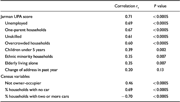
Table 1 Spearman's correlation coefficients for the Jarman under-privileged area (UPA) score, un-transformed constituent census variables, housing tenancy and car ownership with standardised practice probable case ratios
| Correlation r s | P value | |
|---|---|---|
| Jarman UPA score | 0.71 | <0.0005 |
| Unemployed | 0.69 | <0.0005 |
| One-parent households | 0.67 | <0.0005 |
| Unskilled | 0.61 | <0.0005 |
| Overcrowded households | 0.60 | <0.0005 |
| Children under 5 years | 0.39 | 0.002 |
| Ethnic minority households | 0.35 | 0.007 |
| Elderly living alone | 0.35 | 0.007 |
| Change of address in past year | 0.20 | 0.13 |
| Census variables | ||
| Not owner-occupier | 0.46 | <0.0005 |
| % households with no car | 0.69 | <0.0005 |
| % households with two or more cars | -0.70 | <0.0005 |
A total of 20 832 valid screening questionnaires were collected over the four screening phases. Duplicates were avoided by including only the first attendance of patients with an identical gender, date of birth and practice, and excluding forms where this was unavailable, leaving 18 414 patients (85.4% of the whole sample).
Measures of depression and employment
Two questionnaires were administered to each patient containing: (a) a brief explanation of the study, a request for demographic information and employment status in eight categories; (b) the Hospital Anxiety and Depression (HAD) scale (Reference Zigmond and SnaithZigmond & Snaith, 1983), which yields separate scores for symptoms of anxiety (A) and depression (D). Each scale has seven items, scores 0-3. There are no items related to biological symptoms of anxiety or depression, thus allowing exclusion of artificially high scores due to comorbidity with physical illness. The scale has been validated as a screening tool in general practice (Reference Wilkinson and BarczakWilkinson & Barczak, 1988) and has been shown to be sensitive to change (Reference HerrmanHerrman, 1997).
There are two levels of case definition for the D scale: ‘possible depression’ at ≥8 and ‘probable depression’ at ≥11. Both thresholds were used in this study. All patients with possible depression were sent another HAD by post 6 weeks and 6 months later. Patients who did not respond were sent another 2 weeks later. Questionnaires returned more than 12 weeks after the census date were excluded. At both of these times ‘remission’ was defined as a D score less than 8 and ‘improvement’ was defined as a score 50% or less than at the index consultation. For practice prevalence estimates, the higher threshold of ≥ 11 was used (probable depression), as it has a greater specificity against clinically diagnosed depression (Reference Upadhyaya and StanleyUpadhyaya & Stanley, 1993).
At each consultation, practitioners rated depression on a 4-point scale. Ratings of 2: ‘clinically significant depressive illness, mild’, and 3: ‘clinically significant depressive illness, moderate or severe’ indicated recognition of the depression.
Measures of deprivation
The UPA scores for each electoral ward, taken from the 1991 census, were used as the index of deprivation. Patients were allocated the deprivation scores for the practice (or branch surgery) where the index consultation took place, irrespective of their own address. The non-UPA statistics from the 1991 census (Office of Population Censuses and Surveys, 1993) for car ownership and housing tenure have also been included as they appear in other measures of deprivation (Reference Morris and CarstairsMorris & Carstairs, 1991).
Data analysis
For each practice, indirect standardisation was used to adjust for age (in 10-year age bands) and gender differences in practice samples. Standardised practice prevalence ratios of probable depression were calculated by dividing the number of observed by expected cases. The relation between crude and standardised practice case prevalence and UPA score was modelled using linear regression.
At the patient level, two analyses were carried out, one using ‘probable cases’ examined prevalence and the other using ‘possible cases’ (including all probable cases) examined outcome. Multiple logistic regression was used to estimate odds ratios (ORs) for risk of probable depression. A series of models were constructed with probable depression as the dependent variable. Individual covariates of gender, age and employment status were added to the model. Odds ratios for the UPA are presented for an increase of 10 points. The final model included all possible two-way interactions with backward stepwise selection to remove non-significant terms at P < 0.05. Multiple logistic regression was used in the ‘possible cases’ to identify variables predicting ‘remission’ and ‘improvement’. The following covariates were entered: age, gender and employment status, recognition of depression by the practitioner, depression and anxiety scores at index consultation, practice UPA score. The analyses were controlled for fund-holding and mental health resources. Interaction terms were not explored. Backward stepwise selection was used to remove non-significant variables at P < 0.05. Statistical procedures were performed in SPSS 6.1.2 for Windows.
RESULTS
Patients
Records of questionnaire completion were made in the second and fourth phases of screening and the average response rate was 89%, i.e. 11% of eligible patients were unable or unwilling to complete the screening instruments. There were no significant associations between practice UPA score and response rate (Spearman's correlation coefficient, 0.05, P=0.74 and ‒0.04, P=0.75).
Of the patients, 12 168 (66.1%) were female and 6246 (33.9%) were male. The youngest patient was 16 and there were 194 aged between 85 and 94 years. The number of possible cases was 3668 (19.9%) patients and of these 2299 (62.7%) returned a HAD at 6 weeks and 1956 (53.3%) at 6 months. Respondents at 6 weeks did not differ significantly from non-responders in depression or anxiety scores at the index consultation (Mann-Whitney U-test, Z=-1.81, P=0.07 and Z=-0.84, P=0.40) or UPA score (Mann-Whitney U-test, Z=-0.298, P=0.77). Neither did they differ in the eventual HAD scores at 6 months' follow-up (Mann-Whitney U-test, Z=-0.475, P=0.64 and Z=-0.841, P=0.40). However, women were more likely to return questionnaires at 6 week follow-up (χ2=8.62, d.f.=1, P=0.003), and the response rate was positively associated with age at both assessments. At 6 months, patients from high UPA practice areas were less likely to return the questionnaire (Mann-Whitney U-test, Z=-0.287, P=0.004), possibly confounded by greater geographical mobility.
Prevalence of depressive symptoms and deprivation scores of the practice location
The mean practice prevalence of probable depression was 7.2% (s.d. 2.6%), ranging from 2.4% to 13.7% (χ2=169.8, d.f.=57, P<0.0001). The regression of crude practice prevalence rates (n=58 surgery addresses) against UPA score gives β=0.10 (95% CI 0.07-0.13) and r 2=45.3%. The regression of standardised probable case ratios against UPA gives β=1.43 (%) (95% CI 1.03-1.82), r 2=48.3% (Fig. 1). Analysis excluding the two practices with extreme UPA scores reduced the attributable variance only slightly to r 2=45.2%.
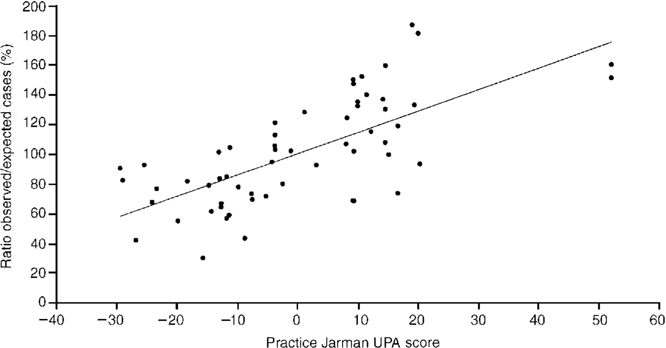
Fig. 1 Age- and gender-adjusted prevalence of high depression scores on the Hospital Anxiety and Depression (HAD) scale (HAD-D ≥ 11) in 58 practice sites showing association with the Jarman under-privileged area (UPA) score of the electoral ward in which the practice is located.
Each of the eight variables of the UPA score together with car ownership and housing tenancy was examined separately for its correlation with the standardised probable case ratios (Table 1). Geographical mobility (change of address in the past year) was the only variable that did not correlate significantly. The percentage of households with two or more cars was the most highly correlated single variable (r s=-0.70) with unemployment close behind (0.69).
Figure 2 shows frequency curves for practices falling above and below the median UPA score. The correlation of probable cases with deprivation appears to be due to an increase across the range of mild to moderate severity (D score 6-17) rather than to a small excess of severe cases or to a right shift in the whole population (Reference Anderson, Huppert and RoseAnderson et al, 1993).
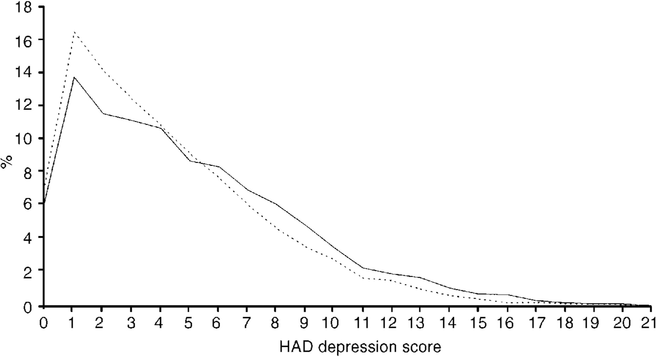
Fig. 2 Hospital Anxiety and Depression (HAD) D scores for patients attending practices in the upper and lower quartiles ranked by Jarman under-privileged area (UPA) score; ----, least-deprived quartile; [UNK], most-deprived quartile
Associations between individual characteristics and depression
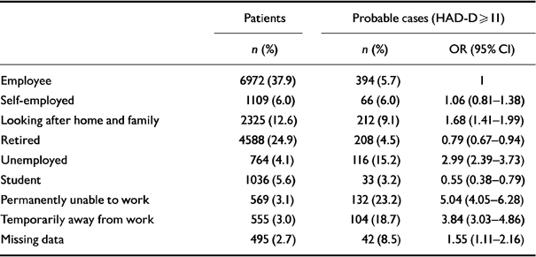
All age groups from 25 years to 54 years had significantly raised ORs for depression prevalence compared to the age group 16-24 years, and the ORs fell below 1.0 (but not significantly) for all groups over 65 years. Exactly 7.1% of both females and males were cases and there was therefore no association with gender. The unemployed, temporarily away from work or permanently unable to work, and those looking after home and family, were significantly more likely to be depressed than those in employment (Table 2). The retired and student groups were at lower risk than employees.
Table 2 Odds ratios for risk of probable caseness by individual employment status
| Patients | Probable cases (HAD-D ≥ 11) | ||
|---|---|---|---|
| n (%) | n (%) | OR (95% CI) | |
| Employee | 6972 (37.9) | 394 (5.7) | 1 |
| Self-employed | 1109 (6.0) | 66 (6.0) | 1.06 (0.81-1.38) |
| Looking after home and family | 2325 (12.6) | 212 (9.1) | 1.68 (1.41-1.99) |
| Retired | 4588 (24.9) | 208 (4.5) | 0.79 (0.67-0.94) |
| Unemployed | 764 (4.1) | 116 (15.2) | 2.99 (2.39-3.73) |
| Student | 1036 (5.6) | 33 (3.2) | 0.55 (0.38-0.79) |
| Permanently unable to work | 569 (3.1) | 132 (23.2) | 5.04 (4.05-6.28) |
| Temporarily away from work | 555 (3.0) | 104 (18.7) | 3.84 (3.03-4.86) |
| Missing data | 495 (2.7) | 42 (8.5) | 1.55 (1.11-2.16) |
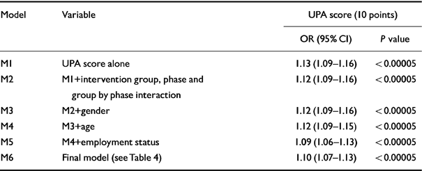
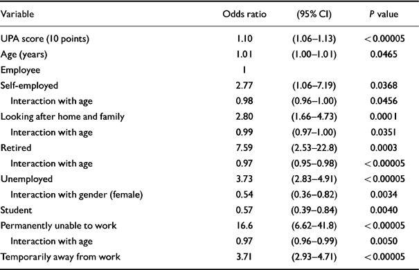
The relationship between the two main variables was further analysed to examine the effect of practice UPA score on the odds of an individual patient being a case. Here, the UPA score of the patient's practice becomes a variable belonging to the patient. Tables 3 and 4 show the effect of UPA score in these models. The important result is that individual patient variables account for some, but not all of the variance and the UPA score remained significant after adjusting for these effects. The odds of being a case increase by 1.10 (1.06 to 1.13) for every 10 UPA points, or 1.37 (1.24 to 1.52) for 34 UPA points (2 standard deviations).
Table 3 The effect of the Jarman under-privileged area (UPA) score on the odds of being a case, adjusted for the intervention of the randomised controlled trial from which the sample was derived, the phase at which the patient was screened, gender, age, and employment status (n=18 414)
| Model | Variable | UPA score (10 points) | |
|---|---|---|---|
| OR (95% CI) | P value | ||
| M1 | UPA score alone | 1.13 (1.09-1.16) | <0.00005 |
| M2 | M1+intervention group, phase and group by phase interaction | 1.12 (1.09-1.16) | <0.00005 |
| M3 | M2+gender | 1.12 (1.09-1.16) | <0.00005 |
| M4 | M3+age | 1.12 (1.09-1.15) | <0.00005 |
| M5 | M4+employment status | 1.09 (1.06-1.13) | <0.00005 |
| M6 | Final model (see Table 4) | 1.10 (1.07-1.13) | <0.00005 |
Table 4 Adjusted odds ratios (95% CI) for each significant variable in the final model
| Variable | Odds ratio | (95% CI) | P value |
|---|---|---|---|
| UPA score (10 points) | 1.10 | (1.06-1.13) | <0.00005 |
| Age (years) | 1.01 | (1.00-1.01) | 0.0465 |
| Employee | 1 | ||
| Self-employed | 2.77 | (1.06-7.19) | 0.0368 |
| Interaction with age | 0.98 | (0.96-1.00) | 0.0456 |
| Looking after home and family | 2.80 | (1.66-4.73) | 0.0001 |
| Interaction with age | 0.99 | (0.97-1.00) | 0.0351 |
| Retired | 7.59 | (2.53-22.8) | 0.0003 |
| Interaction with age | 0.97 | (0.95-0.98) | <0.00005 |
| Unemployed | 3.73 | (2.83-4.91) | <0.00005 |
| Interaction with gender (female) | 0.54 | (0.36-0.82) | 0.0034 |
| Student | 0.57 | (0.39-0.84) | 0.0040 |
| Permanently unable to work | 16.6 | (6.62-41.8) | <0.00005 |
| Interaction with age | 0.97 | (0.96-0.99) | 0.0050 |
| Temporarily away from work | 3.71 | (2.93-4.71) | <0.00005 |
Unemployed women were less likely to be depressed than unemployed men. The self-employed, those permanently unable to work or looking after home and family were less likely to be depressed if they were older. There were no significant interaction terms with UPA score and employment status, suggesting that the effects of unemployment were as important in residents of socio-economically deprived areas as in wealthier parts.
Predictors of outcome in possible depression
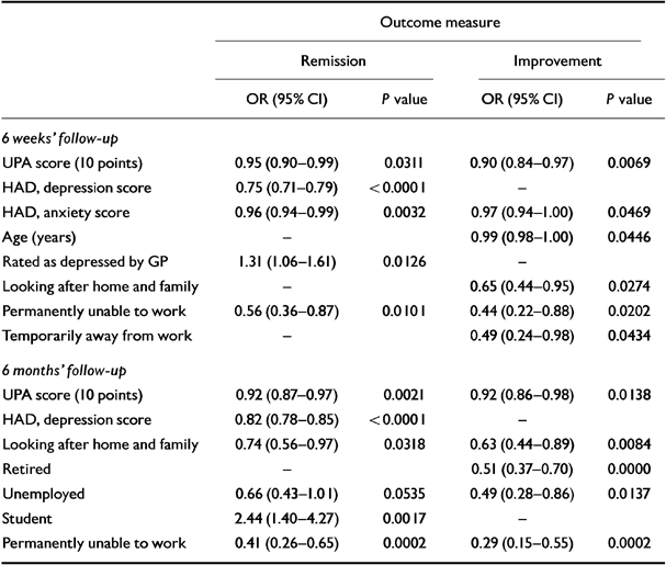
The variables that significantly predicted outcome in the logistic regression models are shown in Table 5. Higher UPA scores most strongly predicted poor outcome at both 6 weeks and 6 months, for both remission and improvement. Remission was predicted by a lower initial severity of depression and anxiety and being a student. Improvement was independent of initial severity of depression but adversely influenced by anxiety.
Table 5 Factors at baseline that significantly predicted 6-week and 6-month outcome in those with possible depression
| Outcome measure | ||||
|---|---|---|---|---|
| Remission | Improvement | |||
| OR (95% CI) | P value | OR (95% CI) | P value | |
| 6 weeks' follow-up | ||||
| UPA score (10 points) | 0.95 (0.90-0.99) | 0.0311 | 0.90 (0.84-0.97) | 0.0069 |
| HAD, depression score | 0.75 (0.71-0.79) | <0.0001 | - | |
| HAD, anxiety score | 0.96 (0.94-0.99) | 0.0032 | 0.97 (0.94-1.00) | 0.0469 |
| Age (years) | - | 0.99 (0.98-1.00) | 0.0446 | |
| Rated as depressed by GP | 1.31 (1.06-1.61) | 0.0126 | - | |
| Looking after home and family | - | 0.65 (0.44-0.95) | 0.0274 | |
| Permanently unable to work | 0.56 (0.36-0.87) | 0.0101 | 0.44 (0.22-0.88) | 0.0202 |
| Temporarily away from work | - | 0.49 (0.24-0.98) | 0.0434 | |
| 6 months' follow-up | ||||
| UPA score (10 points) | 0.92 (0.87-0.97) | 0.0021 | 0.92 (0.86-0.98) | 0.0138 |
| HAD, depression score | 0.82 (0.78-0.85) | <0.0001 | - | |
| Looking after home and family | 0.74 (0.56-0.97) | 0.0318 | 0.63 (0.44-0.89) | 0.0084 |
| Retired | - | 0.51 (0.37-0.70) | 0.0000 | |
| Unemployed | 0.66 (0.43-1.01) | 0.0535 | 0.49 (0.28-0.86) | 0.0137 |
| Student | 2.44 (1.40-4.27) | 0.0017 | - | |
| Permanently unable to work | 0.41 (0.26-0.65) | 0.0002 | 0.29 (0.15-0.55) | 0.0002 |
Recognition of depression by the GP predicted remission (but not improvement) at 6 weeks but not at 6 months. No differential effect was found for gender. Older patients were less likely to have improved at 6 weeks and the retired group at 6 months. Thus the most consistent predictors of outcome were the socio-economic variables of area deprivation and individual employment status.
DISCUSSION
These results support an influence of socio-economic deprivation on both the prevalence and persistence of depression among general practice attenders that is of practical consequence. The UPA score accounted for almost half the inter-practice variation in prevalence - an effect produced by an increase in mild to moderate cases (D score 6-17). Individual characteristics of unemployment and car ownership were of comparable strength but the UPA score remained the strongest predictor of depression and of outcome up to 6 months later.
The general practices were representative of Hampshire, being larger than those in England as a whole and generally more affluent than inner-city or northern areas. However, they were situated in areas with a wide range of deprivation scores. The study was carried out within 4-5 years of the 1991 census from which UPA scores were derived. The definition of depression was not dependent on the accuracy of general practitioners' diagnoses, thus avoiding potential bias.
Limitations of the study
It was logistically impossible to carry out a diagnostic interview of more than 18 000 patients. We have therefore studied the prevalence of self-reported depressive symptoms rather than of an operationally defined diagnosis. Nevertheless, in primary care studies screening for depressive symptoms rather than syndromes is an appropriate strategy, since sub-syndromal major depression has been shown to contribute significantly to the public health burden (Reference Hays, Wells and SherbourneHays et al, 1995; Reference Olfson, Broadhead and WeissmanOlfson et al, 1996). For this purpose, the choice of the HAD appears to have been appropriate despite its modest sensitivity and specificity for DSM-III (American Psychiatric Association, 1980) mood disorders.
The sample of practices was broadly representative but it was not randomly selected since it depended upon at least one practitioner in each practice agreeing to take part. No inferences can be made from this study about depressive symptoms in the community at large nor about patients seen at home. However, it is known that home visits account for only 10% of doctor-patient contacts (Reference McCormick, Charlton and FlemingMcCormick et al, 1995) apart from elderly patients, where they are more frequent (35% at 75-84 years and 65% over 85 years), so the study results may not hold true for the elderly infirm.
The rate of follow-up was lower than we had expected and was affected by age, gender and UPA score, but not HAD scores, on at least one time point. It seems unlikely that the association we found between HAD and UPA scores was critically influenced by non-response in the absence of an association between response rate and HAD score. However, we cannot rule out the possibility that this association was affected by non-responders.
The measure of area deprivation was not exact because some patients might have lived in an adjacent electoral ward, not in that of the practice. This would have introduced a conservative bias into the associations. The UPA score has been criticised on a number of counts (Reference Morris and CarstairsMorris & Carstairs, 1991) and some have suggested that complex indices are unnecessary because unemployment rates alone are an adequate measure of deprivation (Reference Payne, Coy and MilnerPayne et al, 1993). We found positive correlations between depression and most component variables of the index but the total score showed a higher correlation than any single variable, with only unemployment and car owner-ship approaching it. The precise choice of index is probably irrelevant since they are all highly correlated (Reference Morris and CarstairsMorris & Carstairs, 1991).
We did not measure causes of poverty other than unemployment at the individual level so we have insufficient data fully to separate out the effects of area and individual deprivation, but correcting for individual unemployment only slightly reduced the effect of UPA score. It seems, therefore, that there may be an effect of living in a deprived area which may have an influence over and above that of individual deprivation.
Interpretation of the findings
Given the strength of these correlations it would not be unreasonable to assume that they are a reflection of those in the general population, even though they were measured in primary care attenders. If so, the associations we have demonstrated may come about through two main routes (Stansfield et al, 1998) and our results do not allow us to distinguish between them. First (the social cause hypothesis), living in a deprived area may cause depression perhaps with material insecurity, loss of social cohesion or a non-economic predisposing factor, such as certain types of early life experience acting as intervening variables (Reference Power and HertzmanPower & Hertzman, 1997). That the environment may play a part is suggested by studies that have reported reductions in mental illness after improvement in the urban environment (Reference HalpernHalpern, 1995). Second, there may be social selection with depressed individuals moving into deprived areas - as occurs with some suffering from schizophrenia (Reference Sloggett and JoshiSloggett & Joshi, 1994). The relative influence of social cause and social selection may vary with the economic climate (Reference Hammarstrom and JanlertHammarstrom & Janlert, 1997).
This is the first time that area deprivation has been examined as a predictor of the persistence of depression in consulting patients. Support for these findings can, however, be found in studies of individual risk factors where chronic social difficulties, low household income and perceived financial strain have been associated with the maintenance of depression (Reference Brown and MoranBrown & Moran, 1997; Reference Ronalds, Creed and StoneRonalds et al, 1997; Reference Weich, Churchill and LewisWeich et al, 1997).
The difference in the distribution of D scores in practices in the top and bottom quartile of the deprivation score is the kind described by Anderson et al (Reference Anderson, Huppert and Rose1993) as showing the presence of “a subset of individuals [who are] particularly exposed or susceptible [to a postulated cause acting at an individual level]”. This distinguishes it from a cause acting on a population, all of whom are equally susceptible, which would produce a right shift in the entire distribution.
Implications of the results
In practical terms, our findings have two implications for health policy. First, the emphasis on enhancing provision to deprived areas is correct, as anticipated, but there is no threshold above which the effects of deprivation begin to become apparent. Thus, any model of deprivation payments that has a built-in threshold will disadvantage those areas just below it. Since deprivation accounts for such a large proportion of the depression workload this may have a measurable effect on the equity of primary mental health care provision. Second, strategies to reduce the public health burden of depression might usefully combine population-based and high-risk approaches: for example, strong national environmental and employment policies in combination with health care that acknowledges the adverse influence of living in a deprived area. While individuals may benefit from specific treatments for depression there is little evidence that even their most effective use, without other measures, could significantly reduce the public health burden of the condition.
Clinical Implications and Limitations
CLINICAL IMPLICATIONS
-
▪ In primary care attenders, socio-economic deprivation accounted for half the large inter-practice variation in the prevalence of depression and predicted the persistence of depression over 6 months.
-
▪ The effect of deprivation appears to be exerted through its influence on vulnerable individuals rather than the whole population.
-
▪ Efforts at reducing the public health burden of depression should include social strategies as well as medical care.
LIMITATIONS
-
▪ The practices taking part were representative of Hampshire practices in all measured respects, but were not randomly selected.
-
▪ Cases were defined by scores on the Hospital Anxiety and Depression scale, not operational diagnostic criteria.
-
▪ The results from 6-week and 6-month follow-ups were based on modest response rates.
ACKNOWLEDGEMENTS
The study was funded by grants from the Medical Research Council, the South and West Regional Research and Development Committee and the Southampton Community Health Service NHS Trust. We thank Professor Brain Jarman for providing the scores for Hampshire and Professor T. Kendrick for helpful comments on the manuscript.




eLetters
No eLetters have been published for this article.