Introduction

Determining whether recent anthropogenic changes in atmospheric composition (in particular, the "greenhouse gases") are contributing to recent climate variations is a significant problem. One cannot observe the response of the climate system to individual forcings, as the forcings are all varying simultaneously, and the natural variability of the climate may be larger than the response from any one forcing. The role of sea ice in climate change is even more difficult to measure, as the observational record of ice cover is relatively short. Global, coupled atmosphere-ocean-ice general circulation models (GCMs) are the most comprehensive tools available for investigating these climate problems, as they permit individual forcings to be prescribed, and the role of sea ice in climate change can be diagnosed. Here we present the changes in Arctic sea-ice cover from GCM simulations of the years 1870−2100.

The Arctic Oscillation (AO), the dominant mode exhibited by wintertime surface pressures and temperatures, has been shown to influence Arctic ice concentrations and ice motion (Reference Walsh, Chapman and ShyWalsh and others, 1996; personal communication from I. Rigor, 1998). Recent analysis by Reference DeserDeser (2000) shows the hemispheric AO pattern is a superposition of two separate teleconnections patterns, and the AO signal over the Arctic is indistinguishable from the North Atlantic Oscillation (NAO). In this paper we present analysis of the teleconnections in the Arctic from a coupled atmosphere-ocean-ice GCM.

Model and Experiments

The Parallel Climate Model version 1 (PCM1) comprises the U.S. National Center for Atmospheric Research (NCAR) Community Climate Model version 3 (CCM3) atmospheric GCM at 2.8° × 2.8° resolution and 18 vertical levels (Reference Kiehl, Hack, Bonan, Boville, Williamson and RaschKiehl and others, 1998), the Parallel Ocean Program (POP) global ocean GCM with an average horizontal resolution of 0.66° and 31 vertical levels (Reference Dukowicz and SmithDukowicz and Smith, 1994) and a dynamic-thermodynamic sea-ice model. The CCM3 atmospheric GCM includes the radiative effects of a series of greenhouse gases ― CO² _, O₃ , CH₄, NO_x, CFC-11, CFC-12 and H₂O ― and the direct reflective effect of sulfate aerosols. The sea-ice thermodynamics are based on the Reference SemtnerSemtner (1976) model, with one internal ice temperature and one snow-layer temperature. The sea-ice dynamics uses the elasticviscous-plastic (EVP) rheology of Hunke and Dukowicz (1997), and the ice model runs on a grid with 27 km spacing over each hemisphere’s polar region. The sea-ice mass is represented by a single mean thickness per gridcell, without an evolving thickness distribution. More complete descriptions of the Parallel Climate Model and its sea-ice component are given in Reference WashingtonWashington and others (2000) and Weatherly and Zhang (in press).

The PCM1 was used to simulate climatic conditions through the years 1870−2100, using specified greenhouse gases and sulfate aerosols (hereafter, "greenhouse gases and sulfate aerosols" are referred to as GHGSA), and in some experiments, specifying a variable solar flux. The climate simulations were initialized by integrating the model to an equilibrium climate state with constant GHGSA estimated for 1870.

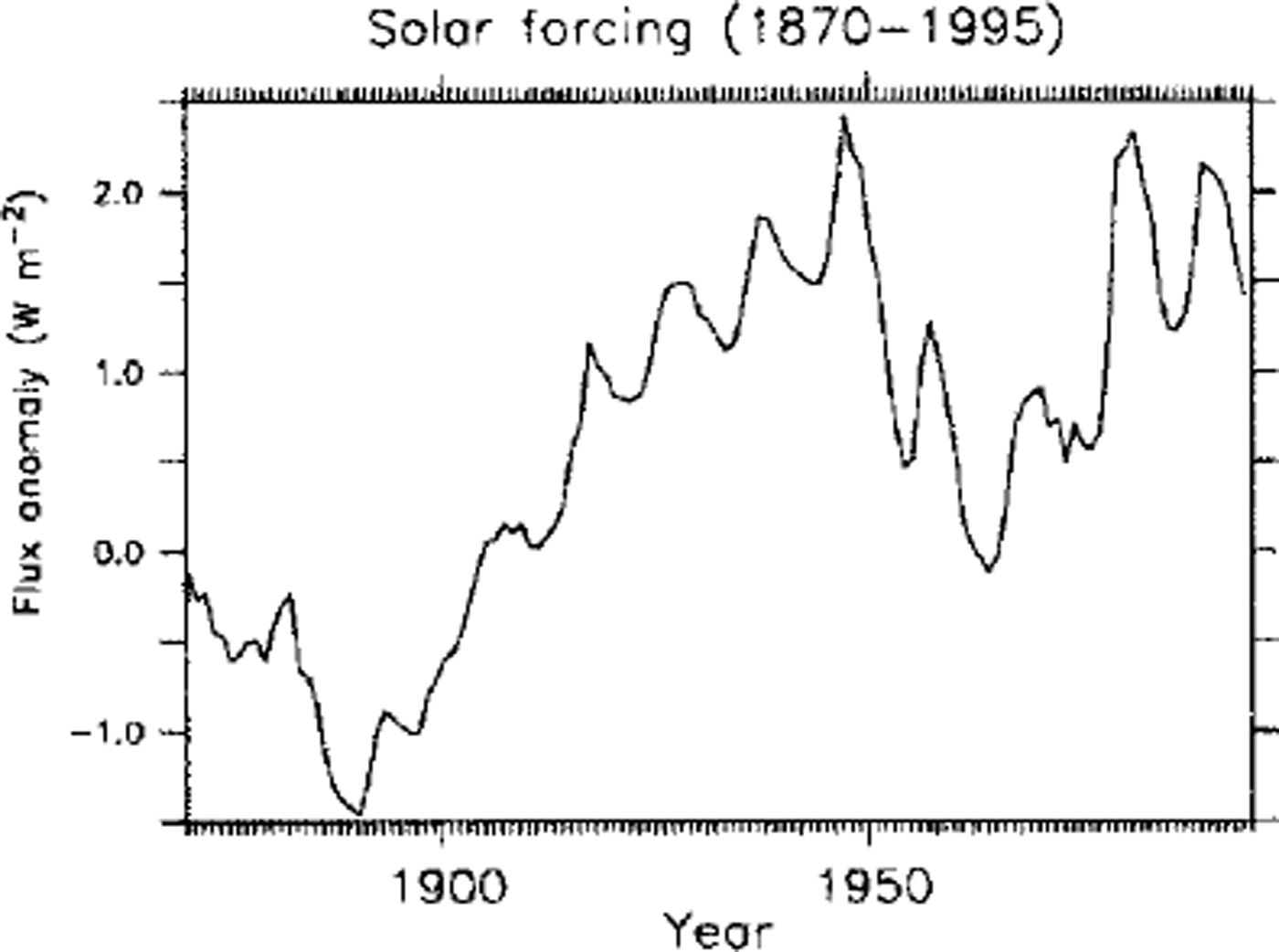
There were two types of simulations for 1870−1995, and two types of 1995−2100 simulations. The "Historical" simulations of the 1870−1995 climate used the GHGSA estimated for these particular years, with the solar flux held constant. An ensemble of six Historical runs were performed with identical GHGSA but different initial conditions. The "Solar Variable" (SV) simulations (an ensemble of four runs) of 1870−1995 used the GHGSA as in the Historical runs, and included the interannual variability in the solar flux at the top of the atmosphere estimated for these years by Reference Hoyt and SchattenHoyt and Schatten (1993), as shown in Figure 1. For the future-climate simulations (1995−2100), the "Business-As-Usual" (BAU) runs (an ensemble of four) include increasing greenhouse gases, beyond the doubling of CO₂ , through 2100, with constant solar flux. The other type is the "Stabilization" (Stab) runs (ensemble of four), which includes the leveling of greenhouse gases around the doubling of CO₂ after the year 2070, also with constant solar flux. Each BAU or Stab run is initiated from the 1995 state of a different Historical run.

Fig. 1. Solar flux anomaly (relative to 1370 W m−2) input to the PCM for the ensemble of SV runs.

In addition, a 300 year "Control" simulation of present-day climate was performed, as described in Reference WashingtonWashington and others (2000). We present analysis of the AO from 200 years of the Control run.

Results

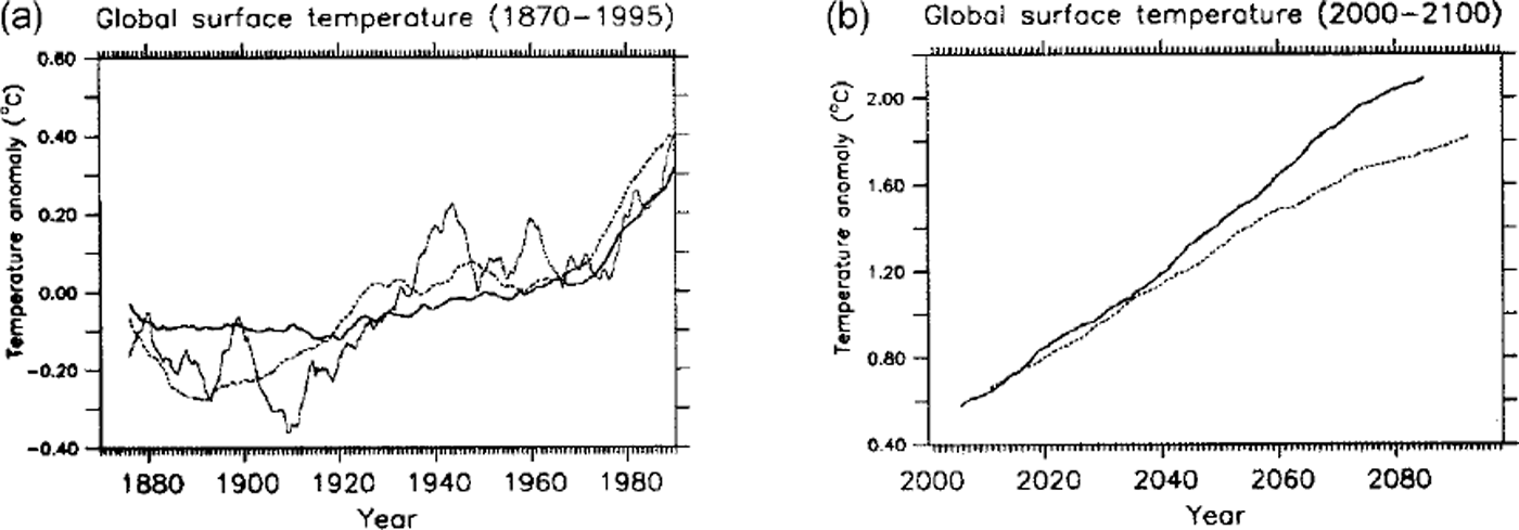
The global, ensemble mean surface air-temperature anomalies from the Historical and SV runs for 1870−1995 are shown in Figure 2a, with the observed global temperature anomalies from Reference Houghton, Callander and VarneyHoughton and others (1992). Both the Historical and SV runs show the warming ending in 1995 of about 0.5°C, similar to the observed values, with the greatest warming from 1980 through 1995. However, the observed warming of 0.5°C from 1910 through 1940 is not present in the Historical ensemble with the prescribed GHGSA. The SV ensemble, with solar flux increasing by almost 4 W m⁻² from 1890 to 1940, results in a global temperature increase of 0.35°C between 1890 and 1950. The solar flux after 1980 is about 1372 W m⁻², similar to that around 1940; however, both the modeled and observed temperatures after 1980 exceed the 1940 level.

Fig. 2. Globally averaged surface air-temperature anomalies (relative to 1870−1995 mean) for (a) PCM Historical (solid line) and sv (dashed line) ensemble averages, and intergovernmental panel on climate change temperature anomalies (dotted line) and (b) BAU (solid line) and stab (dashed line) temperature anomalies relative to the 1870−1995 mean of the historical run.

At first glance, these results suggest the hypotheses that (a) variable solar flux has contributed significantly to the periods of observed warming in the 20th century, and (b) the most recent observed warming is greater than that expected from the changes in solar flux, and may be attributable to increases in greenhouse gases. However, Reference Tett, Stott, Allen, Ingram and MitchellTett and others (1999) showed for the Hadley Centre GCM (HADCM2) simulations that the observed temperature trends could be attributed to greenhouse gases, sulfate aerosols and internal climate variability, without the variable solar flux. Similar regression analyses for the PCM simulations have not been performed, and simulations with only the variable solar flux would be required to determine their separate contribution to the modeled temperatures.

The ensemble-mean surface air-temperature anomalies for the BAU and Stab runs are shown in Figure 2b for the period 1995−2100, relative to the Historical period of 1870−1995. The Stab ensemble exhibits warming in 2080 of 1.8, and the BAU ensemble shows a warming of about 2.0°C.

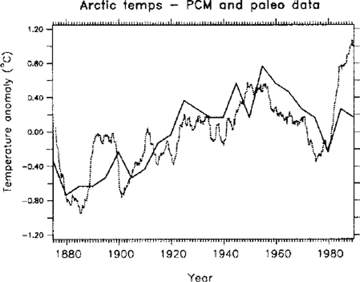
Arctic surface air-temperature anomalies from one of the SV simulations (not the ensemble average) are shown in Figure 3, superimposed on the Arctic temperature anomaly index derived by Reference OverpeckOverpeck and others’ (1997) proxy climate data that include lake varves, tree rings and ice cores. The modeled and the proxy temperatures show a similar warming of 1.4°C from 1880 to 1950, and a cooling of about 1.0°C from 1960 to 1980. The PCM shows an Arctic warming after 1980 of 1.4°C, while the proxy data warm only 0.4°C after 1980.

Fig. 3. Surface air-tem_perature anomalies (5 year running mean) in the arctic (70−90° N) from one sv run (dashed line), and the temperature anomaly index (solid line) derived from proxy data by Reference Overpeckoverpeck and others (1997).

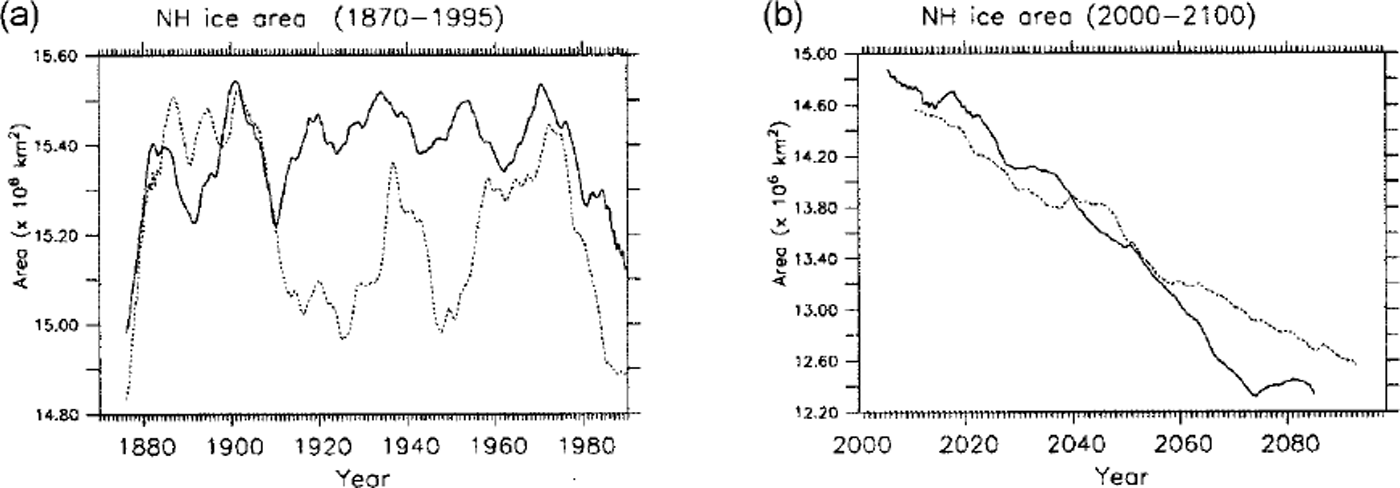
The sea-ice changes in the Northern Hemisphere (NH) as part of the global climate change are shown in Figures 3 and 4. NH total ice area (Fig. 4) shows variations of 0.5 × 10¹² m² over the period 1870−1980 only in the SVensemble, consistent with the periods of greater and lesser solar flux, and only a slightly larger decrease after 1980. The average thickness variations (Fig. 5) from 1870 through 1970 are about 0.10 m, and show a more pronounced trend after 1960, decreasing by about 0.16 m in both cases. The NH ice thickness continues to decrease by about 0.5 m in the 1995−2100 cases.

Fig. 4. Nh malice area ( × 1012 m2) in (a) the historical (solid) and SV (dashed) runs, and (b) the bau (solid) and stab (dashed) runs.

Fig. 5. Nh average ice thickness (m) in (a) the historical (solid line) and sv (dashed line) runs, and (b) the bau (solid line) and stab (dashed line) runs.

The downward trend in ice area appears strongly for both 1995−2100 runs, with an overall decrease of about 3 × 10¹² m². Ice thickness, however, shows a more significant change in the 20th century. However, one aspect of these PCM simulations is that, for present-day climate, the NH sea-ice area is about 25% larger than observed, as described in Weatherly and Zhang (in press). This large ice area is caused in part by biases in the atmospheric radiation leading to surface cooling. Shortwave radiation at the surface is up to 20 W m-² too low, attributable to larger-than-observed cloud optical thickness. Therefore, sea-ice cover in the Arctic Ocean would most likely be considerably smaller in response to greenhouse warming than that predicted with the PCM, perhaps with larger changes in regional temperatures and humidity. Ice thickness within the Arctic ice pack, however, decreases more rapidly after 1960 than this excessive ice area. The Southern Hemisphere sea ice exhibits significantly smaller change in both ice area and ice thickness in response to climatic changes from 1870 to 2100, similar to the interhemispheric asymmetry of the greenhouse response described by Reference Stouffer, Manabe and BryanStouffer and others (1989).

An analysis of the AO as represented in the PCM was performed, in which the empirical orthogonal functions (EOFs) of the seasonally averaged sea-level pressure (SLP) anomalies over the NH were computed from 200 years of the Control simulation of PCM for present-day climate (with constant GHGSA). The leading EOF pattern is shown in Figure 6, and resembles the AO as observed byReference Thompson and WallaceThompson and Wallace (1998). This is not necessarily a single coherent oscillation, but is two superimposed spatial patterns associated with the NAO and the Pacific-North American (PNA) pattern, as shown by the observational analysis by Reference DeserDeser (2000):

Fig. 6. First eof of winter seasonal slp anomalies from 200 years of pcm control simulation. contours are in 0.2 mbar intervals; negative contours are dashed.

The NAO signal (Arctic-Atlantic) and the PNA signal (Pacific-southeastern U.S.) are both strong, similar to observations. The Atlantic-Pacific correlation is stronger than observed, so the NAO and PNA signals are more synchronous in PCM than in reality. PCM also exhibits a stronger Pacific-Arctic correlation than observed, which suggests that either the Arctic responds more strongly in PCM to Pacific anomalies (like the El Niño-Southern Oscillation) or the Pacific SLP responds to the Arctic. This may explain why the PNA and NAO signals are more synchronous in PCM; the Pacific SLP is correlated to the Atlantic SLP because of its stronger correlation in the Arctic.

Conclusions

The Parallel Climate Model exhibits an AO in the winter-season SLP anomalies similar to those observed by Reference Thompson and WallaceThompson and Wallace (1998), and expresses the two distinct spatial patterns of the NAO and PNA that superimpose to form the AO, as found by Reference DeserDeser (2000). The PCM shows a greater signal correlated with the Pacific sector over the Arctic than is observed, which adds to the superimposed AO signal. It will require more GCM experiments to determine if this connection is related to the Arctic ice extent in PCM or other model dynamics.

The PCM climate simulations from 1870 through 1995 exhibit warming trends generally similar to those of global-average observations. They also agree with trends in the Arctic proxy climate data until about 1980, after which the PCM shows a strong warming trend not present in the proxy data. Ice thickness is shown to decrease by about 5% between 1960 and 1995. Analysis of submarine-based measurements of ice draft by Reference Rothrock, Yu and MaykutRothrock and others (1999) show a decrease of about −1.8 m during 1957−97, which is ten times greater than that simulated with PCM. NH ice area in the 20th century decreases by a less significant margin than the ice thickness, perhaps because the PCM has a bias toward excessive ice cover. Reference VinnikovVinnikov and others (1999) showed an accelerating decreasing trend in observed Arctic ice area, and showed that the observed trends parallel those simulated by the GFDL and HADCM2 GCMs. The PCM simulated ice-area trend parallels these two GCMs, though offset by the 25% bias in total ice area. Although PCM1 includes a high-resolution dynamic ice model with a complex rheology, it does not include a sophisticated thermodynamic model or an ice-thickness distribution. Its two-layer temperature model may not adequately resolve the thermal response of sea ice to perturbations. Improvements in sea-ice thermodynamics in global, coupled climate models may be required to accurately represent the response of sea ice to changes in greenhouse gases, solar forcing and natural variability.