2.1 Multiple hypotheses testing: Type I error probability control

As mentioned in the introduction, one way to increase the power to find a result of interest is simply to test more hypotheses in the same study. However, unless a proper multiple testing procedure is used, increasing the number of hypotheses tested typically leads to a larger Type I error probability. This is problematic since a goal of many designs is to keep this error under strict control at a certain prespecified level. The phenomenon can be illustrated by the following simple example. Suppose that m different null hypotheses are tested based on independent test statistics, and assume that the tests used have been chosen so as to make the individual (i.e., the nominal) Type I error probabilities equal to $\alpha$ . This means that the marginal probability to not reject a specific null hypotheses equals $1-\alpha$ , given that it is true and there is no non-zero effect. By the independence assumption, if all null hypotheses are true, then it follows that the probability to reject at least one of them is $1-{(1-\alpha )}^m$ . Hence, as m increases, the probability to falsely reject at least one null hypotheses converges to certainty.

To what extent it is important to keep the Type I error probability under strict control, and, if so, which significance level to choose, varies across scientific disciplines and applications. In order to choose appropriate values of the Type I error probability and power, one must weigh the value of correctly finding a positive effect against the loss of falsely declaring an effect as positive when it is not.

Before proceeding to discuss multiple testing procedures, note that there have been several different suggestions of how to generalise the concept of a Type I error probability for a single hypothesis to the case of multiple hypotheses. These are referred to as different error rates (see, e.g., Chapter 2 of Bretz et al. (Reference Bretz, Hothorn and Westfall2011)). Most relevant for the present paper is the FWER. Let $H_1,\dots ,H_m$ denote a set of m null hypotheses of interest, $m_0$ of which are true. The FWER is then defined as the probability of making at least one Type I error. This probability depends on the specific combination of hypotheses that are actually true, which of course is unknown when planning the experiment.

Multiple testing procedures for controlling the FWER are based on the concept of intersection hypotheses. Given the m individual hypotheses $H_1,\dots ,H_m$ and a non-empty subset of indices $I\subseteq \{1,\dots ,m\}$ , the intersection hypothesis $H_I$ is then defined as

(1) $\begin{array}{c}{H}_I=\bigcap _{i\in I}{H}_i,I\subseteq \{1,\dots ,m\}.\end{array}$

Local control of the FWER at level $\alpha$ for a specific intersection hypothesis $H_I$ holds when the conditional probability to reject at least one hypothesis given $H_I$ is at most $\alpha$ , i.e. when

(2) $\begin{array}{c}{P}_{H_I}\left(\text{Reject},,H_i,,,\text{for some},,i,\in ,I\right)\le \alpha .\end{array}$

Strong control of the FWER means that the inequality in Eq. (2) must hold for all possible non-empty subsets I. This more conservative requirement bounds the probability of making at least one Type I error regardless of which hypotheses are true. It is often deemed appropriate when the number of hypotheses is relatively small, while the consequences of making an error may be severe. There are a number of different multiple testing procedures available for local control of the FWER. One of the most widely applicable is the well-known Bonferroni procedure, which rejects $H_i$ at level $\alpha$ if the corresponding nominal test would have rejected $H_i$ at level $\alpha /m$ .

If a test has been defined for the local control of a collection of intersection hypotheses, strong control of the FWER can be attained by employing the closed testing principle. This principle states that if we reject an individual hypothesis $H_i$ if and only if all intersection hypotheses $H_I$ such that $i\in I$ are rejected at local level $\alpha$ , then the FWER is strongly controlled at level $\alpha$ (Marcus et al., Reference Marcus, Peretz and Gabriel1976). Since this principle is completely general with regards to the specific form of the tests for the intersection hypotheses $H_I$ , it follows that the choice of the local test will determine the properties of the overall procedure.

For many economic experiments, where multiple treatment groups are compared with one control group, a suitable test procedure for testing intersection hypotheses is the Dunnett test (Dunnett, Reference Dunnett1955). Using the closed testing principle, the Dunnet test can be used to obtain strong control over the FWER. The test is described in more detail in the Appendix.

2.2 Combined testing in adaptive designs

If we can look at some of the data before spending all available resources, then we could allocate the remaining samples to the most promising treatments. The present section contains a short introduction to the general topic of such adaptive designs, sufficient for the latter applications. As mentioned in the introduction, for reasons of clarity, we will limit ourselves to the case of two-stage designs with a single interim analysis. There are two main approaches. One is referred to as the combination test approach and was introduced by Bauer (Reference Bauer1989), and Bauer and Köhne (Reference Bauer and Köhne1994). The other, which makes use of conditional error functions, was introduced by Proschan and Hunsberger (Reference Proschan and Hunsberger1995) for sample size recalculation, while Müller and Schäfer (Reference Müller and Schäfer2004) widened the approach to allow for general design changes during any part of the trial.

Following Wassmer and Brannath (Reference Wassmer and Brannath2016), we assume for the moment that the purpose of the study is to test a single null hypothesis $H_0$ . We will see later how to combine interim adaptations with the closed testing principle when several hypotheses are involved. When the interim analysis is performed, there are two possibilities. Either $H_0$ is rejected solely based on the interim data $T_1$ from the first stage, or the study continues to the second stage, yielding data that we assume can be summarised by means of a statistic $T_2$ . In general, the null distribution of $T_2$ may then depend on the interim data. For instance, the first stage could inform an adjustment of the sample size of the second stage. Nevertheless, it is often the case that $T_2$ may be transformed so as to make the resulting distribution invariant with respect to the interim data and the adjustment procedure. In other words, the statistics used to evaluate the two stages will be independent given that $H_0$ is true, regardless of the interim data and the adaptive procedure.

As an example, suppose that $T_2$ is a normally distributed sample mean under $H_0$ , with mean 0 and a known variance ${\sigma }^2/n_2$ , with ${\sigma }^2$ being the variance of a single observation and $n_2$ a second stage sample size that depends on the interim data in some way. Then a one-sided p-value for the second stage can be obtained by standardising $T_2$ according to

(3) $\begin{array}{c}{p}_2=1-\Phi \left(\frac{T_2}{\sigma /\sqrt{n_2}}\right).\end{array}$

Assuming that the data from the two different stages is independent, it follows that the joint distribution of the p-values $p_1$ and $p_2$ from the two stages is known and invariant with respect to the interim adjustment. This is the key property which allows for the flexibility when choosing the adaptive design procedure.

Based on the conditional invariance principle, the design of an adaptive trial controlling the Type I error probability at a level $\alpha$ can be specified in terms of a rejection region for $p_1$ and a corresponding region for $p_2$ . This results in a sequential test of $H_0$ which is independent of the adaptation rule. The aforementioned main testing principles (combination tests and conditional error functions) only differ in the way the rejection region for the second stage is specified.

For the combination test approach, suppose that a one-sided null hypothesis $H_0:\theta \le 0$ . $\theta$ is some parameter of interest and is to be tested using a two-stage design with p-values $p_1$ and $p_2$ . The combination test procedure is specified in terms of three real-valued parameters, ${\alpha }_0$ , ${\alpha }_1$ and c, and a combination function $C(p_1,p_2)$ . It proceeds as follows:

1. 1. After the interim analysis, stop the trial with rejection of $H_0$ if $p_1\le {\alpha }_1$ and with acceptance of $H_0$ if $p_1>{\alpha }_0$ . If ${\alpha }_0<p_1\le {\alpha }_1$ , apply the adaptation rule and collect the data of the second stage.

2. 2. After the second stage, reject $H_0$ if $C(p_1,p_2)\le c$ and accept $H_0$ if $C(p_1,p_2)>c$ .

By virtue of the conditional invariance principle, it is easily shown that the Type I error probability is controlled at level $\alpha$ by any choice of ${\alpha }_0$ , ${\alpha }_1$ , c, and $C(p_1,p_2)$ satisfying

(4) $\begin{array}{c}{P}_{H_0}\left(\text{Reject},H_0\right)={\alpha }_1+{\int }_{{\alpha }_1}^{{\alpha }_0}{\int }_0^{1}1\left(C,(,p_1,,,p_2,),\le ,c\right)d{p}_{2}d{p}_1\le \alpha ,\end{array}$

where $1\left(·\right)$ denotes the indicator function. Naturally, ${\alpha }_1$ needs to be smaller than ${\alpha }_0$ . While specific values depend on the individual setting, Bauer and Köhne (Reference Bauer and Köhne1994, p.1031) argue that "a suitable value for ${\alpha }_0$ could be ${\alpha }_0=.5$ ". This corresponds to the situation that the effect goes in the right direction. If this value is chosen for ${\alpha }_0$ and the overall level of $\alpha$ is $\alpha =0.05$ , the remaining values are ${\alpha }_1=0.0233$ and $c=0.0087$ (see Table 1 in Bauer and Köhne (Reference Bauer and Köhne1994) for other typical threshold values). As a special case, if the first stage parameters of Eq. (4) are set to ${\alpha }_1=0$ and ${\alpha }_0=1$ , then there will be no early stopping (neither for futility nor with early success) and the null hypothesis will be rejected after the second stage if and only if $C(p_1,p_2)\le \alpha$ .

The other main approach, using conditional error functions, is very similar. The parameters ${\alpha }_0$ and ${\alpha }_1$ have the same role, but c and $C(p_1,p_2)$ are replaced by a conditional error function $A\left(p_1\right)$ such that, after the second stage, $H_0$ is rejected if $p_2\le A\left(p_1\right)$ and accepted if $p_2>A\left(p_1\right)$ . It is important to note that, as long as one of the procedures described above is followed, any type of rule can be used to update the sample size in an interim analysis. This means that not only can the information on efficacy collected so far be used in an arbitrary manner, but so can also any information external to the trial. For a more comprehensive review of the history and current status of adaptive designs as applied to clinical trials, see Bauer et al. (Reference Bauer, Bretz, Dragalin, König and Wassmer2016).

In the following, we only consider the inverse normal combination function (Lehmacher & Wassmer, Reference Lehmacher and Wassmer1999) for combining the p-values from the two stages. Although alternative choices exist it is commonly used and is the default method in the used software implementation. The definition of this function is

(5) $\begin{array}{c}C(p_1,p_2)=1-\Phi \left(w_1,{\Phi }^{-1},(1-p_1),+,w_2,{\Phi }^{-1},(1-p_2)\right),\end{array}$

where $w_1$ and $w_2$ are pre-specified weights that satisfy the requirement $w_1^2+w_2^2=1$ .Footnote ² With $p_1$ and $p_2$ independent and uniformly distributed, it follows from the definition that $C(p_1,p_2)$ becomes a random variable of the form $C(p_1,p_2)=1-\Phi \left(Z\right)$ , where Z follows a standard normal distribution. Thus, $C(p_1,p_2)$ can be treated as a p-value that combines the information from the two stages.

2.3 Two stage designs and power simulations

Having briefly introduced the necessary components, we are now ready to describe the step-by-step procedure characterising the class of adaptive designs of interest.

1. 1. Define a set of one-sided, individual null hypotheses $H_1,\dots ,H_m$ corresponding to comparisons of treatment means ${\mu }_i$ against a common control ${\mu }_0$ (i.e., $H_i:{\mu }_i\le {\mu }_0$ ).

2. 2. Given the first stage data, apply Dunnett’s test and compute a p-value $p_1^I$ for each non-empty intersection hypothesis $H_I$ such that $I\subseteq \{1,\dots ,m\}$ .

3. 3. Apply a treatment selection procedure to the first stage data, for example by selecting a fixed number of the best treatments. This results in a subset $J\subseteq \{1,\dots ,m\}$ taken forward to the second stage.

4. 4. Given the second stage data, apply Dunnett’s test and compute a p-value $p_2^I$ for each non-empty intersection hypothesis $H_I$ such that $I\subseteq J$ .

5. 5. Compute combined p-values $p_c^I=C(p_1^I,p_2^I)$ using a normal combination function for each $I\subseteq J$ . Reject each $H_I$ at local level $\alpha$ for which $p_c^I\le \alpha$ . Finally, ensure strong control of the FWER at level $\alpha$ by applying the closed testing principle and rejecting the individual hypotheses $H_i$ satisfying $p_c^I\le \alpha$ for all $I\subseteq J$ such that $i\in I$ .

Note that this procedure assumes that those hypotheses dropped at the interim cannot be rejected in the final analysis. This leads to a conservative procedure with an actual Type I error probability that may be lower than the pre-specified level $\alpha$ (Posch et al., Reference Posch, Koenig, Branson, Brannath, Dunger-Baldauf and Bauer2005).

There are a number of selection rules, which can be applied in this procedure. For example a fixed number (s) of treatments can be taken forward from the first to the second stage, e.g. the single best ( $s=1$ ) or the two best treatments ( $s=2$ ). Alternatively, the number of treatments taken forward can be flexible, either taking all treatments within a given range from the best treatment forward ( $ϵ$ -rule), or all treatments with a effect estimate at the interim analysis larger than a given threshold. Assuming that in most applications, the total sample size will be fixed due to budget reasons or a limited sample pool, specifying the number of treatments taken forward will often be a sensible choice, as it allows to determine the second stage sample size in the design phase.

Before an experiment is carried out, researchers usually want to investigate its statistical power. For adaptive approaches like the ones outlined above, these analyses build on simulations. All simulations presented in the remainder of the paper were carried out using the open source R package asdFootnote ³. This simulation package was originally developed for evaluating two-stage adaptive treatment selection designs using Dunnett’s test (Parsons et al., Reference Parsons, Friede, Todd, Marquez and Chataway2012), and was later extended to also support adaptive subgroup selection (Friede et al., Reference Friede, Stallard and Parsons2020).

After the treatments have been chosen for consideration in the experiment, the power simulations, as all power analyses, require prior beliefs about the expected effect sizes of the treatments. Further, the researcher needs to specify the number of observations in the different stages of the experiment and the selection rule (i.e. the numbers of groups which transfer to the second stage). The core idea for the simulation is to directly simulate the test statistics for the following hypothesis test, rather than individual observations (see Parsons et al., Reference Parsons, Friede, Todd, Marquez and Chataway2012; Friede et al.,Reference Friede, Parsons, Stallard, Todd, Valdes Marquez, Chataway and Nicholas2011 for details). Using a large number of drawn test statistics then allows to assess the expected power. The asd package, designed for these purposes, handles the issue of strong control of the FWER. A practical example of the simulation procedure is given in the following section. Additionally, a more principled discussion of the simulation procedure can be found in the supplementary material.

3.1 Application 1: Design of a field experiment

For the scenario outlined in the introduction, imagine that after consultations with stakeholders and colleagues, four potential treatments (+ one control) have been selected for consideration. Further, expected costs for data collection will allow for a total sample size of 300. For the present case, the project group may agree that standardized (Cohen’s d) effect sizes of 0.2, 0.2, 0.4 and 0.5 could reasonably be expected for the four treatments, implying that the group thinks that it is realistic that two of the treatments have small sized effects, and that the other two have medium sized effects (noted as "basic" scenario in the following).

One straightforward adaptive design would be that an interim analysis is carried out after 50% of the sample is collected and only the two best treatments are taken forward (implying a group size of 30 observations in the first stage, and 50 in the second stage). In a standard, non-adaptive experiment, the results of an interim analysis would not have any effect on the subsequent data collection, meaning that all four treatments are to be included in the second stage of the data collection. Thus, the power of both such experiments can be simulated with the asd-packageFootnote ⁴. Using 10,000 simulations shows that, for the standard design, the power of the experiment to reject at least one of the four Null hypotheses would be 62.27 % (Table 1). Such a design would conventionally be considered to be under-powered.

Table 1 Power simulation for the single stage design

Treatment	Assumed effect size	Selection of the treatment at stage 1 (%)	Hypothesis rejection at endpoint (%)
T1	0.2	100	12.87
T2	0.2	100	12.64
T3	0.4	100	37.72
T4	0.5	100	55.33

Power to reject H1 and/or H2 and/or H3 and/or H4 = 62.27%

In contrast, when only the two most promising treatments are carried over to the second stage after the interim analysis, the expected power to reject at least one of the Null hypotheses increases up to close to the conventional 80 % threshold (79.21 %, Table 2).

Table 2 Power simulation for the two stage design

Treatment	Assumed effect size	Selection of the treatment at stage 1 (%)	Hypothesis rejection at endpoint (%)
T1	0.2	23.02	6.85
T2	0.2	22.02	6.24
T3	0.4	69.65	45.05
T4	0.5	85.31	67.79

Power to reject H1 and/or H2 and/or H3 and/or H4 = 79.21 %

This serves as a first illustration of one of the potential benefits of the adaptive designs: given a fixed sample size, the power to reject at least one of the Nulls is substantially increased. Of course, this represents only one potential design. For example, it may be possible to find a design which also achieves an acceptable level of power, but requires a smaller total sample size, by changing the group size in the first stage. The left side of Fig. 1 shows the relationship between the first stage group size and the total sample size required to achieve 80 % power for rejecting at last one hypothesis. The right side shows the required sample size if the goal would be the rejection of the treatment with the largest assumed effect size (T4)Footnote ⁵.

Fig. 1 Total sample sizes to achieve 80% power in the basic scenario, for different first stage group sizes; Note: The dashed line indicates the sample size when no treatment selection is carried out

Figure 1 shows that, compared to a single stage design, the required sample size can be decreased in both cases. The required sample size to reject at least one null hypothesis can be reduced to 67 % of the original sample size. When the interest would be solely on rejecting the Null for the largest expected effect, the required minimum sample size is higher, but there is a 16 % reduction in comparison to the non-adaptive sample size. It is noteworthy that when the interest is only to reject the null hypothesis for the largest effect (T4), the group size of the first stage almost doubles, compared to when only aiming to reject one of the null hypotheses (around 40 in the former and around 20 in the latter case; compare the positions of the minima for the total sample sizes in Fig. 1).

Table 3 Effect size assumptions used in the power simulations

Scenario	T1	T2	T3	T4
Basic	0.2	0.2	0.4	0.5
Alternative I	0.1	0.1	0.2	0.5
Alternative II	0.1	0.1	0.5	0.8

As in other power analyses, the outcomes crucially depend on the assumptions about the expected effect sizes. To illustrate this, assume that there are two alternative sets of assumptions about the expected effect sizes held by different groups of researchers (“Alternative I” and “Alternative II”), depicted in Table 3. One group may believe that the “small” effect sizes are actually smaller and the medium effect sizes are more “distinct” than in the basic scenario (“Alternative 1”), while another group may argue that the two treatments will only have small effects, one a medium and the last one a large effect. The required sample sizes of these sets can be simulated for the basic scenario and are depicted in Figs. 2 and 3.

Fig. 2 Total sample sizes to achieve 80% power in scenario “Alternative I”, for different first stage group sizes; Note: The dashed line indicates the sample size when no treatment selection is carried out

The difference between the expected effect sizes of T3 and T4 in scenario Alternative I is larger than in the basic scenario. At the same time, the expected effect sizes for T1, T2 and T3 are smaller than in the basic scenario (cf. Table 3). This leads to overall larger required sample sizes for Alternative 1, both for single stage designs and two-stage designs (for most of the considered first stage group sizes, compare Figs. 1 and 2). Still, the expected savings in sample size are 33% and 31%, and both optimal group sizes in the first stage around 20–25 observations (cf. the minimum of the solid line in Fig. 2). The assumptions for Alternative II, which include one large expected effect, lead to substantially smaller sample sizes than the basic scenario, for all considered designs (compare Figs. 1 and 3). Still, using an adaptive design allows saving a substantial share of the required total sample size (respectively 35% and 32%).

These simulation results show that the required sample size for a two-stage design could be reduced by about 30% compared to a single-stage design. Still, the sample size savings vary for the different assumptions regarding the effect sizes. It has also be noted that this requires that the group size in the first stage is appropriately chosen; see discussion below.

Fig. 3 Total sample sizes to achieve 80% power in scenario “Alternative II”, for different first stage group sizes; Note: The dashed line indicates the sample size when no treatment selection is carried out

3.2 Application 2: A business management game for regulatory impact analysis

To further illustrate the application of the adaptive designs, we apply a two-stage design to the experiment of Musshoff and Hirschauer (Reference Musshoff and Hirschauer2014). Here, rather than simulating the experiment, a subset of the actual data from the experiment is used. In their experiment, the impact of four different nitrogen reduction policies on the decision-making of the participants is investigated and compared to a base case. The participants play a multi-period, single-player business simulation game. The sample consists of data from 190 agricultural university students, taking on the role of farmers deciding on a production plan for a hypothetical crop farm. Each individual plan specifies the land usage shares for the different crops, as well as the amount of nitrogen fertiliser to be used. The objective of each player is to maximise his or her bank deposit at the end of the 20 production periods that make up the total game time.

In the first 10 production periods, all players receive an unconditional, governmental deterministic agricultural payment. After these initial periods, the players are randomly assigned to one of five different policy scenarios. The first scenario can be interpreted as “business as usual”, in which the deterministic payments are continued. The other four are actual interventions, designed to foster more environmentally friendly production. They differ with respect to whether payments are granted (scenario 2 and 3), or whether penalties are charged (scenario 4 and 5) when the fertiliser usage is respectively above or below a given threshold (voluntary vs. prescriptive). Further, they vary in terms of whether the payments or penalties are made without exception (scenario 2 and 4), or whether there is only a certain probability that a player’s action is discovered and payments or penalties are applied (scenario 3 and 5; deterministic vs. stochastic). The scenario designs ensure the same expected monetary gain for the players (see Sect. 3 of Musshoff and Hirschauer, Reference Musshoff and Hirschauer2014 for a detailed description of the experiment).

The main outcome variable of interest is the share of arable land where the players kept the fertiliser levels below a pre-specified threshold referred to as “extensive use”, defined to be 75 kg per hectare. In the first ten periods the group mean shares were similar, all between 11.6% and 17.4%. For periods 11 to 20 the shares were, for scenario 1 to 5 in order, 13.6%, 67.5%, 80.7%, 80.9% and 49.4% (see Table 4 of Musshoff and Hirschauer, Reference Musshoff and Hirschauer2014). Thus, scenarios 2-5 yield much higher share values compared to the reference scenario, and moreover these seem to lead to different outcome means although they all give the same expected profit.

Here, we focus on the subset of data corresponding to scenarios 2, 3 and 4. For each of these groups, there is data for 38 players. As the total sample size increases in the examples below, more and more players are used from each group, in the order they are included in the original data file.Footnote ⁶ We use scenario 2 as the control (rather than scenario 1) and treat 3 and 4 as two different active treatments (treatment 1 and 2). We may interpret this as a smaller study in which a deterministic penalty (scenario 3) and a stochastic penalty (scenario 4) are compared against a deterministic reward (scenario 2). The subset is chosen for illustrative purposes, but is also in close correspondence with one of the original hypotheses of Musshoff and Hirschauer (Reference Musshoff and Hirschauer2014). The null hypothesis for the comparison of scenario 3 vs. 2 is denoted by $H_1$ , while the one corresponding to 4 vs. 2 is denoted by $H_2$ . While scenario 2 (as a policy intervention) would be preferable based on equality arguments, high monitoring costs may make it impractical and warrant alternative interventions. Such are provided by scenarios 3 and 4, but which of them works best when taking into account the multiple goals (e.g. income and environment concerns) and bounded rationality of an economic decision maker?

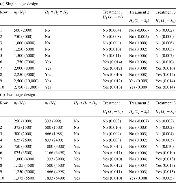
Tables 4a and b provide a comparison showing which hypotheses are rejected for different subsets of the data. As in the previous subsection, groups within the same stage are always of equal size. The subset of the data used consists of one control and two treatment groups (treatment 1 and 2). Thus, the selection rule at the interim analysis study takes only the better active treatment forward. As in the basic scenario in Application 1, approximately half the total sample size is used in the first stage. This design was chosen since it was found to be close to optimal in the simulations performed. It can be observed that the two-stage design is able to reject at least one hypothesis (namely, $H_1$ ) once the total sample size N becomes large enough (row 6 and 7 in Table 4b), while the single-stage design never rejects any hypothesis. Hence, the adaptive design increases the power of detecting at least one effect by dropping one scenario at the interim analysis and focusing on the one that seems to have the largest effect.

Table 4 Hypotheses rejected in Dunnett tests for single- and two-stage designs of increasing sizes, together with mean difference estimates of effect sizes.

(a) Single-stage design
Row	$n_1\left(N_1\right)$	$H_1\cap H_2$		Treatment 1	Treatment 2
				$H_1({\overline{x}}_1-{\overline{x}}_0)$	$H_2({\overline{x}}_2-{\overline{x}}_0)$
1	10 (30)	No		No (8.00)	No (39.30)
2	13 (39)	No		No (35.38)	No (32.54)
3	16 (48)	No		No (32.31)	No (25.63)
4	20 (60)	No		No (36.65)	No (55.75)
5	23 (69)	No		No (39.04)	No (50.22)
6	26 (78)	No		No (41.38)	No (53.19)
7	30 (90)	No		No (55.03)	No (52.60)

(b) Two-stage design
Row	$n_1\left(N_1\right)$	$n_2\left(N_2\right)$	$H_1\cap H_2$	Treatment 1	Treatment 2
				$H_1({\overline{x}}_1-{\overline{x}}_0)$	$H_2({\overline{x}}_2-{\overline{x}}_0)$
1	5 (15)	7 (14)	No	No (12.83)	No (64.42)
2	7 (21)	9 (18)	No	No (24.28)	No (25.63)
3	9 (27)	11 (22)	No	No (30.77)	No (55.75)
4	10 (30)	15 (30)	No	No (39.00)	No (53.72)
5	12 (36)	17 (34)	No	No (22.24)	No (49.07)
6	14 (42)	19 (38)	Yes	Yes (60.67)	No (29.51)
7	15 (45)	22 (44)	Yes	Yes (58.57)	No (36.00)

Note that the total sample sizes for the corresponding rows of Tables 4a and b have been selected to be as close as possible. Type I error probability $\alpha =0.025$ . $n_1$ = first stage group size, $n_2=$ second stage group size. $N_1=$ total first stage sample size, $N_2=$ total second stage sample size

3.3 Application 3: A field experiment in charitable giving behaviour

Last, we consider the study of Karlan and List (Reference Karlan and List2007), which is concerned with the effect of a matching grant on charitable giving. A matching grant represents an additional donation made by a central donor backing the study, the size of which depends on the amount donated by the regular donors. The sample consists of data from 50,083 individuals, who were identified as previous donors to a non-profit organisation and were contacted by mail.

Two thirds of the study participants were assigned to some active treatment group, while the rest were assigned to a control group. The active treatments varied along three dimensions: (1) the price ratio of the match ($1:$1, $2:$1 or $3:$1)Footnote ⁷; (2) the maximum size of the matching gift based on all donations ($25,000, $50,000, $100,000 or unstated) and (3) the donation amount suggested in the letter (1.00, 1.25 or 1.50 times the individual’s highest previous contribution). Each of these treatment combinations was assigned with equal probability. The authors study both the effects on the response rate as well as the donation amount. However, we will only focus on how the matching ratio affects the response rate. The reason for this simplification is that we want to be able to connect the simulation results in the previous section to the available real-world data without increasing the complexity of the presentation by introducing too many treatment groups.

For illustrative purposes, we will only consider a portion of the data analysed by Karlan and List (Reference Karlan and List2007). Specifically, we will restrict ourselves to the subset consisting of those individuals residing in red states (i.e., states with a republican majority, see Panel C of Table 2A of Karlan and List, Reference Karlan and List2007). The reason for this is that, as noted by Karlan and List (Reference Karlan and List2007), it is only for this subgroup that the original analysis shows a statistically significant difference between the groups defined by the different matching ratios. Naturally, a real analysis would not ignore data just because it is not statistically significant. However, since our purpose here is to compare methods of data analysis rather than to answer specific research questions, we choose to restrict ourselves to a subset in order to be able to more clearly highlight the difference between the single-stage and two-stage designs. Thus, there are three active treatments, corresponding to the different matching ratios. Again, the sample size is divided equally among the groups in each stage, but we employ a rule that selects the two best treatments at the interim analysis, in contrast to the previous application.

Table 5 Hypotheses rejected in Dunnett tests for single- and two-stage designs of increasing sizes, together with mean difference estimates of effect sizes

(a) Single-stage design
Row	$n_1\left(N_1\right)$	$H_1\cap H_2\cap H_3$		Treatment 1 $H_1({\overline{x}}_1-{\overline{x}}_0)$	Treatment 2	Treatment 3
					$H_2({\overline{x}}_2-{\overline{x}}_0)$	$H_3({\overline{x}}_3-{\overline{x}}_0)$
1	500 (2000)	No		No (0.004)	No (-0.006)	No (0.002)
2	750 (3000)	No		No (0.008)	No (-0.005)	No (0.000)
3	1,000 (4000)	No		No (0.009)	No (0.000)	No (0.006)
4	1,250 (5000)	No		No (0.010)	No (0.002)	No (0.005)
5	1,500 (6000)	No		No (0.011)	No (0.006)	No (0.007)
6	1,750 (7000)	Yes		Yes (0.014)	No (0.008)	No (0.010)
7	2,000 (8000)	Yes		Yes (0.012)	No (0.008)	Yes (0.010)
8	2,250 (9000)	Yes		Yes (0.010)	No (0.008)	Yes (0.012)
9	2,500 (10,000)	Yes		Yes (0.012)	Yes (0.009)	Yes (0.014)
10	2,750 (11,000)	Yes		Yes (0.013)	Yes (0.009)	Yes (0.014)

(b) Two-stage design
Row	$n_1\left(N_1\right)$	$n_2\left(N_2\right)$	$H_1\cap H_2\cap H_3$	Treatment 1	Treatment 2	Treatment 3
				$H_1({\overline{x}}_1-{\overline{x}}_0)$	$H_2({\overline{x}}_2-{\overline{x}}_0)$	$H_3({\overline{x}}_3-{\overline{x}}_0)$
1	250 (1000)	333 (999)	No	No (0.003)	No (-0.007)	No (0.002)
2	375 (1500)	500 (1500)	No	No (0.010)	No (0.003)	No (0.002)
3	500 (2000)	666 (1988)	No	No (0.009)	No (0.003)	No (0.004)
4	625 (2500)	833 (2499)	No	No (0.009)	No (0.002)	No (0.005)
5	750 (3000)	1000 (3000)	Yes	Yes (0.014)	No (0.005)	No (0.010)
6	875 (3500)	1166 (3498)	Yes	Yes (0.011)	No (0.006)	Yes (0.010)
7	1,000 (4000)	1333 (3999)	Yes	Yes (0.010)	No (0.004)	Yes (0.013)
8	1,125 (4500)	1500 (4500)	Yes	Yes (0.012)	No (0.004)	Yes (0.013)
9	1,250 (5000)	1666 (4998)	Yes	Yes (0.011)	No (0.003)	Yes (0.013)
10	1,375 (5500)	1833 (5499)	Yes	Yes (0.010)	Yes (0.008)	No (0.005)

Note that the total sample sizes for the corresponding rows of Tables 5a and 5b have been selected to be as close as possible. Type I error probability $\alpha =0.025$ . $n_1$ = first stage group size, $n_2=$ second stage group size. $N_1=$ total first stage sample size, $N_2=$ total second stage sample size

Comparing Table 5a with b, it can be seen that the single-stage design rejects no hypothesis up until a total sample size of $N_1=7000$ (row 6 in Table 5a). In contrast, the two-stage design starts to reject a hypothesis, namely $H_1$ (treatment 1), from $N_1+N_2=6000$ (row 5 in Table 5b), indicating the potential reduction to sample size by 1000 observations.