2.1. Numerical configuration

The dataset used for the quantification of mixing was derived from the direct numerical simulation (DNS) conducted by Zhou (Reference Zhou2022), henceforth referred to as Z22. Detailed descriptions of the simulation are provided in Z22. The numerical configuration aims to replicate the laboratory experiments of Spedding (Reference Spedding1997). These experiments examined the turbulent wake of a sphere of diameter $D$, towed at speed $U_0$ in a fluid with a uniform buoyancy frequency $N$, as illustrated in figure 1. Employing a spectral multidomain method (Diamessis et al. Reference Diamessis, Domaradzki and Hesthaven2005), the simulation solves the incompressible Navier–Stokes equations under the Boussinesq approximation. Zhou & Diamessis (Reference Zhou and Diamessis2019), hereafter ZD19, conducted large-eddy simulations (LES) spanning a broad range of wake Reynolds and Froude numbers, ${\textit {Re}} \equiv U_0D/\nu$ and ${\textit {Fr}} \equiv 2U_0/ND$. In contrast, Z22 conducted a DNS focusing on a specific case with $({\textit {Re}},{\textit {Fr}})=(25\,000,4)$, generating the dataset for the present analysis. This specific parameter set was selected for its ability to access the strongly stratified dynamics while being computationally feasible. The Prandtl number was set to one in this simulation.

Figure 1. Schematic of the computational domain for a temporally evolving, stably stratified wake behind a towed sphere (Diamessis, Domaradzki & Hesthaven Reference Diamessis, Domaradzki and Hesthaven2005; Diamessis, Spedding & Domaradzki Reference Diamessis, Spedding and Domaradzki2011). The mean flow is along the $x$-direction, and the wake's centreline is at $(y,z)=(0,0)$.

Although the simulation models a sphere wake, it does not explicitly compute flow around an object. Instead, the wake is configured to evolve temporally (Orszag & Pao Reference Orszag and Pao1975), and the sphere's impact on the flow is mimicked through a sophisticated scheme (Diamessis et al. Reference Diamessis, Spedding and Domaradzki2011) that creates an initial condition presenting the self-similar flow profiles in the near wake (Spedding Reference Spedding1997). This initial condition corresponds to a downstream distance at which the instabilities initiated by the sphere motion have fully developed, and self-similarity in terms of the mean and fluctuation quantities has been established in the flow (see details in § 3 of Diamessis et al. Reference Diamessis, Spedding and Domaradzki2011). While simulations including the sphere have become feasible in recent years (e.g. Orr et al. Reference Orr, Domaradzki, Spedding and Constantinescu2015; Pal et al. Reference Pal, Sarkar, Posa and Balaras2017), such sphere-less simulations remain the workhorse for investigating turbulent wakes at large ${\textit {Re}}$ (see a recent survey by Li, Yang & Kunz Reference Li, Yang and Kunz2024). Once the sphere-less wake flow simulation begins, it proceeds without any external forcing besides buoyancy, leading to an unforced stratified flow decaying naturally from a fully turbulent initial state. The sphere's direct impact is incorporated into the initial condition and does not persist during the main wake simulation. This configuration is analogous to the decaying homogeneous turbulence scenario explored by de Bruyn Kops & Riley (Reference de Bruyn Kops and Riley2019) (hereafter dBKR19) but with pronounced inhomogeneity across the plane orthogonal to the mean flow direction, i.e. the $y$–$z$ plane (figure 1).

2.2. Evolution of wake turbulence

The inhomogeneity over the $y$–$z$ plane leaves only one statistically homogeneous direction in the flow, i.e. the $x$-direction. Applying Reynolds decomposition to the velocity field, $\boldsymbol {U}$, along the $x$-direction yields

(2.1)\begin{equation} \boldsymbol{U}(\boldsymbol{x},t)=(\langle U\rangle_{x},0,0)+(U',V',W'), \end{equation}

where $\langle {\cdot } \rangle _x$ denotes an average in the $x$-direction, and $\boldsymbol {U}'\equiv (U',V',W')$ is the fluctuation velocity. Other than internal waves generated by the wake turbulence (Zhou & Diamessis Reference Zhou and Diamessis2016; Rowe, Diamessis & Zhou Reference Rowe, Diamessis and Zhou2020), the fluid is essentially quiescent in the wake's surroundings. Following ZD19, the core region of the wake is defined to be within an elliptic cylinder centred around the wake's centreline, i.e.

(2.2)\begin{equation} \frac{y^2}{(2L_H)^2}+\frac{z^2}{(2L_V)^2}\le1, \end{equation}

where $L_H$ and $L_V$ are the characteristic width and height of the mean wake, respectively. Quantities can be averaged for the wake's core region as defined above, and we will use $\langle {\cdot } \rangle$ to denote such a volume average.

The choice to define the boundary using (2.2) was guided by visual inspections similar to those presented in figure 7 of Z22, where the above definition leads to a reasonably accurate demarcation of the turbulent/non-turbulent (T/NT) interface. The dimensions of $L_H$ and $L_V$ are dynamically adjusted in accordance with changes in the mean flow profile, ensuring that they accurately represent the shape and scale of the mean wake over time. This simple definition does not present the finer details of the T/NT interface should it be defined using more sophisticated criteria (e.g. Watanabe et al. Reference Watanabe, Riley, de Bruyn Kops, Diamessis and Zhou2016) and could introduce a modest degree of uncertainty in the bulk estimates. We anticipate this uncertainty to be relatively minor compared with those introduced by the inherent intermittency of the turbulence, i.e. averaging over dynamically distinct patches to obtain bulk statistics. To address this limitation, a conditional sampling approach is developed in § 4.

Key to describing the mixing efficiency is the dissipation rate of TKE, $\varepsilon$, and the destruction rate of buoyancy variance, $\chi$:

(2.3a,b)\begin{equation} \varepsilon(\boldsymbol{x},t)\equiv 2\nu S'_{ij}S'_{ij},\quad\chi(\boldsymbol{x},t)\equiv\frac{\kappa}{N^2}\frac{\partial b'}{\partial x_i}\frac{\partial b'}{\partial x_i}. \end{equation}

Here, $S'_{ij}\equiv (1/2)(\partial U'_i / \partial x_j + \partial U'_j / \partial x_i)$ is the rate of strain tensor due to $\boldsymbol {U}'$, and $b'$ is the buoyancy fluctuation. The volume-averaged $\varepsilon$ within the wake core, $\langle \varepsilon \rangle$, determines two fundamental length scales of the stratified turbulence, $\ell _K\equiv ({\nu ^3}/{\langle \varepsilon \rangle })^{1/4}$ and $\ell _O\equiv (\langle \varepsilon \rangle /{N^3})^{1/2}$, the Kolmogorov and Ozmidov scales, respectively.

Dynamical insights can be obtained by examining the time evolution of $\ell _O$ and $\ell _K$, alongside the horizontal and vertical integral length scales of turbulence, $\ell _h$ and $\ell _v$, all plotted in figure 2(a). (The procedure of estimating $\ell _h$ and $\ell _v$ is documented in appendix C of ZD19.) Here, $\ell _h$ is consistently larger than $\ell _v$, highlighting the strong anisotropy within the energy-containing, large-scale turbulent structure. As demonstrated by ZD19, $\ell _h$ can be considered as the typical size of the ‘pancake’ vortices (Spedding Reference Spedding1997), and $\ell _v$ is the characteristic length associated with the shear layers that spontaneously form due to strong stratification (Diamessis et al. Reference Diamessis, Spedding and Domaradzki2011), which is a defining feature of the SST/LAST regime. The Ozmidov scale, $\ell _O$, indicative of the largest horizontal scale with adequate kinetic energy for overturning, initially significantly surpasses the viscous scale, $\ell _K$. Over time, as the turbulence decays, $\ell _O$ diminishes and $\ell _K$ enlarges. They intersect at $Nt\approx 27$, marking the end of the dynamic range between $\ell _O$ and $\ell _K$, and the onset of viscous control. In figure 2(b), we examine the evolution of the buoyancy Reynolds number and horizontal turbulent Froude number:

(2.4a,b)\begin{equation} \textit{Re}_b\equiv\frac{\langle \varepsilon \rangle}{\nu N^2}=\left(\frac{\ell_O}{\ell_K}\right)^{4/3},\quad \textit{Fr}_h\equiv\frac{\sqrt{\langle U'^2+V'^2 \rangle}}{N\ell_h}. \end{equation}

The value of ${\textit {Re}}_b$ is initially $\simeq 20$ at $Nt=1$ and drops below unity by $Nt\approx 27$, while ${\textit {Fr}}_h$ decreases from 0.033 to 0.007, indicating a stronger buoyancy control on the eddies of size $\ell _h$ as time progresses. The inset displays the time series of the vertical Froude number, ${\textit {Fr}}_v^{\star }\equiv 2{\rm \pi} \sqrt {\langle U'^2+V'^2 \rangle }/N\ell _v$. From wakes of varying ${\textit {Re}}$ and ${\textit {Fr}}$, ZD19 noted that a ${\textit {Fr}}_v^\star$ range of approximately 0.5 to 1 would indicate that buoyancy has reorganized the flow to establish a vertical scale $\ell _v$ following the self-similar scaling of Billant & Chomaz (Reference Billant and Chomaz2001) in the strongly stratified ${\textit {Fr}}_h\ll 1$ limit, leading to the predominance of layering dynamics within the turbulence. This period of $0.5\lesssim {\textit {Fr}}_v^\star \lesssim 1$ indeed occurs in this specific wake for $4\lesssim Nt \lesssim 30$ (see the inset of figure 2b), and we will refer to this period as the ‘strongly stratified’ or ‘layering’ phase of the wake turbulence.

Figure 2. (a) Length scales of dynamical significance, normalized by $D$, plotted against dimensionless time, $Nt$. (b) The path of wake turbulence within the $({\textit {Fr}}_h,{\textit {Re}}_b)$ space is shown by a thick grey line, with coloured symbols highlighting specific instances for analysis in § 4. Small grey triangles indicate a subset of simulations by Maffioli et al. (Reference Maffioli, Brethouwer and Lindborg2016). The inset to panel (b) shows the time series of the vertical Froude number, ${\textit {Fr}}_v^{\star }$.

2.3. Flow visualization

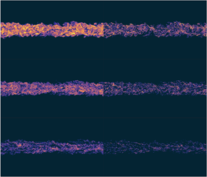
Previous visualizations of stratified wake flows primarily concentrated on vortical structures. For example, figure 4 of ZD19 demonstrated the spontaneous formation of spanwise vorticity layers, while Halawa et al. (Reference Halawa, Merhi, Tang and Zhou2020) examined how variations in ${\textit {Re}}$ influence potential vorticity structures. In figure 3, we shift our focus to the spatial distribution of $\varepsilon$ and $\chi$ over the centre $oxz$ plane at various stages of wake turbulence corresponding to those highlighted in figure 2(b). In general, $\varepsilon$ exhibits higher intensity than $\chi$. Both variables display significant spatial intermittency, with their magnitudes changing abruptly over very small length scales. Over time, the intensities of both $\varepsilon$ and $\chi$ diminish, with the decline in $\varepsilon$ leading to an increase in Kolmogorov length and a decrease in Ozmidov scale (figure 2a). Consequently, the bulk ${\textit {Re}}_b$ decreases and the dynamic range below $\ell _O$ and above $\ell _K$ shrinks. At instance A, i.e. $Nt=2$, when ${\textit {Re}}_b=19$ and turbulence is vigorous, high-intensity regions of $\varepsilon$ and $\chi$ are distributed uniformly in the flow. By instance C, i.e. $Nt=10$, the bulk ${\textit {Re}}_b$ has dropped to approximately 4.3, and the high-intensity ‘filaments’ of $\chi$ have become markedly sparser. These filaments tend to display opposing orientations on either side of the wake centreline ($z=0$), aligning with the mean shear within the wake.

Figure 3. Vertical transects at the centre $oxz$ plane ($y=0$; see figure 1) of (a i,b i,c i) $\log _{10}\varepsilon$ and (a ii,b ii,c ii) $\log _{10}\chi$ at selected time instances A–C highlighted in figure 2(b). The images shown are close-up views for $(-10/3)D< x<(10/3)D$ and $(-4/3)D< z<(4/3)D$. The towed sphere generating this wake moves from left to right in the positive $x$ direction (see figure 1).

3.1. $\langle \varepsilon \rangle$, $\langle \chi \rangle$ and $\varGamma$

Figure 4(a) illustrates the temporal evolution of the volume-averaged values of $\varepsilon$ and $\chi$. Here, $\langle \varepsilon \rangle$ exhibits a monotonic decrease, while $\langle \chi \rangle$ initially rises, levels off briefly for $2\lesssim Nt \lesssim 3$ and then decreases. The decay rate for $\varepsilon$ appears to accelerate at $Nt\approx 4$. These patterns align, at least qualitatively, with dBKR19's data on decaying homogeneous turbulence in their figure 7. In dBKR19, turbulence decays from both comparable (Cases I and II) and higher (Cases III and IV) values of ${\textit {Re}}_b$, while their ${\textit {Fr}}_h$ values are considerably higher than ours.

Figure 4. Time series of (a) $\langle \varepsilon \rangle$ and $\langle \chi \rangle$, both normalized by $U_0^3/D$, (b) $\varGamma$, (c) $\ell _O$ and $\ell _T$, both normalized by $D$, and (d) $\ell _O/\ell _T$. Grey dash-dotted lines in panels (a,b) indicate $Nt=5$ and $13$, respectively.

Time series of the flux coefficient, $\varGamma =\langle \chi \rangle /\langle \varepsilon \rangle$, is presented in figure 4(b). Initially, $\varGamma$ starts at a low value of 0.09 at $Nt=1$. As buoyancy effects become more dominant and the wake turbulence enters the layering phase, $\varGamma$ increases quickly and reaches a plateau by $Nt\approx 5$. The value of $\varGamma$ fluctuates weakly within 0.45–0.49 before it begins a steady decline after $Nt=13$. In their homogeneous turbulence study, dBKR19 observed a period in which $\varGamma$ only weakly oscillates with time before it drops (see their figure 8). The present wake data suggest peak $\varGamma$ values of 0.45–0.49, comparable to the asymptotic value (at large ${\textit {Re}}_b$) of 0.54 observed by dBKR19. A comparison can also be drawn with the findings of Chongsiripinyo & Sarkar (Reference Chongsiripinyo and Sarkar2020), who conducted simulations of disk wakes at ${\textit {Re}}=5\times 10^4$. Their figure 20 indicates that while initially $\langle \chi \rangle \ll \langle \varepsilon \rangle$ in the near wake (implying $\varGamma \ll 1$), $\langle \chi \rangle$ gradually approaches while remains smaller than $\langle \varepsilon \rangle$ as the turbulence enters the SST regime, suggesting a plateauing $\varGamma$ value similar to that observed in the sphere wake.

3.2. Thorpe versus Ozmidov scales

A relevant length scale that characterizes the turbulent overturning events is the Thorpe scale, $\ell _T$, which has been explored in discussions on mixing efficiency (e.g. Smyth, Moum & Caldwell Reference Smyth, Moum and Caldwell2001; Mashayek, Caulfield & Peltier Reference Mashayek, Caulfield and Peltier2017). For the wake data, $\ell _T$ is determined by the root mean square of the vertical displacement ($\delta _T$) of fluid parcels from their equilibrium position in the ‘sorted’ density profile, i.e. $\ell _T\equiv \langle \delta _T^2 \rangle ^{1/2}$. We adopted the ‘sorting’ procedure of Mashayek et al. (Reference Mashayek, Caulfield and Peltier2017) (hereafter MCP17) to compute $\ell _T$ (or $L^{\textrm {3D}}_T$ in MCP17's notation).

We analyze the temporal evolution of $\ell _T$ alongside $\ell _O$ in figure 4(c). Unlike $\ell _O$, which exhibits a monotonic decay mirroring the trend in $\langle \varepsilon \rangle$ (figure 4a), $\ell _T$ increases between $Nt=1$ and 2, before subsequently decreasing. The peak of $\ell _T$ at $Nt=2$ is noteworthy, as it corroborates elements of Spedding (Reference Spedding1997)'s heuristic reasoning on the ‘non-equilibrium’ (NEQ) regime. During the transition from the fully turbulent early wake to the NEQ regime, Spedding noted a reduced decay rate in the mean centreline velocity $U_c$ (see his figure 7). Without density measurements, Spedding hypothesized that at $Nt\approx 2$, fluid parcels achieve their maximum displacement from the equilibrium position and start to ‘relax back’, thus converting available potential energy (APE) into kinetic energy and slowing down the mean flow's decay. That $\ell _T$ peaks at $Nt\approx 2$ provides direct evidence to this interpretation.

The time series of the ratio $\ell _O/\ell _T$ is shown in figure 4(d). Aside from a brief levelling off when the turbulence transitions to the layering phase around $Nt\approx 4$, $\ell _O/\ell _T$ exhibits an almost monotonic and considerably weak decline over time, maintaining a value below unity. This contrasts markedly with the scenario of the weakly stratified, KH-driven cases studied by MCP17, where $\ell _O/\ell _T$ begins at a low value of $O(0.1)$ and then increases rapidly as the KH billow rolls up and transitions to turbulence, eventually exceeding one, i.e. $\ell _O>\ell _T$. The pattern shown for the wake in figure 4 reverses the progression in time observed in the KH case: $\ell _T$, initially comparable to $\ell _O$, peaks early in the wake at $Nt\approx 2$ and then diminishes over time as fluid parcels gradually return to equilibrium, releasing the system's APE. The faster decay rate of $\ell _O$, driven by the rapid dissipation of TKE, results in an increasing separation between $\ell _T$ and $\ell _O$, which results in $\ell _O\le \ell _T$ for the entire time. The range of the $\ell _O/\ell _T$ ratio exhibited by this specific wake is relatively narrow, spanning from 0.3 to 1. In contrast, the shear layer cases investigated in MCP17 showed a wider range of $\ell _O/\ell _T$ ratios, from approximately 0.1 to 10 (e.g. see their figure 6).

3.3. Parametrization of $\varGamma$

In a seminal paper, Shih et al. (Reference Shih, Koseff, Ivey and Ferziger2005) introduced a scaling for $\varGamma$ based on ${\textit {Re}}_b$. Later, Ivey, Winters & Koseff (Reference Ivey, Winters and Koseff2008) suggested that additional parameters might be necessary to capture the complexities in the flow, such as intermittency. The wake data, shown in figure 5(a), are categorized into the ‘molecular’ and ‘transitional’ regimes according to the ${\textit {Re}}_b$-based scaling. For these regimes, Bouffard & Boegman (Reference Bouffard and Boegman2013) revised the $\varGamma$–${\textit {Re}}_b$ scaling using field data (see their figure 9). Although the wake data exhibit the anticipated increasing trend with ${\textit {Re}}_b$ for ${\textit {Re}}_b\lesssim 3$, the peak $\varGamma$ values, ranging from 0.45 to 0.49, are considerably higher than the maximum value of 0.20 predicted by the scaling and widely accepted by field studies as a constant (Gregg et al. Reference Gregg, D'Asaro, Riley and Kunze2018; Monismith, Koseff & White Reference Monismith, Koseff and White2018). Nevertheless, the wake data are largely in alignment with data from forced simulations in strong stratification for a similar range of ${\textit {Re}}_b$ and ${\textit {Fr}}_h$ (Maffioli et al. Reference Maffioli, Brethouwer and Lindborg2016; Howland et al. Reference Howland, Taylor and Caulfield2020).

Figure 5. $\varGamma$ plotted against (a) ${\textit {Re}}_b$, (b) ${\textit {Fr}}_h$ and (c) ${\textit {Fr}}_t$. Grey triangles in panels (a,b) are data from Maffioli et al. (Reference Maffioli, Brethouwer and Lindborg2016), circles in panels (a,c) from Howland et al. (Reference Howland, Taylor and Caulfield2020), dotted line in panel (a) proposed by Bouffard & Boegman (Reference Bouffard and Boegman2013) and dash-dotted line in panel (c) proposed by Garanaik & Venayagamoorthy (Reference Garanaik and Venayagamoorthy2019). Note that Maffioli et al. (Reference Maffioli, Brethouwer and Lindborg2016)'s ${\textit {Fr}}_h$ values are adjusted by a factor of 0.5 to account for differences in the definition of $\ell _h$; only cases with overlapping ranges of ${\textit {Re}}_b$ and ${\textit {Fr}}_h$ are displayed.

The decline of $\varGamma$ with ${\textit {Re}}_b$ in the range $10<{\textit {Re}}_b<20$, as observed in figure 5(a), is primarily associated with the initial phase of the wake's development. This specific reduction in $\varGamma$ with ${\textit {Re}}_b$ is influenced by the transient adjustment to stratification. For wakes with larger ${\textit {Re}}$ than the present case, the initial ${\textit {Re}}_b$ during this transient is expected to be higher. Consequently, the observed drop in $\varGamma$ for $10<{\textit {Re}}_b<20$ should be considered specific to this particular wake and not indicative of a general trend between $\varGamma$ and ${\textit {Re}}_b$.

Garanaik & Venayagamoorthy (Reference Garanaik and Venayagamoorthy2019) suggested a constant $\varGamma =0.5$ for small turbulent Froude numbers, ${\textit {Fr}}_t\equiv \langle \varepsilon \rangle /Nk \ll 1$, where $k\equiv \langle |\boldsymbol {U}'|^2\rangle /2$ is the TKE. Howland et al. (Reference Howland, Taylor and Caulfield2020) demonstrated that for small ${\textit {Fr}}_t$, $\varGamma$ exhibits a non-trivial dependence on the forcing mechanism. As shown in figure 5(c), our observed peak $\varGamma$ values between 0.45 and 0.49 are consistent with the proposed $\varGamma =0.5$, while accurately modelling the rest of the data below this optimal range of $\varGamma$ appears to require additional parameters.

The length ratio $\ell _O/\ell _T$ discussed in § 3.2 could serve as an indicator of mixing efficiency in time-dependent scenarios. Using DNS and field data from weakly stratified mixing layers, MCP17 argued that mixing can be ‘the most active and efficient’ when $\ell _O/\ell _T\sim 1$. In this context, $\ell _O$ represents the largest eddies not suppressed by buoyancy, and $\ell _T$ is the scale at which APE is injected through stirring. Optimal mixing is achieved when the two scales match in magnitude. Figure 6 tests if MCP17's argument extends to the strongly stratified scenario considered here. Figure 6(a) suggests that $\langle \chi \rangle$ exhibits a distinct peak, i.e. mixing is the most ‘active’, for $\ell _O/\ell _T\simeq 0.55$. Similarly, figure 6(b) suggests that $\varGamma$ plateaus, i.e. mixing is the most ‘efficient’, for $0.37\lesssim \ell _O/\ell _T\lesssim 0.52$. The observation that mixing is energy efficient when $\ell _O<\ell _T$ appears consistent with MCP17's figure 7, where large values of $\varGamma$ (up to $1.0$) occur consistently between the diagonal lines marking $\ell _O/\ell _T=0.25$ and $1.0$. The optimal $0.45\leq \varGamma \leq 0.49$ in the strongly stratified wake appears to be even larger than the $\varGamma \simeq 1/3$ value proposed by Mashayek, Caulfield & Alford (Reference Mashayek, Caulfield and Alford2021) for the ‘Goldilocks’ mixing induced by weakly stratified, overturning oceanic shear layers.

Figure 6. Variation of (a) $\langle \chi \rangle$ and (b) $\varGamma$ with $\ell _O/\ell _T$.

4.1. Formulation

As discussed in § 1, there are at least two reasons to explore beyond bulk statistics and pursue subsampling of $\varGamma$ across various regions of the flow volume. First, stratified turbulence is intermittent (e.g. as noted by Ivey et al. Reference Ivey, Winters and Koseff2008), with ‘turbulent’ and ‘laminar-like’ regions coexisting. Averaging over these regions without distinction may lead to uncertainties in the overall statistics. Second, conditional sampling enables ‘controlled’ parametric analysis of $\varGamma$ based on locally defined parameters, while the bulk parameters remain constant by definition.

We will present conditional sampling results for the wake using Richardson number, ${\textit {Ri}}$, to characterize the local dynamics. This parameter, which can take various forms, was used extensively in pioneering studies in stratified mixing (see e.g. reviews by Linden Reference Linden1979; Fernando Reference Fernando1991; Peltier & Caulfield Reference Peltier and Caulfield2003). When expressed as the gradient Richardson number, ${\textit {Ri}}$ is intrinsically linked to the stability of stratified shear flow. Recent efforts in understanding stratified turbulence through the lens of self-organized criticality (SOC) (Salehipour, Peltier & Caulfield Reference Salehipour, Peltier and Caulfield2018; Smyth, Nash & Moum Reference Smyth, Nash and Moum2019) have focused on turbulence's self-organization around a criticality marked by ${\textit {Ri}}=1/4$. In this context, Z22 introduced a locally defined ${\textit {Ri}}$ to detect SOC-like dynamics within the wake flow being studied. The flow field is decomposed into large- and small-scale components (see figure 3 of Z22) through spatial filtering, i.e.

(4.1)\begin{equation} \boldsymbol{U}(\boldsymbol{x},t)=(\bar{U},\bar{V},\bar{W})+(u,v,w). \end{equation}

The coarse-grained flow field, $\bar {\boldsymbol {U}}(\boldsymbol {x}, t)\equiv (\bar {U},\bar {V},\bar {W})$, retains scales larger than $\ell _O$ and thus are not prone to overturn. Mixing can be interpreted as stemming from the ‘instability’ of the large-scale flow $\bar {\boldsymbol {U}}(\boldsymbol {x}, t)$ which leads to overturns at scales smaller than $\ell _O$ represented by the residual flow field, $(u,v,w)$. The ‘stability’ of $\bar {\boldsymbol {U}}(\boldsymbol {x}, t)$ can be characterized by the large-scale gradient Richardson number,

(4.2)\begin{equation} \textit{Ri}(\boldsymbol{x}, t) \equiv \frac{N^2}{\bigg( \dfrac{\partial \overline U}{\partial z} \bigg)^2 + \bigg(\dfrac{\partial \overline V}{\partial z} \bigg)^2}. \end{equation}

Z22 observed the coexistence of ‘stable’ (${\textit {Ri}}>1/4$) and ‘unstable’ (${\textit {Ri}}<1/4$) zones within the flow (see his figure 4). To assess the dependence of $\varGamma$ on ${\textit {Ri}}$, we define a conditional flux coefficient, $\tilde {\varGamma }\equiv \tilde {\chi }/\tilde {\varepsilon }$, where $\tilde {\chi }$ and $\tilde {\varepsilon }$ are the averages of $\chi$ and $\varepsilon$ over regions with approximately constant ${\textit {Ri}}$ values. In these regions, the local ${\textit {Ri}}$ falls in the close neighbourhood of a specific value, and such small intervals of ${\textit {Ri}}$ are referred to as the ${\textit {Ri}}$ ‘bins’. The analysis covers three time instances (table 1) in the wake. Only regions within the wake core, i.e. (2.2), are included in the subsampling. To capture intermittency, we also exclude regions where $\varepsilon \le \nu N^2$ locally, ensuring that the subsampling reflects dynamics not predominantly influenced by viscosity.

Table 1. Parameters describing flow instances for detailed analysis in § 4.

The spatial distribution of ${\textit {Ri}}$ on the $oxz$ plane is illustrated in figure 7 through three representative snapshots previously examined in figure 3. Unlike $\varepsilon$ and $\chi$, which are shown in figure 3 and vary significantly over time, the structure of ${\textit {Ri}}$ remains qualitatively consistent across these snapshots. A dark red band at the top and bottom of each image, indicating ${\textit {Ri}}\gg 1$, corresponds to volumes outside the turbulent wake core where vertical shear is absent. Within the turbulent wake core, regions of local ${\textit {Ri}}$ spanning several orders of magnitude coexist. These patches of either large ($\gg 1$) or small ($\ll 1$) ${\textit {Ri}}$ exhibit a certain degree of spatial coherence and are typically elongated in the horizontal $x$ direction while being narrow in the vertical $z$ direction. This pattern underscores the influence of strong anisotropy (${\textit {Fr}}_h\ll 1$; as indicated in figure 2b) on the flow structure.

Figure 7. Vertical transects at the centre $oxz$ plane of $\log _{10}{\textit {Ri}}$, as defined in (4.2), shown at selected time instances A–C highlighted in figure 2(b). These images are close-up views of a section of the flow which is identical to that examined in figure 3.