Hostname: page-component-586b7cd67f-t7czq Total loading time: 0 Render date: 2024-11-21T21:56:39.883Z Has data issue: false hasContentIssue false

Filtered partial differential equations: a robust surrogate constraint in physics-informed deep learning framework

Published online by Cambridge University Press:  15 November 2024

Dashan Zhang
Affiliation:
Department of Mechanics and Aerospace Engineering, Southern University of Science and Technology, Shenzhen 518055, PR China
Yuntian Chen*
Affiliation:
Ningbo Institute of Digital Twin, Eastern Institute of Technology, Ningbo 315200, PR China Zhejiang Key Laboratory of Industrial Intelligence and Digital Twin, Eastern Institute of Technology, Ningbo 315200, PR China
Shiyi Chen*
Affiliation:
Department of Mechanics and Aerospace Engineering, Southern University of Science and Technology, Shenzhen 518055, PR China Ningbo Institute of Digital Twin, Eastern Institute of Technology, Ningbo 315200, PR China
*
Email addresses for correspondence: [email protected], [email protected]

Abstract

Embedding physical knowledge into neural network (NN) training has been a hot topic. However, when facing the complex real world, most of the existing methods still strongly rely on the quantity and quality of observation data. Furthermore, the NNs often struggle to converge when the solution to the real equation is very complex. Inspired by large eddy simulation in computational fluid dynamics, we propose an improved method based on filtering. We analysed the causes of the difficulties in physics-informed machine learning, and proposed a surrogate constraint (filtered partial differential equation, FPDE) of the original physical equations to reduce the influence of noisy and sparse observation data. In the noise and sparsity experiment, the proposed FPDE models (which are optimized by FPDE constraints) have better robustness than the conventional PDE models. Experiments demonstrate that the FPDE model can obtain the same quality solution with 100 % higher noise and 12 % quantity of observation data of the baseline. Besides, two groups of real measurement data are used to show the FPDE improvements in real cases. The final results show that the FPDE still gives more physically reasonable solutions when facing the incomplete equation problem and the extremely sparse and high-noise conditions. The proposed FPDE constraint is helpful for merging real-world experimental data into physics-informed training, and it works effectively in two real-world experiments: simulating cell movement in scratches and blood velocity in vessels.

Type
JFM Papers
Copyright
© The Author(s), 2024. Published by Cambridge University Press

1. Introduction

One of the most effective techniques for fitting an unknown data distribution is deep learning. As background information, a brief introduction to the physics-informed framework is provided in this section. This framework utilizes the governing equation to better solve problems and increase the model's performance. Meanwhile, we demonstrate the challenge inherent in this framework with some examples. Due to the complexity of the original equations, the optimization of the neural network (NN) becomes difficult. Therefore, the idea of simplifying the issue via surrogate equations is brought forward. Correspondingly, this improvement can lessen the reliance on the quality and quantity of data in physics-informed training.

1.1. Background of solving a partial differential equation via a NN

Since the advent of scientific inquiry, scholars have endeavoured to formulate and resolve equations to elucidate natural phenomena. Differential equations, which contain derivatives of unknown variables, represent a cornerstone of both physical and mathematical discourse. For a large number of partial differential equation (PDE) systems, it is challenging to directly obtain their analytical solutions. Therefore, numerous numerical methods have been developed and employed to approximate the solutions of PDEs through simulation.

With the development of artificial intelligence, data-driven models are widely used in many disciplines (Littmann et al. Reference Littmann2020; DebRoy et al. Reference DebRoy, Mukherjee, Wei, Elmer and Milewski2021; Goodell et al. Reference Goodell, Kumar, Lim and Pattnaik2021; Wang & Peng Reference Wang and Peng2023). The NN models show their strong fitting ability in computer vision (CV, Vernon Reference Vernon1991) and the natural language processing (Sag et al. Reference Sag, Baldwin, Bond, Copestake and Flickinger2002) field. In the field of engineering computation, the Fourier neural operator is proposed to learn the features in spectral space (Li et al. Reference Li, Kovachki, Azizzadenesheli, Liu, Bhattacharya, Stuart and Anandkumar2020); a deconvolutional artificial neural network is developed for subgrid-scale (SGS) stress in the large eddy simulation (LES) of turbulence (Yuan, Xie & Wang Reference Yuan, Xie and Wang2020); a generative adversarial network is also used to generate complex turbulence under the condition of missing data due to its good fidelity (Li et al. Reference Li, Buzzicotti, Biferale, Bonaccorso, Chen and Wan2022). The inherent abstract reasoning process of NNs empowers them to adeptly learn embedding mappings across a wide array of training datasets. With the gradient descent (Ruder Reference Ruder2016) method, the NN can learn the pattern, which is the relationship of different features from the data in the optimization process. Many kinds of NN architecture are raised, such as the convolutional block (Fukushima & Miyake Reference Fukushima and Miyake1982) and the self-attention block (Zhang et al. Reference Zhang, Goodfellow, Metaxas and Odena2019), to treat different features. But when the data are insufficient to cover the features in embedding space, the question arises: Can domain knowledge be incorporated to enhance the optimization process?

The paradigms that add equation constraints into the optimization process of the NN, such as the physics-informed neural network (PINN, Raissi, Perdikaris & Karniadakis Reference Raissi, Perdikaris and Karniadakis2019), provide a beautiful vision of solving the PDE with domain knowledge automatically. Training models with explicit physical constraints, such as the incorporation of governing equations, has shown promise in yielding improved results. Over the past four years, there has been a notable surge in the utilization of physics-informed methods across diverse domains. In the physics-informed based problem, some scientific machine learning frameworks are proposed, e.g. the DeepXDE (Lu et al. Reference Lu, Meng, Mao and Karniadakis2021), AutoKE (Du, Chen & Zhang Reference Du, Chen and Zhang2022) and the NeuroDiffEq (Chen et al. Reference Chen, Sondak, Protopapas, Mattheakis, Liu, Agarwal and Di Giovanni2020) frameworks, to solve the differential equations. In the inverse problem of physics-informed learning, the model is built for the equation discovering. Scholars have proposed many methods that can work in the knowledge discovery field (Chen & Zhang Reference Chen and Zhang2022), the sparse regression method is capable of discovering the PDEs in a given system (Rudy et al. Reference Rudy, Brunton, Proctor and Kutz2017); the deep learning has also been proved to be effective on the physics-informed inverse problem (e.g. the DL-PDE, Xu, Chang & Zhang Reference Xu, Chang and Zhang2019); the symbolic genetic algorithm (SGA-PDE) can be used to discover the open-form PDEs (Chen et al. Reference Chen, Luo, Liu, Xu and Zhang2022); based on the Reynolds-averaged Navier–Stokes (N–S) equations, the physics-informed model is used to improve turbulence models (Duraisamy, Iaccarino & Xiao Reference Duraisamy, Iaccarino and Xiao2019). In the evaluation of PINN, PINN has been shown to be robust against the influence of sparsity and noise levels in training data (Clark Di Leoni et al. Reference Clark Di Leoni, Agarwal, Zaki, Meneveau and Katz2023), but its accuracy diminishes beyond the training time horizon (Du, Wang & Zaki Reference Du, Wang and Zaki2023). In short, the physics-informed model is generally considered as a modelling tool, particularly in contexts such as turbulence modelling, which have been demonstrated in isolated scenarios (Duraisamy Reference Duraisamy2021).

In the view of application, the physics-informed framework has improved the model performance in many scenarios: using the physical laws in power systems, the NN can model the power system behaviour both in steady state and in dynamics (Misyris, Venzke & Chatzivasileiadis Reference Misyris, Venzke and Chatzivasileiadis2020); the theory-guided deep learning load forecasting models the future load through load ratio decomposition with the considered historical load, weather forecast and calendar effect (Chen et al. Reference Chen, Huang, Zhang, Zeng, Wang, Zhang and Yan2021a); digital twins have been widely mentioned as an important preface application, highlighting the significance of modelling with physical constraints for their implementation (Rasheed, San & Kvamsdal Reference Rasheed, San and Kvamsdal2020); in the subgrid modelling of Kraichnan turbulence, the data-driven method can predict the turbulence source term through localized grid-resolved information (Maulik et al. Reference Maulik, San, Rasheed and Vedula2019); with the acoustic wave equation, the NN can identify and characterize a surface breaking crack in a metal plate (Shukla et al. Reference Shukla, Di Leoni, Blackshire, Sparkman and Karniadakis2020); with the advection–diffusion equations, the NN can obtain better super-resolution outputs in the images of atmospheric pollution (Wang et al. Reference Wang, Bentivegna, Zhou, Klein and Elmegreen2020a); through the PINN-based method, three-dimensional tomographic background oriented Schlieren imaging fields, such as the temperature field of an espresso cup, can be rapidly modelled (Cai et al. Reference Cai, Wang, Fuest, Jeon, Gray and Karniadakis2021a); using two-dimensional three-component stereo particle-image velocimetry datasets, PINN demonstrates the capability to reconstruct the mean velocity field and correct measurement errors (Wang, Liu & Wang Reference Wang, Liu and Wang2022a; Hasanuzzaman et al. Reference Hasanuzzaman, Eivazi, Merbold, Egbers and Vinuesa2023); based on stochastic particle advection velocimetry data, the PINN approach significantly improves the accuracy of particle tracking velocimetry reconstructions (Zhou et al. Reference Zhou, Li, Hong and Grauer2023); in the field of geophysics, NNs have shown an enhanced ability to model the subsurface flow with the guiding of theory (e.g. governing equations, engineering controls and expert knowledge, Wang et al. Reference Wang, Zhang, Chang and Li2020b).

Unlike the numerical simulation method, the universal approximation theorem shows that a NN is able to approximate any continuous function on a compact subset of $\mathcal {R}_n$ with sufficient precision when it has enough parameters (Hartman, Keeler & Kowalski Reference Hartman, Keeler and Kowalski1990). Considering that the optimization process of a NN can be summarized as ‘finding the parameters to minimize the given loss function’, the equations can be added into the loss function to make a NN solve a PDE automatically. When facing a complex problem, adding some simulation or measurement data points to help the NN determine the large-scale distribution of solutions is a common method. Subsequently, we refer to these data points as ‘observation points’.

Regarding solving equations, the N–S (Temam Reference Temam1995) equation (1.1) in fluid mechanics is one of the most challenging problems. Both exact solutions (Wang Reference Wang1991) and computer simulations (Glowinski & Pironneau Reference Glowinski and Pironneau1992) play important roles in theory and engineering. When it comes to physics-informed training in fluid fields, modelling with the constraint of N–S equations is one of the most common methods.

(1.1)$$\begin{gather} \frac{\partial u}{\partial t}+u \boldsymbol{{\cdot}}\boldsymbol{\nabla} u ={-}\frac{1}{\rho}\boldsymbol{\nabla} p + \nu \nabla^2u, \end{gather}$$
(1.2)$$\begin{gather}\boldsymbol{\nabla}\boldsymbol{{\cdot}} u = 0, \end{gather}$$

where $u, p, \rho, \nu$ represent the velocity vector, pressure, density and dynamic viscosity, respectively.

In this paper we utilize cylinder flow as an illustrative example to elucidate the challenges encountered in physics-informed training. We introduce our enhanced methodology and validate its effectiveness across diverse scenarios. The cylinder flow, governed by the N–S equation, is a classic example that can reflect the properties of the fluid (Schäfer et al. Reference Schäfer, Turek, Durst, Krause and Rannacher1996). In the cylinder flow case, the boundary condition (BC) describes a cylinder wall in the flow field generally. In (1.3) the velocity $u$ is limited to zero on the surface of the cylinder wall, where $r$ is the radius of the cylinder wall:

(1.3)\begin{equation} u\left(r \cos\theta, r \sin\theta\right) = (0, 0), \quad \theta \in [0, 2{\rm \pi}]. \end{equation}

The simulation solution reflects the flow in figure 1.

Figure 1. The fluid flow through a cylinder wall (streak lines). To keep the consistency of data, the reference simulation solutions are from the open resource data of hidden fluid mechanics (Raissi, Yazdani & Karniadakis Reference Raissi, Yazdani and Karniadakis2020).

In recent years, many scholars have employed a NN to address both the direct and inverse problems associated with cylinder flow. Though it is an underdetermined problem, the velocity field restoration from the concentration field is solved effectively by the NN (Raissi et al. Reference Raissi, Yazdani and Karniadakis2020). In the knowledge discovery field, the NN can abstract the N–S equation from the velocity field of cylinder flow with high precision (Rudy et al. Reference Rudy, Brunton, Proctor and Kutz2017). To a certain extent, these works show that the NN can describe the solution of the N–S equation. However, current researches heavily rely on the quality and quantity of the observation data, thus training based on low quality (i.e. noisy and sparse) data is still an open question.

In general, using physical constraints to improve the NN modelling ability of observation data is a powerful method. However, this approach necessitates high-quality and abundant data. When it comes to the modelling of real measurement data, it becomes crucial to effectively model the sparse and noisy data.

1.2. Current challenges

Obtaining a satisfactory approximate solution solely through PDE constraints can be particularly challenging. The optimization problem of a NN is always non-convex due to the nonlinear part inside (optimization of a single hidden-layer NN with nonlinear activation function has been proved to be a non-convex problem, Goodfellow, Vinyals & Saxe Reference Goodfellow, Vinyals and Saxe2014). Finding the optimal solution with a gradient-based method is NP-hard because the problem is non-convex. As a result, the majority of constructive works typically rely on utilizing more informative data during training (e.g. the observation data of concentration in the full domain on hidden fluid mechanics (HFM), Raissi et al. Reference Raissi, Yazdani and Karniadakis2020).

According to the relationship between the observation and the test domain, the physics-informed problem can be divided into three different tasks (as shown in figure 2). When the observation points all locate outside the desired interval (red test domain in figure 2), the task of the NN is essentially extrapolation (figure 2a). When the observation points are sampled in the same interval of the test domain, the task is called restoration if the observation data are noisy or sparsely sampled from the observation points (see figure 2b), or interpolation if the data are abundant and accurate (see figure 2c).

Figure 2. Summary of the physics-informed training tasks. (a) The extrapolation, where known and unknown parts conform to the different data distributions. The NN is trained to learn the hidden pattern in the known part and extrapolate it in the unknown part. (b) The restoration, of which the given and unknown parts conform to the same data distribution. Meanwhile, the data has poor quality and quantity. Panel (b i) shows the restoration from sparse data and (b ii) is the restoration from noisy data. (c) Sufficient and accurate data with the same distribution, which makes the task an ordinary interpolation problem.

In this paper we focus on the restoration task (i.e. figure 2b) since it is more commonly encountered in practice. The NN is designed to learn the embedding distribution of solutions with noisy and sparse data. With the help of physical constraints, the NN can provide more reasonable and accurate modelling results. The meaning of restoration is finding a better method to model the noisy and sparse data in the real experiment. The quantity and quality of data required for modelling can be greatly reduced, resulting in lower costs in practice.

As the complexity of the problem increases, a greater amount of observation data are required to describe the distribution of the exact solution. In figure 3 the first example of the Burgers equation (figure 3a) shows the NN giving the incorrect solution in the interval with the larger differential term. Solutions of different viscosities show the effect of regularity in PDE solutions, which makes the NN tend to give smoother outputs. The second example (figure 3b), a simple exponential function, directly shows that even though the equation is infinitely differentiable, the NN performs poorly when there is a magnitude gap between the scale of the differential terms. The last example is the cylinder flow (figure 3c) under the large Reynolds number ($Re$) condition, the complex velocity field makes the NN converge to a trivial solution. The frequent alterations in velocity impede the NN's ability to learn the embedding pattern effectively, leading it to merely yield the mean value to attain a local optimum.

Figure 3. The NN output guided by different equations. (a) The Burgers equation is the classic example in PINN (Raissi et al. Reference Raissi, Perdikaris and Karniadakis2019), which is used to show the effect of regularity. (b) The exponential function, which shows the difficulty of the NN to handle the interval with a small loss value. The NN always focuses on the large loss interval. (c) The N–S equation. Facing the complex solution, the NN tends to be trapped in the local minimum and obtain the trivial solution.

To summarize, the more complex the problem, the greater the amount of data required for training. The sparse and noisy data still contain limited information about the solution's distribution. However, much of the missing information can be inferred by leveraging the PDE as domain knowledge. Although the NN can infer most of the missing value, the observation data are still indispensable because it acts as the fixed points in outputs, which anchor the large-scale solutions. The main area for improvement is how to use less or noisier observation data to train a more robust NN. More specifically, the current challenges of physics-informed training can be itemized as follows.

  1. (i) The experiment always produces sparse quantities of data when the observation points are gathered through measurements. Lack of data causes NN solutions to frequently yield trivial solutions in complex problems (e.g. figure 3c).

  2. (ii) The measurement noise makes observation data out of line with the underlying governing equations. The noise in observation (especially at initial points) can seriously affect the NN optimization process.

In order to abstract more information from low-quality and low-quantity data, the equation constraints are improved. In this paper we propose a new surrogate constraint for the conventional PDE loss using deep learning and numerical method filtering. The surrogate constraint takes the advantage of the meshless feature of the NN, calculates the PDE loss with the filtered variables instead of the original PDE. The proposed method can be regarded as an intermediary layer based on filter operations, which maintains the equation's form, and is unaffected by the NN architecture. Our proposed filtered PDE (referred to as FPDE) model in this paper shows the following contributions.

  1. (i) The study proposes a FPDE framework that is inspired by LES. The solution of physics-informed training is more robust under the constraints of the proposed framework.

  2. (ii) In the noise experiments, the FPDE model can obtain the same quality solution with 100 % higher noise than the baseline.

  3. (iii) In the sparsity experiments, the FPDE model can obtain the same quality solution with only 12 % quantity of observation points of the baseline.

  4. (iv) In the real-world experiments with missing equations, the FPDE model can obtain a more physically reasonable solution.

In essence, using the FPDE as surrogate constraints significantly enhances the ability of NNs to model data distributions, particularly when dealing with noisy and sparse observations. This improvement is considerable, especially for the work relying on experimental data.

2. The motivation and ‘conflict’ theory

To enhance the modelling of noisy and sparse data, a promising avenue for improvement is the co-optimization between PDE and data loss. We discovered that the discrepancy between the directions of the PDE loss and the data loss contributes to some of the challenges in NN optimization. In this paper, the aforementioned challenge is defined as ‘conflict’ and its mathematical derivation is provided and discussed. To mitigate the impact of this conflict, we introduce an improved method inspired by a classic numerical approach (i.e. LES, Smagorinsky Reference Smagorinsky1963). In this part, the incompressible N–S equation is used as an example for demonstration.

2.1. Mechanism of ‘conflict’

The deep NN, usually optimized by the gradient-based method, provides a solving paradigm with a large number of parameters. With the classic loss function (i.e. mean squared error, MSE), the solving PDE by the NN can be described as a soft-constraint method. Different from the hard-constraint numerical method, the soft-constraint method does not constrain the calculation in each step, but only optimizes the final solution by the loss function (Chen et al. Reference Chen, Huang, Zhang, Zeng, Wang, Zhang and Yan2021a). Under the soft constraint, the optimization process of the parameters in the NN is essential. The challenges within the physics-informed framework can be explained from the perspective of optimization.

In the physics-informed framework, the loss function can be written as (2.1). The IC/BC loss is determined by the initial and boundary conditions, while the PDE loss is computed using the collocation points, which are specific points solely utilized for PDE calculation and remain independent of the observation data distribution. Given the PDE, initial and boundary conditions, and the observation data jointly determining the final loss, NN training can be broadly defined as the co-optimization of these losses.

During the co-optimization process, the weighting factors assigned to loss terms are crucial hyperparameters. These weights are influenced by factors such as the dataset, NN architecture and other hyperparameters, and therefore, the optimal weights may vary accordingly. Consequently, the tuning of hyperparameters becomes necessary. Numerous studies have highlighted the significance of weight tuning in training PINN. Wang, Teng & Perdikaris (Reference Wang, Teng and Perdikaris2021) present a potential solution for hyperparameter tuning, and the underlying mechanism is described in Wang, Yu & Perdikaris (Reference Wang, Yu and Perdikaris2022b). Furthermore, Cuomo et al. (Reference Cuomo, Di Cola, Giampaolo, Rozza, Raissi and Piccialli2022) provide a comprehensive review of PINN development and emphasize that hyperparameters, such as the learning rate and number of iterations, can enhance generalization performance. In the context of tuning multiple regularization terms, Rong, Zhang & Wang (Reference Rong, Zhang and Wang2022) propose an optimization method based on Lagrangian dual approaches. However, in this particular work, our primary focus lies on quantitatively improving conventional PINN using the proposed method. Therefore, the weights in (2.1) are uniformly set to 1, which is a commonly adopted setting in several studies (e.g. Goswami et al. Reference Goswami, Anitescu, Chakraborty and Rabczuk2020; Raissi et al. Reference Raissi, Yazdani and Karniadakis2020; Cai et al. Reference Cai, Wang, Wang, Perdikaris and Karniadakis2021b). The loss function, incorporating PDEs and initial boundary conditions as constraints, is typically formulated as follows:

(2.1)\begin{equation} Loss = L_{data} + \omega _1 L_{PDE}+ \omega _2 L_{ICBC}, \end{equation}

where $L_{data} = ({1}/{N})||y-\hat {y}||_2$ and $L_{PDE} = ({1}/{M}) ||residual \ PDE||_2$. The $L_{ICBC}$ is decided on the task specifically. Here $y$ and $\hat {y}$ represent the NN output and observation respectively; $\omega _1$ and $\omega _2$ represent the weights of the PDE loss and IC/BC loss.

The optimization direction of the model is the gradient direction of parameters update. It is jointly determined by the sum of each loss direction during each iteration of the multi-objective optimization in (2.1). The direction of the loss functions in one optimization step can be written as the partial derivative terms in (2.2), which shows the effect of the loss function on the parameters of the NN:

(2.2)\begin{equation} \theta_t = \theta_{t-1} - \eta\left(\frac{\partial L_{data}}{\partial \theta_{t-1}} + \frac{\partial L_{pde}}{\partial \theta_{t-1}} + \frac{\partial L_{ICBC}}{\partial \theta_{t-1}}\right). \end{equation}

Here $\theta _t$ represents the NN parameters in iteration $t$ and $\eta$ represents the learning rate (defined as hyperparameter in advance).

Theoretically, there must exist a group of parameters that make the PDE and data loss all close to 0. The closed PDEs have embedding distributions of the solutions, but the distribution may have a complex pattern, including high-frequency features that pose challenges for NN learning. Meanwhile, the observation data also maps the distribution of exact solutions. The physics-informed framework enables the NN to learn both the intricate high-frequency patterns from the PDE constraint and the large-scale distribution from observation data. Therefore, having the same embedding distribution under different constraints is the premise of co-optimization.

In the ideal physics-informed framework, PDE and data constraints can help each other out of the local optimum. But in fact, the relationship between these two losses backfired in many practical problems. In the training of the physics-informed task, the optimized function is always the residual form of the governing equations, which is the difference between the left- and right-hand sides of the equation. The two-dimensional (2-D) N–S equations are used (2-D case of (1.1)) as the example to demonstrate the conflict in the co-optimization process. The PDE and data loss can be written in a 2-D case as

(2.3)\begin{equation} \left.\begin{aligned} L_{PDE} & = \frac{1}{M} \left|\left| \frac{\partial u_i}{\partial t}+u_j \frac{\partial u_i}{\partial x_j}+\frac{1}{\rho}\frac{\partial p}{\partial x_i} -\nu \frac{\partial^2 u_i}{\partial x_j^2} \right|\right|_2 + \frac{1}{M} \left|\left| \frac{\partial u_i}{\partial x_i}\right|\right|_2\\ & = \frac{1}{M} \left|\left| \frac{\partial u}{\partial t}+(u \frac{\partial u}{\partial x} + v \frac{\partial u}{\partial y})+\frac{1}{\rho}\frac{\partial p}{\partial x} -\nu \left(\frac{\partial^2 u}{\partial x^2} + \frac{\partial^2 u}{\partial y^2}\right)\right|\right|_2\\ & \quad + \frac{1}{M} \left|\left| \frac{\partial v}{\partial t}+\left(u \frac{\partial v}{\partial x} + v \frac{\partial v}{\partial y}\right)+\frac{1}{\rho}\frac{\partial p}{\partial y} -\nu \left(\frac{\partial^2 v}{\partial x^2} + \frac{\partial^2 v}{\partial y^2}\right)\right|\right|_2 \\ & \quad + \frac{1}{M} \left|\left| \frac{\partial u}{\partial x} + \frac{\partial v}{\partial y} \right|\right|_2, \\ L_{data} & = \frac{1}{N} \left|\left| \boldsymbol{y} - \boldsymbol{\hat{y}} \right|\right|_2, \end{aligned}\right\} \end{equation}

where $\boldsymbol {x} =(t, x_i)=(t, x, y)$ and $\boldsymbol {y} =(u_i, p)=(u, v, p)$ represent the input and output of the NN, respectively; $M$ and $N$ are the number of collocation points and observation points.

Since the discrete data also contains the differential information, observation data adds the embedding PDE information to the training process. When the data are sufficient and clean (as in the situation in figure 2c), the observation data are consistent with PDE constraints. The PDE can be represented by observation data as proposition 1.

Proposition 1 The no conflict condition. When the number and distribution of observation data are sufficient to describe PDE solutions and the observation data are accurate, discrete data satisfy PDE constraints. The conflict can be represented as the following equation (the difference between residual form of PDE and observation data):

(2.4)\begin{equation} PDE(\boldsymbol{y}) =\frac{u_i^{t+1} - u_i^{t}}{\Delta t} + u_j\frac{u_i^{x_j+1} - u_i^{x_j}}{\Delta x_j} + \frac{1}{\rho} \frac{p^{x_i+1} - p^{x_i}}{\Delta x_i} - \nu \frac{u_i^{x_j+1} - 2u_i^{x_j} + u_i^{x_j-1}}{\Delta x_j^2} \approx 0. \end{equation}

Here, $PDE(\boldsymbol {y})$ is the residual form value of the given PDE. In this condition, the conflict is close to 0. The variables in proposition 1 are all from the observation data.

When the data are noisy (like the restoration in figure 2b ii), the observation data inherently incorporates noisy information regarding the embedding solution distribution (given in proposition 2). That is, even if the NN can fit the observation data, the PDE constraint cannot be satisfied.

Proposition 2 The conflict caused by the noise in observation data. When the noisy data are used in the NN training, the conflict between the PDE and data constraints occurs. The noisy data can not represent the PDE well, which makes the residual form value of the PDE with noisy data larger than that with accurate data. When the NN tries to fit the value, the PDE constraint loss will increase, which causes the difficulties in co-optimization. The increase in the PDE residual can be expressed as follows:

(2.5)\begin{align} \left.\begin{aligned} PDE(\boldsymbol{y}+\boldsymbol{\epsilon}) & =\frac{(u_i^{t+1} + \epsilon) - (u_i^{t} + \epsilon)}{\Delta t} + (u_j + \epsilon)\frac{(u_i^{x_j+1} + \epsilon) - (u_i^{x_j} + \epsilon)}{\Delta x_j} \\ & \quad + \frac{1}{\rho} \frac{(p^{x_i+1} + \epsilon) - (p^{x_i} + \epsilon)}{\Delta x_i} \\ & \quad - \nu \frac{(u_i^{x_j+1} + \epsilon) - 2(u_i^{x_j} + \epsilon) + (u_i^{x_j-1} + \epsilon)}{\Delta x_j^2}, \\ \text{thus,} \quad & \left|\left| PDE(\boldsymbol{y}+\boldsymbol{\epsilon})\right|\right|_2 \geqslant \left|\left| PDE(\boldsymbol{y})\right|\right|_2 \approx 0 , \quad \epsilon \sim N(0, \sigma). \end{aligned}\right\} \end{align}

When the observation data are sparse and incomplete, the contained information is not enough to aid the NN to learn the large-scale distribution of solutions (proposition 3). Under this condition, the NN needs to learn the PDE relationship at collocation points without reference. The search space of optimization will expand significantly from the standpoint of the gradient descent process. Although the observation data are error free and the actual PDE calculation happens at the collocation points, the optimization directions of the PDE and data loss (like partial derivative terms in (2.2)) are always in conflict.

Proposition 3 The conflict caused by the missing of observation data. When the training data are sparsely sampled, the distribution information in observation data is not enough. The NN acquire to find the missing value by the PDE constraint, thus, causing the potential conflict in the optimization process. Theoretically, the $PDE(\boldsymbol {y_{sparse}})$ can be closed to 0, but finding the correct solution is similar to solving the PDE with no observation data. The process of NN calculating PDE residuals under sparse data is as follows:

(2.6)\begin{align} PDE(\boldsymbol{y_{sparse}}) &=\frac{u_i^{T+1} - u_i^{T}}{\Delta T} + u_j\frac{u_i^{X_j+1} - u_i^{X_j}}{\Delta X_j} + \frac{1}{\rho} \frac{p^{X_i+1} - p^{X_i}}{\Delta X_i}\nonumber\\ & \quad - \nu \frac{u_i^{X_j+1} - 2u_i^{X_j} + u_i^{X_j-1}}{\Delta X_j^2}, \end{align}

where $\Delta T$, $\Delta X_i \gg \Delta t$, ${\rm \Delta} x_i$.

The presence of inevitable conflict introduces ambiguity into the optimization direction. The conflict slows the effective gradient descent and eventually results in an insurmountable local optimum.

2.2. The inspiration from LES

In order to model the noisy and sparse data better, it is necessary to find a way to overcome the conflict. When calculating the differential terms, the influence of noise or sparsity should be minimized as much as possible. Similar challenges will also be faced in numerical simulations, thus, we can refer to existing methods to overcome the challenges. The filters in the numerical method give us inspiration.

In the numerical simulation method, tackling complex equations invariably entails increased computational costs to uphold accuracy. In the computational fluid dynamics field, as the Reynolds number increases, the flow tends to be unsteady and disorderly. Since the simulation range is from the domain scale to the smallest dissipation scale, the computational requirement grows at a $Re^3$ rate (Piomelli Reference Piomelli1999). Under the large-Reynolds-number condition, direct simulation is unaffordable.

In the realm of fluid dynamics, LES stands out for its efficiency in handling turbulent flows (Smagorinsky Reference Smagorinsky1963). The LES methodology achieves this by substituting the small-scale details with an artificially designed SGS model, which effectively captures the essence of these scales without the need for excessive computational resources. This approach significantly reduces computational costs while preserving the integrity of the solution. Building upon this concept, our study poses a pertinent question: Can a NN, while learning the N–S equations, also act as a filter for variables, potentially enabling the derivation of more accurate large-scale solutions from a lesser amount of observational data, irrespective of the specific subgrid model employed? Our work explores this question by integrating the NN into the framework of LES, aiming to leverage their filtering capabilities to enhance the solution quality with limited data.

In the problem of solving the PDE via the NN, the complex solutions also cause bias and insufficiency of observation data that intensify the conflicts in § 2.1. Therefore, it is intuitive to find a surrogate constraint to make the NN ignore the small-scale conflict and focus on the large-scale optimization. While it may seem natural to apply filtering operations directly to the observation data (i.e. the average pooling or the Gaussian filter in the data pre-processing), such operations, like pooling, can lose information in the observation data and can be hard to implement when the observation data are sparse and randomly distributed. Inspired by LES, we designed a method that filters the NN output in post-processing and rebuilds the governing equations (N–S equations as the example in (2.7)) rather than simply filtering the observation data. The new PDE loss defined by the new governing equation acts as a surrogate constraint for the original PDE loss in the training, which is named as ‘filtered partial differential equations’ (FPDE) loss:

(2.7)\begin{equation} FPDE(\boldsymbol{\bar{y}})=\frac{\partial \bar{u}_i}{\partial t} + \frac{\partial \overline{u_iu_j}}{\partial x_j}+\frac{1}{\rho} \frac{\partial \bar{p}}{\partial x_i} - \nu\frac{\partial^2 \bar{u}_i}{\partial x_j^2}. \end{equation}

3. Methodology

To deploy the filter before the PDE calculation, a new intermediate layer is designed to connect the normal NN outputs and the differentiation module. The proposed layer can be regarded as an explicitly defined layer according to the given equation, which connected after the output layer and dedicated to the computation of differential terms. It facilitates the calculation of smooth small-scale oscillations. In addition to the theoretical analysis (§ 3.2), three experiments are conducted to verify the proposed method. The sparsely sampled simulation data with artificial noise are used to evaluate the improvement quantitatively, followed by testing with the real cell migration and arterial flow data.

3.1. Deploying filter after NN inference

The filter operation in physics always implies the constraint of spatial resolution, which can be defined as the convolutional integral

(3.1)\begin{equation} \bar{\phi}(x,t)=\int_{-\infty}^{\infty}\phi(y,t)G(x-y)\,{{\rm d}y}, \end{equation}

where G is the filter and $\phi$ is the objective function.

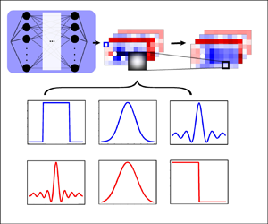
The classic physical isotropic spatial filters ($G$ in (3.1)) and its Fourier transformation in spectral space is shown in figure 4 (Cui, Xu & Zhang Reference Cui, Xu and Zhang2004). All filters satisfy the normalization condition to maintain the constants, and the kernel size of filters is represented as $\varDelta$. In this paper, all the experiments used the Gaussian kernel. The subsequent experiment verified that the FPDE results are not significantly affected by the type of filter. For details and results of the experiment, please refer to Appendix A.

Figure 4. The classic filters in physical and spectral space. The most common Gaussian weight filter kernel will be used in subsequent experiments.

In the context of the CV, the filter operation on data is usually called down sampling. When the filter is applied to the PDE calculation, it can be viewed as a new layer in the NN and builds the bridge between the ‘fully connected layer’ and ‘auto differentiation’ (shown in figure 5).

Figure 5. The physics-informed training framework and the proposed FPDE method. The example of solving the N–S equation governed problem. (a) The fully connected NN. A NN with multiple residual connections is used to model the observation. (b) The conventional PDE loss calculation process, which uses NN outputs in differentiation directly. (c) The improved framework in the PDE loss calculation iteration. The orange part is used to calculate the cross-terms in the equations and the green part is used to filter all variables. The PDEs are calculated with filtered variables instead. (d) The auto differentiation part. Derivatives are automatically generated from the computational graph.

The primary distinction between the regular model and the FPDE model is the calculation of the PDE. A multi-layer fully connected network is used as the body. The inputs of the NN are the coordinates $x$ and the time $t$. The unknown variables in the PDE are the NN outputs (N–S equations as an example in figure 5). In figure 5(b) the conventional process for calculating the PDE loss is depicted, wherein the differential terms are directly obtained from the NN outputs via auto differentiation. The improvements in the FPDE are shown in figure 5(c). In the orange box, the cross-terms in the N–S equations are calculated before the filter operation. The cross-terms are necessary since the filter operation does not satisfy the associative property of multiplication. Because of the filter operation, the product of two filtered variables is not equal to the filtered result of the product of two variables. The proposed filter, or the defined new activation layer, is shown in the green box. Benefiting from the mesh-free feature of the NN, the gridded outputs for the filter operation can be obtained. The $u$ is filtered to $\bar {u}$ by the Gaussian kernel, and the differential terms are calculated on the filtered outputs. Figure 5(d) is the calculation of equation constraints. Conventional PINN will use the original outputs to calculate the differential term, while the FPDE will use the filtered outputs. In calculating the residual form of the N–S equations, the Reynolds number of the training data, provided initially, is incorporated into the viscosity term.

In the training of the N–S equations case, a multi-layer NN with residual connections is used. The hidden layer of the NN has three paths with depths of 1, 4 and 16 blocks. The results of these three paths are summed before entering the output layer. Each block consists of a three-layer deep NN with 20 neurons per hidden layer and one residual connection (shown in the red box, figure 5a). The activation functions in this NN are all Swish functions.

The details of the training process for the FPDE and the conventional PDE model are summarized in table 1, which is a description of figure 5. Table 1 compares the difference between the FPDE and classical model more clearly. In both models, the form of the governing equations, initial and boundary conditions, and observation points are completely the same. The sole distinction lies in the FPDE intermediate layer between the forward propagation and auto differentiation parts, as depicted by the orange and green boxes in figure 5(b). In order to calculate the FPDE, the obtained NN inference outputs need to be gridded. The gridded outputs (i.e. $(\hat {u}_{col}, \hat {v}_{col}, \hat {p}_{col})$, 2-D case) are filtered by the given kernel at step 2.3. The filtered variables (i.e. $(\bar {u}_{col}, \bar {v}_{col}, \bar {p}_{col} )$) are pushed into the auto differentiation part to calculate the differential terms. In the whole FPDE process, the most critical steps are 2.2 and 2.3. Benefit from the meshless feature of the NN, velocity at any position can be obtained. Therefore, the filtering result can be calculated by obtaining the values of gridded neighbours of given points.

Table 1. The FPDE algorithm and comparison with the conventional algorithm.

In general, the calculation of FPDE loss can be divided into two steps: calculating cross-terms and filtering. The FPDE is transparent for NN architectures and forms of governing equations due to its simplicity. That means the FPDE can be applied to most NN architectures and different equations, not just the given example cases.

3.2. Theoretical improvements of filter

The FPDE method is deployed as the surrogate constraint of the original PDE loss. The FPDE constraint helps the optimization process of the NN and improves the model's performance in the ‘inference-filtering-optimization’ process. Owing to the intrinsic complexity of NNs, it is challenging to directly demonstrate the specific mechanisms through which the FPDE exerts its influence. In this section we aim to provide potential avenues of explanation and propose a putative mechanism that elucidates the underlying workings of the FPDE within the optimization framework of NNs.

3.2.1. Improvements in problems with the noisy data

Training with noisy data (like the restoration in figure 2b ii), the FPDE shows increased accuracy owing to the anti-noise ability of the filter operation. For the basic filter with the Gaussian kernel, the filtered output has a smaller variance than the original output, according to the Chebyshev's inequality (Saw, Yang & Mo Reference Saw, Yang and Mo1984). To illustrate this, we utilize normally distributed noise, $N(0, \sigma )$, which is a commonly used unbiased noise. After applying the filtering process, the FPDE utilizes data with reduced noise levels compared with the original, pre-filtered data. The procedure for calculating the PDE on noisy but filtered data is as follows:

(3.2)\begin{align} FPDE(\overline{\boldsymbol{y}+\boldsymbol{\epsilon}}) & = \frac{(\overline{u_i^{t+1} + \epsilon}) - (\overline{u_i^{t} + \epsilon})}{\Delta t} + \frac{\partial \overline{(u_i + \epsilon)(u_j + \epsilon)}}{\partial x_j} + \frac{1}{\rho} \frac{(\kern 1.5pt\overline{p^{x_i+1} + \epsilon}) - (\kern 1.5pt\overline{p^{x_i} + \epsilon})}{\Delta x_i}\nonumber\\ &\quad - \nu \frac{(\overline{u_i^{x_j+1} + \epsilon}) - 2(\overline{u_i^{x_j} + \epsilon}) + (\overline{u_i^{x_j-1} + \epsilon})}{\Delta x_j^2}, \end{align}

where $\epsilon$ and $\bar {\epsilon }$ represent the noise and filtered noise ($\epsilon \sim N(0, \sigma ), \bar {\epsilon } \sim N ( 0, {\sigma \sum \omega _i^2}/ {\sum ^2\omega _i} )$), $\omega _i$ represents the weight in filter ($\omega _i = ({1}/{\sqrt {2{\rm \pi} }})\exp (-{x^2}/{2})$). With the Gaussian kernel as the filter operator, the variance of noise decreases at the rate of $n^{-1}$ ($n$ is the size of the given Gaussian kernel). This indicates that just a small kernel can greatly reduce the interference of noise.

Observational data contaminated with noise can significantly diminish the precision of predictions generated by NNs. The effects and directional trends of such noise are illustrated in figure 6(a), where it is evident that data degradation progressively aligns the NN's output with the noisy dataset during each iterative cycle. This compromised output, subsequently influenced by the noise, can introduce bias into the computation of the PDEs.

Figure 6. Given possible mechanism of the FPDE method for processing noisy data. (a) Though the noisy data does not directly participate in the PDE loss calculation, it still affects the PDE loss by changing the NN output from the previous iteration. (b) The filtered NN outputs reduce the noise, making PDE calculations more robust and accurate.

Figure 6(b) presents a straightforward example, demonstrating that the output refined through a filtering process (represented by the blue star) more closely approximates the actual solution. This refined output point yields an accurate derivative, which is instrumental in mitigating the NN's susceptibility to noise. In contrast, outputs from a standard PDE model (depicted as blue dots) are subject to the distorting effects of noise (represented by the pink line), thereby failing to furnish the correct derivatives necessary for precise calculations.

In summary, the implementation of a filtering mechanism effectively diminishes the magnitude of noise interference. As a result, FPDEs are capable of yielding superior modelling outcomes even when the input data are noisy. It is hypothesized that the enhanced accuracy in the computation of differential terms is attributable to the reduced presence of noise within the filtered dataset.

3.2.2. Improvements in problems with the sparse data

In the context of sparse data problems, the enhancement brought by the FPDE can be viewed as an inverse application of the aforementioned mechanism. Within (3.2), the discrepancy in the optimization trajectory between the dataset and the PDE loss is mitigated through a filtering process. This intervention allows the NN to function without being impeded by the interplay of these two forms of loss. In § 2.1 it is hypothesized that the source of discord stems from the suboptimal quality of the input data. Empirical findings indicate that the FPDE approach persists in its optimization endeavours despite heightened conflict when training with sparse data. From a co-optimization perspective, the attenuation of this conflict can be interpreted as an inverse decoupling of the data and PDE loss elements.

In comparing the FPDE model with the conventional PDE model, particularly with respect to sparse data scenarios, the PDE loss takes a straightforward residual form that directly constrains the solution. Conversely, the FPDE model operates on the filtered ‘mean’ solution, as detailed in (3.3). Relative to the original problem, the FPDE-governed problem introduces additional variables that can be autonomously learned. When computing the equation's residual, the FPDE approach involves a greater number of NN inference outputs. Essentially, this allows for a broader spectrum of NN output values corresponding to the same filtered outcome, suggesting a richer set of potential solutions. From this vantage point, the FPDE effectively moderates the coupling between the PDE loss and data loss throughout the training process. The specific calculation formula is as follows:

(3.3)\begin{equation} \left.\begin{gathered} FPDE(\boldsymbol{\overline{y_{sparse}}}) =\frac{\overline{u_i^{T+1}} - \overline{u_i^{T}}}{\Delta T} + \frac{\partial \overline{u_i u_j}}{\partial X_j} + \frac{1}{\rho} \frac{\overline{p^{X_i+1}} - \overline{p^{X_i}}}{\Delta X_i} - \nu \frac{\overline{u_i^{X_j+1}} - 2\overline{u_i^{X_j}} + \overline{u_i^{X_j-1}}}{\Delta X_j^2} \\ \bar{u} = \frac{1}{\sum \omega_i} \sum_{i=1}^{n} \omega_i u_i, \quad \omega_i = \frac{1}{\sqrt{2{\rm \pi}}}\exp\left(-\frac{x^2}{2},\right) \end{gathered}\right\} \end{equation}

where $n$ is the filter size, the filtered variables are calculated from multiple NN outputs.

3.3. Design of experiments

Three experiments – the cylinder flow, cell migration and artery flow – are used to demonstrate the performance of the FPDE on sparse and noisy data. In the cylinder flow case, the improvements of the FPDE with simulation data are verified quantitatively; in the cell migration case, we evaluate the FPDE's ability to correct real data when equations have missing coefficients; in the arterial flow case, we assess the performance of the FPDE with inconsistent equations and observation data.

3.3.1. Simulation data of cylinder flow

To verify the improvement of the FPDE under sparse and noisy training data, the sparse dataset and noise dataset are designed for the quantitative experiment. In the experiment, the sampling ratio and noise level can be controlled to quantitatively demonstrate the improvement effect of the FPDE.

We designed two experiments to verify the FPDE improvements in sparsity and noise of training data. As shown in table 1, to generate sparse data for group 1, the datasets are randomly sampled using decreasing sampling ratios. To demonstrate the NN restoration ability under various levels of data missing, seven datasets of different sizes are employed in group 1. Obviously, the less observation it has, the more inaccuracy it produces. In group 2, noise is added to the $[u, v, p]$ field to make training more difficult (as demonstrated in proposition 2). The ‘additive white Gaussian noise’ (AWGN), the most common noise in the noise analysis, is chosen as the artificial noise added in $2^{-10}$ sampled dataset. The variances of the noise in $[u, v, p]$ are jointly decided by the standard deviation in $[u, v, p]$ and the noisy rate $r$ ($\epsilon _u = N(0, r {\cdot } std_u)$). Seven datasets of different noisy levels are used as the variables of group 2 to show the flow restoration ability with the different data error levels. As anticipated, higher levels of noise result in increased inaccuracies in the restoration process.

The entire simulation data are divided into three parts: the training, validation and test datasets. To test the restoration ability, the restoration outputs are plotted across the entire domain. The division is shown in figure 7.

Figure 7. The pre-possessing in full simulation data. In the experiments the training data are randomly sampled in the full dataset. In the sparse group the sampling ratio is the adjustable variable. In the noisy group the noisy level is the adjustable variable. Len is the total size of the dataset, and the sampling ratio indicates the proportion of training data to the dataset.

For details of cylinder flow, data sources and pre-processing methods, please refer to Appendix B. Figure 8 is an overview of the simulation data.

Figure 8. The numerical simulation data of the cylinder flow problem. The training data are sampled from the original data and contaminated with noise. Similar to the BC, the black circle is the cylinder wall.

Finally, experiments are conducted in two groups to evaluate the effects of sparsity and noise. The details of the two groups of datasets are presented in table 2. For each experiment, the FPDE and the baseline model are trained in parallel to show improvements. The processes of data sampling and adding noise are also described in Appendix B.

Table 2. Summary of two groups of data. These groups of data are used to train the FPDE and conventional PDE models and validate their flow restoration abilities under sparse and noisy conditions.

The evaluation criteria are defined in (3.4). The conventional PDE model and FPDE model are trained and tested on the same dataset. The evaluation criteria are defined as

(3.4)\begin{equation} \left.\begin{gathered} Loss = \frac{1}{N}\left|\left| \boldsymbol{y} - \boldsymbol{\hat{y}} \right|\right|_2 + \frac{1}{M}\left( \sum_{i=1}^{3} \left|\left| e_i \right|\right|_2 \right) + \frac{1}{W} \left|\left| \frac{\partial^k \boldsymbol{y}_{IC/BC}}{\partial \boldsymbol{x}^k_{IC/BC}} - \frac{\partial^k \boldsymbol{\hat{y}}_{IC/BC}}{\partial \boldsymbol{x}^k_{IC/BC}} \right|\right|, \\ e_1 = \frac{\partial u}{\partial t}+\left(u \frac{\partial u}{\partial x} + v \frac{\partial u}{\partial y}\right)+\frac{1}{\rho}\frac{\partial p}{\partial x} -\nu \left(\frac{\partial^2 u}{\partial x^2} + \frac{\partial^2 u}{\partial y^2}\right), \\ e_2 = \frac{\partial v}{\partial t}+\left(u \frac{\partial v}{\partial x} + v \frac{\partial v}{\partial y}\right)+\frac{1}{\rho}\frac{\partial p}{\partial y} -\nu \left(\frac{\partial^2 v}{\partial x^2} + \frac{\partial^2 v}{\partial y^2}\right), \\ e_3 = \frac{\partial u}{\partial x} + \frac{\partial v}{\partial y}, \end{gathered}\right\} \end{equation}

where $N,M,W$ represent the number of observations, collocation and IC/BC points in one iteration, respectively. Here $e_1,e_2,e_3$ represent the values of residual form PDE (N–S equations as an example); ${\partial ^k}/{\partial \boldsymbol {x}^k_{IC/BC}}$ represents the paradigm of BCs in different task (e.g. $k=0 / 1$ means the Dirichlet/Neumann BC).

3.3.2. Measurement data of cell migration

In this experiment, the real-world measurement data are used to demonstrate the improvement of the FPDE in real-world situations. Generally, there are two difficulties when using real data in this experiment. The first challenge stems from the high noise in the observation data. In the experiments, the measurement data are mainly obtained by sensors or manual measurements, which means the data are always noisy and sparse. When the measurement data are used as observation points in a physics-informed framework, it leads to conflict between data distribution and the theoretical equation. The cell number $C$ has high noise because the experimental data are automatically collected by the CV algorithm. The second challenge in this experiment is the missing coefficients in the equations. Since some coefficients of the equation are unknown, the NN predicts those segments without collocation points.

The cell migration data in reproducibility of scratch assays is affected by the initial cell density in the given scratch (Jin et al. Reference Jin, Shah, Penington, McCue, Chopin and Simpson2016). It shows the relationship of cell distribution in scratch assays with time, space and initial cell density. The data elucidates that when a scratch occurs, cells migrate to repair the scratch. Existing theories often use the Fisher–Kolmogorov model to describe the process of collective cell spreading, expressed as

(3.5)\begin{equation} \frac{\partial C}{\partial t} = D\frac{\partial^2 C}{\partial x^2} + \lambda C \left[ 1 - \frac{C}{K} \right], \end{equation}

where the dependent variable $C$ represents the cell concentration; $K$, $\lambda$ and $D$ represent the carrying capacity density, the cell diffusivity and the cell proliferation rate, respectively. In this context, $K$, $\lambda$ and $D$ can be viewed as the coefficients decided by initial cell density ($n$). Because this is a variable coefficient equation, it cannot calculate the unknown PDE at any collocation points. In the experiment described in this paper, the coefficients in $n=14\,000$ and $n=20\,000$ are known. The aim is to model the $n \in (14\,000, 20\,000)$ interval data through the FPDE training.

Figure 9 below is a schematic diagram of the cell migration experiment. For more details on the experiment, coefficients and dataset distribution, please refer to Appendix C.

Figure 9. The experiment of cell migration and data collection. (a) The square petri and counting method of blue lines. (b) Cells fill in the scratch by migrating. (c) Measurement data distribution.

In summary, the NN models the mapping relationship ‘$NN(t, x, n) \rightarrow C$’. When it comes to the calculation of the FPDE, the variable $C$ is filtered first and calculated in the same form as (3.6). Both the conventional PDE model and the FPDE model are trained until converged and tested on the same dataset. The final loss function in (2.1) can be written as

(3.6)\begin{equation} \left.\begin{gathered} Loss = \frac{1}{N}\left|\left| \boldsymbol{C} - \boldsymbol{\hat{C}} \right|\right|_2 + \frac{1}{M}\left(\left|\left| e \right|\right|_2 \right)\ + \frac{1}{W} \left|\left| \frac{\partial^k \boldsymbol{y}_{IC/BC}}{\partial \boldsymbol{x}^k_{IC/BC}} - \frac{\partial^k \boldsymbol{\hat y}_{IC/BC}}{\partial \boldsymbol{x}^k_{IC/BC}} \right|\right|, \\ e = \frac{\partial C}{\partial t} - 530.39\frac{\partial^2 C}{\partial x^2} - 0.066C + 46.42C^2 \quad {if} \ n=14\,000, \\ e = \frac{\partial C}{\partial t} - 982.26\frac{\partial^2 C}{\partial x^2} - 0.078C + 47.65C^2 \quad {if} \ n=20\,000, \\ e = 0 \quad {else}, \end{gathered}\right\} \end{equation}

where $N,M,W$ represent the number of observations, collocation and IC/BC points in one iteration, respectively; $e$ is the residual form value of (C1). Because of the changing coefficients, $e$ should be calculated according to three categories ($n=14\,000 / 20\,000/else$). The constants are obtained by regression in the experiment on Chen, Liu & Sun (Reference Chen, Liu and Sun2021b).

3.3.3. Measurement data of arterial flow

When the equation is obtained through the ideal model, there are always significant disparities between the actual situation and the description of the equation. In this experiment, arterial blood flow measurements are used to compare the modelling results of the FPDE and baseline with noisy data.

The data regarding arterial flow shows the velocity of blood when it flows through the arterial bifurcation (Kissas et al. Reference Kissas, Yang, Hwuang, Witschey, Detre and Perdikaris2020). The theoretical equations of velocity are shown as

(3.7)\begin{equation} \left.\begin{gathered} \frac{\partial A}{\partial t} ={-} \frac{\partial Au}{\partial x} , \quad \frac{\partial u}{\partial t} + u\frac{\partial u}{\partial x} ={-}\frac{1}{\rho}\frac{\partial p}{\partial x}, \\ A_1 u_1 = A_2 u_2 + A_3 u_3 , \quad p_1 + \frac{\rho}{2}u_1^2 = p_2 + \frac{\rho}{2}u_2^2 = p_3 + \frac{\rho}{2}u_3^2, \end{gathered}\right\} \end{equation}

where $A$ is the cross-sectional area of the vessel and $u$ is the axial velocity. Similar to the N–S equations (1.1, $\rho$ and $p$ represent density and pressure, respectively), $A_1$ and $u_1$ are the cross-sectional area and velocity of the interface in the aorta, $A_2, u_2$ and $A_3, u_3$ are the area and velocity of the interface in two bifurcations. The physical relationship between the aorta and two bifurcations is shown in figure 10(a), the real-world vessel's shape is shown in figure 10(b).

Figure 10. The experiment of one-dimensional blood flow in the $Y$-shaped artery. (a) The theoretical model (including the definitions of $A$, $A_i$ and $interface$). Equation (3.7) used in the training are derived from this model. (b) The location of five measurement points and the schematic diagram of the artery. (c) Overview of measurement data (area and velocity). (d) Multi-head NN to predict the velocity in different vessels.

An overview of the experiment is depicted in figure 10. Notably, a multi-head NN is used to fit different segments of vessels. Briefly, the aim is to train the NN with measurement data from only four observation points and model the entire blood vessel.

Figure 10 illustrates the experiment of one-dimensional blood flow in the Y-shaped artery. Previous studies modelled the velocity at the bifurcation based on an idealized Y-shaped one-dimensional vessel (shown in figure 10a). The actual blood is not ideal, thus, the measurement data can not always fit the embedding distribution in (3.7) well. The conflict raised in § 2.1 affects optimization a lot. In the real experiment measuring blood flow, the schematic diagram of an artery is shown in figure 10(b), with blood directions indicated by blue dotted lines. The data are measured at the five points, which are shown in figure 10(b), and the measured variables ($A, u$) are shown in figure 10(c). The in vivo data are measured by the magnetic resonance imaging (MRI) method in machine learning in cardiovascular flows modelling (Kissas et al. Reference Kissas, Yang, Hwuang, Witschey, Detre and Perdikaris2020). All data (area and velocity) are measured within 850 ms. Since the data are measured in an open vessel, the BC is unknown in training.

In order to model the distribution ‘$NN(t, x) \rightarrow (A, u, p)$’ in three parts of the vessel, we build a multi-head NN to predict the $(A, u, p)$ in different parts separately (shown in figure 10d). The NN is trained by the data from three endpoints (points 1, 2 and 3) and the interface (point 4). The collocation points are sampled among the entire vessel as constraints. The data in point 5 are reserved for testing. During parallel training, the baseline PDE is calculated directly. When calculating the FPDE, the variables $y = (A, u, p)$ are filtered first and calculated in the same form as in (3.8).

The conventional PDE model and FPDE model are trained until converged and tested in the same dataset. The final loss function in (2.1) can be written as

(3.8)\begin{equation} \left.\begin{gathered} Loss = \frac{1}{N}\left|\left| \boldsymbol{y} - \boldsymbol{\hat{y}} \right|\right|_2 + \frac{1}{M}\left( \sum_{i=1}^{2} \left|\left| e_i \right|\right|_2 \right) + \frac{1}{W}\left( \sum_{i=1}^{3} \left|\left| f_i \right|\right|_2 \right), \\ e_1 = \frac{\partial A}{\partial t} + \frac{\partial Au}{\partial x}, \quad e_2 = \frac{\partial u}{\partial t} + u\frac{\partial u}{\partial x} + \frac{1}{\rho}\frac{\partial p}{\partial x}, \\ f_1 = A_1 u_1 - A_2 u_2 - A_3 u_3, \\ f_2 = p_1 + \frac{\rho}{2}u_1^2 - p_2 - \frac{\rho}{2}u_2^2, \quad f_3 = p_1 + \frac{\rho}{2}u_1^2 - p_3 - \frac{\rho}{2}u_3^2, \end{gathered}\right\} \end{equation}

where $N,M,W$ represent the number of observations, collocation and interface points in one iteration, respectively; $e_1,e_2$ represent the residual value of governing equations, $f_1,f_2$ represent the residual value of the interface constraints that constrain mass and energy conservation in the interface.

4. Results

To ascertain the superiority of the FPDE constraint over the conventional PDE constraint, the performance of the corresponding models are compared in this section via multiple experiments. For comparison, the NN output, the residual map and the converged losses are plotted. The experimental findings offer evidence of the conflict – aligning with the hypotheses outlined in § 2.1) – and corroborate that the FPDE exhibits superior conflict resistance capabilities, a potential mechanism of which has been introduced in § 3.2).

4.1. The comparison between FPDE and baseline model

4.1.1. Quantitative analysis of simulation data

In the sparse data experiment, seven pairs of converged losses are shown in the histogram of figure 11(a). The simulation data are used as the ground truth in this experiment. The $x$ axis of this histogram is the number of simulation data used in the training dataset, and the bar on the $y$ axis is the MSE on the test data. The residuals between the ground truth and the NN restored flow field are plotted above the loss bar, where the top is the FPDE and below is the baseline residual. According to the colour map in the residual plot, a whiter colour means a solution that is closer to the ground truth. In figure 11(a) the residuals of the FPDE are generally less than those of the baseline. This improvement is consistent with the losses of histogram responses.

Figure 11. The NN outputs and MSE of the FPDE and baseline models. (a) The MSE and the residual between the ground truth and output. This result shows the FPDE method works better with sparse observation. (b) A typical example with a $2^{-16}$ sampling ratio. The comparisons of NN outputs ($u,v,p$) are below.

The FPDE model exhibits superior performance under sparse observation data, a common scenario in real-world applications. For example, under the $2^{-12}$ sampling ratio, the MSE of the converged FPDE model is only 18 % of the baseline. On average, the MSE on the converged FPDE model is 82.1 % less than the baseline model in these seven sparse cases. However, since the data in this experiment is accurate and the observation data of the first three groups are enough in quantity, the FPDE models show no improvements. In the magnified part in figure 11(a), the first three pairs of losses are close to the complete and error-free condition (i.e. case in figure 2c). Regarding the conflict, proposition 1 posits an assumption of nearly no conflict between the PDE and data loss. However, in the context of real-world measurements, data are invariably sparse, a scenario in which the FPDE models demonstrate enhanced performance.

Figure 11(b) shows the typical outputs in the sparse experiment. The restoration task is similar to the pure equations solving task at the lowest sampling ratio. Using the $2^{-16}$ sampling ratio case as the example, the number of used simulation data points is only 91. To show the sparsity directly, the comparison between the sampled data and full-size data points is shown on the top of figure 11(b). The direct NN outputs are shown for the comparison of two models. It is obvious that the PDE solution becomes more trivial (like the example in figure 3c). With the filter operation, the FPDE model can better capture the characteristic of the fluid.

In the noisy data experiment, the same kind of histogram and residuals are plotted in figure 12(a). The conflict with noisy data is shown as proposition 2, which is accurately reflected by the losses in the histogram. Under an identical noisy condition, the FPDE model always converged to a lower loss. Meanwhile, the residuals also show FPDE solutions are closer to the ground truth than the baseline model at all noise levels. Figure 12(b) is a typical example of this noisy group. At the highest noisy level (150 % standard deviation, additive white Gaussian noise), the generation of noisy data is shown on the top of figure 12(b). Under the high-noise condition, the large-scale features disappear, and periodicity is difficult to reflect. But the FPDE model still shows better anti-noise ability than the baseline model. Only by varying the physics-informed function can the FPDE model significantly reduce the impact of outliers. On average, the MSE on the FPDE model is 62.6 % less than the baseline model in these seven noisy cases. Under the high-noise data (noisy level >125 %), this number increases to 72.2 %.

Figure 12. The NN outputs and MSE of the FPDE and baseline models under the noisy data condition. (a) The MSE and residual plots. (b) The FPDE and PDE outputs under the additive white Gaussian noise with 150 % standard deviation of observation data; the comparison of NN outputs is below.

4.1.2. Experiment results of real-world data

The data in the cell migration case are sparse and noisy. Additionally, due to fluctuating coefficients, the NN lacks collocation points to learn the PDE on the test part. Both experimental results are shown in figure 13 (initial cell number, $n=16\,000/18\,000$). The predictions indicate the generalized ability of the NN to learn the embedding distribution from the given data. When confronted with an unknown equation, the NN learns the embedding physical process (i.e. the general law of cell migration) through generalization from given equations. In figure 13 the dots are the measurement data and the lines are the NN predictions. Quantitatively, the MSE of normalized prediction decreased from 0.157 (baseline) to 0.121 (FPDE), a decrease of 22.9 % when $n=16\,000$. When $n=18\,000$, this reduction increases to 42.9 %, from $9.89 \times 10^{-2}$ (baseline) to $5.64 \times 10^{-2}$ (FPDE).

Figure 13. Comparison in the cell migration test data ($\textrm {initial cell number} = [16\,000, 18\,000]$). Inside the red boxes, the difference between two outputs shows that the FPDE can overcome the influence of outliers better. This characteristic shows that the FPDE method has better modelling ability when faced with real, high-noise measurement data.

In the solutions of the baseline model, it is obvious that the high-noise initial data greatly affects the NN outputs. Outliers cause the NN to make predictions that contradict physical laws. Although both models predict worse outcomes over time (e.g. the red lines at $t=48$ h), the FPDE model still has more robust results. The unreasonable solution comes due to the inability of the outliers and the physical constraints to effectively correct the prediction well. In the comparison, the FPDE model gave better predictions in the test part. The filter operation mitigates the influence of outliers and makes theNN learn the embedding distribution successfully.

The difficulty in modelling the arterial flow data lies in the significant difference between the theoretical vessel model, which is used to derive the equations and real-world vessels. The NN prediction at point 5 is tested (shown in figure 10b) in the $Y$-shaped artery with measurement data. The comparison is shown in figure 14. As it demonstrated in the theoretical derivation in § 2.1, filter operations do not make the NN learn the small-scale fluctuations more finely, but they do make the NN model the large-scale information more precisely. On the large scale of the velocity field, the FPDE model is less inclined to produce trivial results compared with the baseline model. Despite the absence of pressure data in the measurements, the NN still gives a prediction of the pressure field through the physical constraints. Since the FPDE model is more accurate in the velocity field, it is intuitive that it has better prediction in the pressure field. Because the equations only constrain the $x$-direction derivative of pressure, figure 14 only shows the NN prediction of pressure individually.

Figure 14. Comparison in the arterial flow test data. The comparison of velocity and area at the test point is used to show the modelling ability of the FPDE and baseline models. Compared with the velocity field in the baseline model, the FPDE model learns better in large-scale fluctuations.

4.2. Existence of ‘conflict’ in loss analysis

In the motivation part (§ 2), we theoretically give the existence of conflict and how the conflict affects the co-optimization process. In our illustration, the conflict can be simply described as the ‘difference between the PDE and data loss optimization direction’. Therefore, we analyse the training losses and find the intuitive data evidence in figure 15.

Figure 15. Decoupling achieved by the FPDE method (reflected in training loss). (a) The PDE and data losses of two models until convergence. (b) The S and ‘exclusive OR’ colour bars. In order to show the distribution of the derivative sign, the colour bar is used in the after-pooling data of the original S. In the S plot, closer to red means more 0–1 oscillating and no effective gradient descent. In the $S_1 \oplus S_2$ plot, the blue colour indicates no conflict training process. Therefore, the effective descent in the baseline model only happened in the initial part, while the FPDE model realized decoupling throughout the whole training. (c) The definition and statistic result for each group of the conflict rate and conflict cost, which indicates higher conflict tolerance of the FPDE than the baseline.

The comparison between the FPDE model (up) and baseline model (down) is shown in figures 15(a) and 15(b). Figure 15(a) shows the equation loss and data loss of the FPDE and baseline model in the same experiment. In the baseline model the equation loss is the original PDE loss. Besides, the equation loss is the FPDE loss in the FPDE model. To analyse the correlation of the loss decreasing, we defined $S_1$ and $S_2$ as the sign of the equation and data loss derivative. To facilitate the following treatments, the Heaviside function is used to replace the sign operation. Thus, the losses are transferred to the 0/1 lists S, which show the increase or decrease in this iteration. But the 0/1 list is not straightforward, so we change it to a blue-red-blue colour bar for better demonstration. Specifically, we first average pool the original data of S and then map the after-pooling data to the blue-red-blue colour bar (the colour bar on the S left). Therefore, the S bars represent the randomness of loss as they change by colour. Because 0 and 1 represent the direction of loss change, the red colour in the middle of the colour bar indicates that there is oscillation in this section of the loss. Therefore, when S is in red, the training loss is oscillating, which means the optimization has no effective decrease. Conversely, when the colour of the S bar approaches blue, it means the training loss tends to steadily decrease or increase in this segment.

From the colour of the $S_1$ and $S_2$ bars, it is obvious that $S_1$ and $S_2$ of the baseline model in figure 15(b) are almost pure red. Meanwhile, the FPDE model still has many blue segments. This indicates that the baseline model is more unstable, whereas the FPDE model can optimize effectively.

The last two bars in figure 15(b) are the $S_1 \oplus S_2$ bar. Here $S_1$ and $S_2$ are used to show the directions of losses, thus, the $\oplus$ (exclusive OR, xor in short) can be used to show the consistency of $S_1$ and $S_2$. If $S_1$ and $S_2$ are inconsistent ($S_1 \oplus S_2=1$), that means there exists conflict in the co-optimization process. The $S_1 \oplus S_2$ bar is obtained by the exclusive OR solution of the $S_1$ and $S_2$ bars, where 1 means the direction between the equation and data loss is different and 0 means the same. After the pooling operation, the original data are also visualized with a red-white-blue colour bar, where red represents conflicts and blue represents the inverse.

The colour of the baseline model in $S_1 \oplus S_2$ shows the conflicts only exist during the initial fast decline segment, and the co-optimization is avoiding the potential conflict and trapping itself in the local optimum in the following segments. Meanwhile, the colour in the FPDE shows the stochastic conflicts that occurred, and the co-optimization does not pay much attention to the potential conflicts, which helps it find the global optimal. The calculation methods of conflict rate and conflict cost are as follows:

(4.1)\begin{align} \left.\begin{gathered} \text{Conflict rate } = \frac{1}{N}\sum S_1 \oplus S_2, \\ \text{Conflict cost } = \frac{1}{N}\sum \left.\left(\max\left(\frac{{\rm d}L_{data}}{{\rm d}L_{train}},\, \frac{{\rm d}L_{pde}}{{\rm d}L_{train}} \right)\right| S_1 \oplus S_2=1\right). \end{gathered}\right\} \end{align}

In figure 15(c), two statistical indicators are proposed to provide additional insights into the observations depicted in figure 15(b). The conflict rate is defined as the frequency of 1 in $S_1 \oplus S_2$ bar, and the conflict cost as the mean derivative of the increasing loss when the conflict happened (shown in (4.1)). These indicators are calculated on a group of losses with increasing noise and are plotted for general comparison. Though the two indicators exhibit an upward trend with escalating noise levels, the baseline model still prioritizes conflict avoidance in order to have a lower conflict rate and cost. The higher conflict in the FPDE reflects the decoupling process, which means the correlation between FPDE loss and data loss is decreased.

Overall, the results verify that the optimization process is effectively achieved by diminishing the correlation between the PDE and data loss. In the co-optimization process, the FPDE model can still optimize when facing higher conflict. These findings suggest that the FPDE model demonstrates greater effectiveness in addressing the challenges posed by noise and data sparsity commonly encountered in real-world measurement scenarios.

5. Conclusions

Since the data in real-world problems is often insufficient and noisy, it is necessary to improve the learning ability and robustness of the model. In other words, mitigating the reliance of the NN on data quality and quantity is a necessary prerequisite in the modelling of real-world data. One of the difficulties in the training of a physics-informed model is the conflict during the co-optimization. In this paper we analysed the causes of the conflict and proposed the FPDE method to overcome it. The improvement of the proposed FPDE is verified in three aspects: theoretical derivation, experiments on the simulation data and the experiments on real-world measurement data. In the comparison between the FPDE and baseline models, the proposed FPDE constraints have the following characteristics.

  1. (i) The FPDE is a general approach inspired by LES that applies to a variety of models, it is not designed for specific equations or NN architectures. As a surrogate constraint, it has good transferability in most cases.

  2. (ii) The FPDE method can help the NN model the noisy and sparse observation data better. This improvement is important for the practical applications of the physics-informed framework.

  3. (iii) The FPDE method can better optimize the NN when facing mismatches between the data and equations or the equation coefficients are missing.

Physics-informed methods have proliferated in recent years, and the FPDE surrogate constraint offers a notable reduction in the model's reliance on data quality and quantity. The proposed FPDE serves as a robust constraint for PINN, exhibiting superior performance in modelling real-world problems with sparse and noisy data, which is highly desirable in practical applications. Moreover, the utilization of the FPDE is straightforward, allowing for its application to other models by substituting the original equation constraints with filtered equations during the training process. This paper provides an explanation of the mechanism behind the improvement of the FPDE from a coupling perspective. The experimental results have shown that the FPDE loss is more prone to escaping local optima, as opposed to being tightly coupled with other losses. This decoupling mechanism not only facilitates easier optimization of the FPDE but also leads to improved results, especially in scenarios with sparse and highly noisy data. In future work, additional experiments will be conducted to explore the enhancements of filters in the context of NNs.

Funding

This work was supported by the National Natural Science Foundation of China (Grant No. 62106116), China Meteorological Administration under Grant QBZ202316, as well as by the High Performance Computing Centers at Eastern Institute of Technology, Ningbo, and Ningbo Institute of Digital Twin.

Declaration of interests

The authors report no conflict of interest.

Data availability statement

All codes used in this paper are publicly available on GitHub at https://github.com/Zzzz-Jonathan/FPDE. Additional data related to this paper may be requested from the authors.

Author contributions

D.Z., Y.C. and S.C. conceived the idea, designed the study and drafted the manuscript. D.Z. and Y.C. performed the coding, investigation and data analysis. Y.C. and S.C. modified and finalized the manuscript.

Appendix A. Influence of filter in FPDE

A.1. Filter type

In this experiment the FPDE models with different filters are trained with the same observation data. Thus, the accuracy of results is only determined by the type of filter. The observation data of cylinder flow with a 75 % standard deviation of noise are used. For comparison, the conventional physics-informed model is trained as the control group (i.e. no filter in figure 16). The MSEs of the results are shown in the figure below (figure 16).

Figure 16. The MSE of the FPDE models with different filters (including ‘no filter’). In this experiment the chosen classic filters are the box filter, the Gaussian filter and the low-pass filter. The conventional no-filter model is trained as the control group.

The results illustrate that all the given filters in the FPDE can improve the training result. Compared with the no-filter group, the improvements of different filters do not exhibit significant discrepancies. It is worth noting that due to the high computational cost of direct numerical simulation data, only one cylinder flow dataset is utilized in the experiment. This is a typical case used in many studies (e.g. Rao, Sun & Liu Reference Rao, Sun and Liu2020; Raissi et al. Reference Raissi, Yazdani and Karniadakis2020; Cheng et al. Reference Cheng, Meng, Li and Zhang2021), which facilitates comparisons between different studies. The results in Appendix A are specific to the cylinder flow studied in the experiments and may not be directly applicable to other scenarios.

A.2. Filter size

In the previous experiments, all results were based on the filter size ($\Delta x$) of 0.1. Therefore, this experiment is designed to examine the influence of filter size on FPDE results. Ideally, when the filter size is small enough, the FPDE result should converge to the conventional PINN result. In this experiment we used training data with a sampling ratio of $2^{-13}$ and $50\,\% \, std$ noise. The chosen filter is the Gaussian filter. In figure 17 we show the average MSE loss of the converged model on the test data over 10 repetitions.

Figure 17. The MSE of the FPDE models with different size Gaussian filters (including ‘no filter’). In this figure, $\Delta x$ is used to stand for the original filter of size 0.1.

The results roughly illustrate that the improvement of the FPDE will reach the optimum at an appropriate filter size. A filter size that is too large or too small will increase the MSE loss. It is worth noting that since the statistics on the results of different fluid cases is not enough, the above conclusions can only be roughly proven on the cylinder flow dataset of this work.

Appendix B. Details of cylinder flow

In this experiment the selected computation case is the 2-D cylinder flow (shown in § 1.1, the background information). The cylinder flow, governed by the N–S equation, is widely studied due to its intricate characteristics. Under the small-Reynolds-number (Re) condition, the fluid in the cylinder flow case shows the state of Stokes flow or creeping flow (Chilcott & Rallison Reference Chilcott and Rallison1988), which can be simply linearized to the solution of the steady N–S equation. The fluid becomes turbulent as $Re$ increases, and the velocity field shows periodicity. In the vorticity field the famous Kármán vortex street phenomenon appears (Wille Reference Wille1960).

The reference IC/BC conditions of the cylinder flow case are from the open resource data in the supplementary material of HFM (Raissi et al. Reference Raissi, Yazdani and Karniadakis2020), which is generated by OpenFOAM. These conditions are

(B1)\begin{equation} \left.\begin{gathered} u({-}10, y) = (1, 0), \\ u\left(\frac{1}{2}\cos\theta, \frac{1}{2}\sin\theta\right) = (0, 0), \quad \theta \in [0, 2{\rm \pi}], \end{gathered}\right\} \end{equation}

where zero pressure outflow and periodicity conditions are imposed in the boundary of $[-10, 30] {\cdot } [-10, 10]$ simulation domain, and the simulation data are selected in $[-2.5, 7.5] {\cdot } [-2.5, 2.5]$ area.

This simulation data satisfied the N–S equation, which is the ideal observation data in the condition written in proposition 1. In order to do the restoration in figure 2(b), two groups of experiments are designed to showcase the FPDE performances under varying levels of data quality and quantity. We assume that data quality and quantity can be summarized as its noise level and sparse level, thus, the simulation data of two groups is shown in table 1. To apply the control variate method, every case in each group has two parallel models. The only difference between two parallel models is the constraint imposed on the PDE or FPDE loss. The conventional PDE guided model is used as the baseline model for this question, using the same data in both models during each pair of experiments. In order to balance the additional computational cost caused by filter operation in the FPDE model, the batch size of the baseline model is scaled up k times (where k denotes the filter size). Each model is trained for 50 000 iterations and tested in the whole selected domain ($x \in [-2.5, 7.5]$, $y \in [-2.5, 2.5]$ and $t \in [0, 16]$). Thus, the comparison reflects the improvement of the FPDE constraint compared with the conventional PDE constraint.

The training process terminates when the training loss has converged. The final loss function in (2.1) can be written as (3.4). When training the FPDE model, the variables $y = (u, v, p)$ are filtered initially and are subsequently calculated in the same form as (3.4). Each L2 error in the training process is recorded for analysis. The NN parameters are saved every 100 iterations and during iterations where the smallest validation loss is achieved.

Appendix C. Details of cell migration

In (3.5) the constants $D$, $\lambda$ and $K$ are always obtained by regression. In the experiments, these constants can be obtained by the ordinary least squares method with measurement data. Furthermore, the simplified equations are obtained in the knowledge discovery field in (C1) (Chen et al. Reference Chen, Liu and Sun2021b):

(C1)\begin{equation} \left.\begin{gathered} \frac{\partial C}{\partial t} = 530.39\frac{\partial^2 C}{\partial x^2} + 0.066C - 46.42C^2, \quad n=14\,000, \\ \frac{\partial C}{\partial t} = 982.26\frac{\partial^2 C}{\partial x^2} + 0.078C - 47.65C^2, \quad n=20\,000. \end{gathered}\right\} \end{equation}

Here $n$ is the initial cell number. In this equation the coefficients $D, \lambda, K$ are decided by initial cell number ($n$), which means the initial density of the cell can effect the scratch recover process.

The measurement data are generated by the cell migration experiment in square petri dishes. Over time, cells migrate and gradually fill in a scratch within the dishes, with cell densities between demarcated blue lines being quantified at 12-hour intervals. Four parallel experiments with different initial cell numbers ($n=14\,000/16\,000/18\,000/20\,000$) are measured to show the effect of $n$ on cell density. The example of actual measured data is shown in figure 9(c), where the $y$ axis represents the cell density between adjacent blue lines ($\textrm {cells}\ \mathrm {\mu } \textrm {m}^{-2}$) and the $x$ axis is the location ($\mathrm {\mu } \textrm {m}$). The density data in $t=0$ is used as the initial data, while subsequent data points ($t=12\ \textrm {h}/24\ \textrm {h}/36\ \textrm {h}/48\ \textrm {h}$) are those that the NN is tasked with predicting.

When collecting data for the experiments the measurement data exhibits a high level of noise and conducting replicative experiments is prohibitively expensive. Moreover, the data are so sparse in the dimension of n (cell number) that it is impossible to find all coefficients for each n. In terms of the NN training, it is particularly important that the collocation points can not be selected randomly because of the unknown coefficients. Thus, it only has the collocation points in $n=14\,000$ and 20 000 flat to calculate (C1). The task is modelling the distribution of unknown equations ($n \in (14\,000, 20\,000)$) by the conventional PDE/FPDE method. The training data distribution is shown in figure 18.

Figure 18. The training data in cell migration modelling. The dataset's initial cell numbers are 14 000 and 20 000 for the NN training. Depending on the initial cell number, different groups fill the scratch at different speeds.

References

Cai, S., Wang, Z., Fuest, F., Jeon, Y.J., Gray, C. & Karniadakis, G.Em. 2021 a Flow over an espresso cup: inferring 3-D velocity and pressure fields from tomographic background oriented Schlieren via physics-informed neural networks. J. Fluid Mech. 915, A102.CrossRefGoogle Scholar
Cai, S., Wang, Z., Wang, S., Perdikaris, P. & Karniadakis, G.Em. 2021 b Physics-informed neural networks for heat transfer problems. Trans. ASME J. Heat Transfer 143 (6), 060801.CrossRefGoogle Scholar
Chen, F., Sondak, D., Protopapas, P., Mattheakis, M., Liu, S., Agarwal, D. & Di Giovanni, M. 2020 Neurodiffeq: a python package for solving differential equations with neural networks. J. Open Source Softw. 5 (46), 1931.CrossRefGoogle Scholar
Chen, Y., Huang, D., Zhang, D., Zeng, J., Wang, N., Zhang, H. & Yan, J. 2021 a Theory-guided hard constraint projection (HCP): a knowledge-based data-driven scientific machine learning method. J. Comput. Phys. 445, 110624.CrossRefGoogle Scholar
Chen, Y., Luo, Y., Liu, Q., Xu, H. & Zhang, D. 2022 Symbolic genetic algorithm for discovering open-form partial differential equations (SGA-PDE). Phys. Rev. Res. 4 (2), 023174.CrossRefGoogle Scholar
Chen, Y. & Zhang, D. 2022 Integration of knowledge and data in machine learning. arXiv:2202.10337.Google Scholar
Chen, Z., Liu, Y. & Sun, H. 2021 b Physics-informed learning of governing equations from scarce data. Nat. Commun. 12 (1), 113.Google ScholarPubMed
Cheng, C., Meng, H., Li, Y.-Z. & Zhang, G.-T. 2021 Deep learning based on pinn for solving 2 DOF vortex induced vibration of cylinder. Ocean Engng 240, 109932.CrossRefGoogle Scholar
Chilcott, M.D. & Rallison, J.M. 1988 Creeping flow of dilute polymer solutions past cylinders and spheres. J. Non-Newtonian Fluid Mech. 29, 381432.CrossRefGoogle Scholar
Clark Di Leoni, P., Agarwal, K., Zaki, T.A., Meneveau, C. & Katz, J. 2023 Reconstructing turbulent velocity and pressure fields from under-resolved noisy particle tracks using physics-informed neural networks. Exp. Fluids 64 (5), 95.CrossRefGoogle Scholar
Cui, G.X., Xu, C.X. & Zhang, Z.S. 2004 Progress in large eddy simulation of turbulent flows. Acta Aerodyn. Sin. 22 (2), 121129.Google Scholar
Cuomo, S., Di Cola, V.S., Giampaolo, F., Rozza, G., Raissi, M. & Piccialli, F. 2022 Scientific machine learning through physics–informed neural networks: where we are and what's next. J. Sci. Comput. 92 (3), 88.CrossRefGoogle Scholar
DebRoy, T., Mukherjee, T., Wei, H.L., Elmer, J.W. & Milewski, J.O. 2021 Metallurgy, mechanistic models and machine learning in metal printing. Nat. Rev. Mater. 6 (1), 4868.CrossRefGoogle Scholar
Du, M., Chen, Y. & Zhang, D. 2022 AutoKE: an automatic knowledge embedding framework for scientific machine learning. IEEE Trans. Artif. Intell. 4 (6), 1564–1578.Google Scholar
Du, Y., Wang, M. & Zaki, T.A. 2023 State estimation in minimal turbulent channel flow: a comparative study of 4DVar and PINN. Intl J. Heat Fluid Flow 99, 109073.CrossRefGoogle Scholar
Duraisamy, K. 2021 Perspectives on machine learning-augmented Reynolds-averaged and large eddy simulation models of turbulence. Phys. Rev. Fluids 6 (5), 050504.CrossRefGoogle Scholar
Duraisamy, K., Iaccarino, G. & Xiao, H. 2019 Turbulence modeling in the age of data. Annu. Rev. Fluid Mech. 51, 357377.CrossRefGoogle Scholar
Fukushima, K. & Miyake, S. 1982 Neocognitron: a self-organizing neural network model for a mechanism of visual pattern recognition. In Competition and Cooperation in Neural Nets, pp. 267–285. Springer.CrossRefGoogle Scholar
Glowinski, R. & Pironneau, O. 1992 Finite element methods for Navier–Stokes equations. Annu. Rev. Fluid Mech. 24 (1), 167204.CrossRefGoogle Scholar
Goodell, J.W., Kumar, S., Lim, W.M. & Pattnaik, D. 2021 Artificial intelligence and machine learning in finance: identifying foundations, themes, and research clusters from bibliometric analysis. J. Behav. Exp. Fin. 32, 100577.CrossRefGoogle Scholar
Goodfellow, I.J., Vinyals, O. & Saxe, A.M. 2014 Qualitatively characterizing neural network optimization problems. arXiv:1412.6544.Google Scholar
Goswami, S., Anitescu, C., Chakraborty, S. & Rabczuk, T. 2020 Transfer learning enhanced physics informed neural network for phase-field modeling of fracture. Theor. Appl. Fract. Mech. 106, 102447.CrossRefGoogle Scholar
Hartman, E.J., Keeler, J.D. & Kowalski, J.M. 1990 Layered neural networks with Gaussian hidden units as universal approximations. Neural Comput. 2 (2), 210215.CrossRefGoogle Scholar
Hasanuzzaman, G., Eivazi, H., Merbold, S., Egbers, C. & Vinuesa, R. 2023 Enhancement of PIV measurements via physics-informed neural networks. Meas. Sci. Technol. 34 (4), 044002.CrossRefGoogle Scholar
Jin, W., Shah, E.T., Penington, C.J., McCue, S.W., Chopin, L.K. & Simpson, M.J. 2016 Reproducibility of scratch assays is affected by the initial degree of confluence: experiments, modelling and model selection. J. Theor. Biol. 390, 136145.CrossRefGoogle ScholarPubMed
Kissas, G., Yang, Y., Hwuang, E., Witschey, W.R., Detre, J.A. & Perdikaris, P. 2020 Machine learning in cardiovascular flows modeling: predicting arterial blood pressure from non-invasive 4D flow MRI data using physics-informed neural networks. Comput. Meth. Appl. Mech. Engng 358, 112623.CrossRefGoogle Scholar
Li, T., Buzzicotti, M., Biferale, L., Bonaccorso, F., Chen, S. & Wan, M. 2022 Data reconstruction of turbulent flows with gappy POD, extended POD and generative adversarial networks. arXiv:2210.11921.Google Scholar
Li, Z., Kovachki, N., Azizzadenesheli, K., Liu, B., Bhattacharya, K., Stuart, A. & Anandkumar, A. 2020 Fourier neural operator for parametric partial differential equations. arXiv:2010.08895.Google Scholar
Littmann, M. et al. 2020 Validity of machine learning in biology and medicine increased through collaborations across fields of expertise. Nat. Mach. Intell. 2 (1), 1824.CrossRefGoogle Scholar
Lu, L., Meng, X., Mao, Z. & Karniadakis, G.Em. 2021 DeepXDE: a deep learning library for solving differential equations. SIAM Rev. 63 (1), 208228.CrossRefGoogle Scholar
Maulik, R., San, O., Rasheed, A. & Vedula, P. 2019 Subgrid modelling for two-dimensional turbulence using neural networks. J. Fluid Mech. 858, 122144.CrossRefGoogle Scholar
Misyris, G.S., Venzke, A. & Chatzivasileiadis, S. 2020 Physics-informed neural networks for power systems. In 2020 IEEE Power & Energy Society General Meeting (PESGM), pp. 1–5. IEEE.CrossRefGoogle Scholar
Piomelli, U. 1999 Large-eddy simulation: achievements and challenges. Prog. Aerosp. Sci. 35 (4), 335362.CrossRefGoogle Scholar
Raissi, M., Perdikaris, P. & Karniadakis, G.E. 2019 Physics-informed neural networks: a deep learning framework for solving forward and inverse problems involving nonlinear partial differential equations. J. Comput. Phys. 378, 686707.CrossRefGoogle Scholar
Raissi, M., Yazdani, A. & Karniadakis, G.Em. 2020 Hidden fluid mechanics: learning velocity and pressure fields from flow visualizations. Science 367 (6481), 10261030.CrossRefGoogle ScholarPubMed
Rao, C., Sun, H. & Liu, Y. 2020 Physics-informed deep learning for incompressible laminar flows. Theor. Appl. Mech. Lett. 10 (3), 207212.CrossRefGoogle Scholar
Rasheed, A., San, O. & Kvamsdal, T. 2020 Digital twin: values, challenges and enablers from a modeling perspective. IEEE Access 8, 2198022012.CrossRefGoogle Scholar
Rong, M., Zhang, D. & Wang, N. 2022 A Lagrangian dual-based theory-guided deep neural network. Complex Intell. Syst. 8 (6), 48494862.CrossRefGoogle Scholar
Ruder, S. 2016 An overview of gradient descent optimization algorithms. arXiv:1609.04747.Google Scholar
Rudy, S.H., Brunton, S.L., Proctor, J.L. & Kutz, J.N. 2017 Data-driven discovery of partial differential equations. Sci. Adv. 3 (4), e1602614.CrossRefGoogle ScholarPubMed
Sag, I.A., Baldwin, T., Bond, F., Copestake, A. & Flickinger, D. 2002 Multiword expressions: a pain in the neck for NLP. In International Conference on Intelligent Text Processing and Computational Linguistics, pp. 1–15. Springer.CrossRefGoogle Scholar
Saw, J.G., Yang, M.C.K. & Mo, T.C. 1984 Chebyshev inequality with estimated mean and variance. Am. Stat. 38 (2), 130132.CrossRefGoogle Scholar
Schäfer, M., Turek, S., Durst, F., Krause, E. & Rannacher, R. 1996 Benchmark computations of laminar flow around a cylinder. In Flow Simulation with High-Performance Computers II, pp. 547–566. Springer.CrossRefGoogle Scholar
Shukla, K., Di Leoni, P.C., Blackshire, J., Sparkman, D. & Karniadakis, G.Em. 2020 Physics-informed neural network for ultrasound nondestructive quantification of surface breaking cracks. J. Nondestruct. Eval. 39 (3), 120.CrossRefGoogle Scholar
Smagorinsky, J. 1963 General circulation experiments with the primitive equations: I. The basic experiment. Mon. Weath. Rev. 91 (3), 99164.2.3.CO;2>CrossRefGoogle Scholar
Temam, R. 1995 Navier–Stokes Equations and Nonlinear Functional Analysis. SIAM.CrossRefGoogle Scholar
Vernon, D. 1991 Machine Vision: Automated Visual Inspection and Robot Vision. Prentice-Hall, Inc.Google Scholar
Wang, C.Y. 1991 Exact solutions of the steady-state Navier–Stokes equations. Annu. Rev. Fluid Mech. 23 (1), 159177.CrossRefGoogle Scholar
Wang, C., Bentivegna, E., Zhou, W., Klein, L. & Elmegreen, B. 2020 a Physics-informed neural network super resolution for advection-diffusion models. arXiv:2011.02519.Google Scholar
Wang, C. & Peng, K. 2023 AI experience predicts identification with humankind. Behav. Sci. 13 (2), 89.CrossRefGoogle ScholarPubMed
Wang, H., Liu, Y. & Wang, S. 2022 a Dense velocity reconstruction from particle image velocimetry/particle tracking velocimetry using a physics-informed neural network. Phys. Fluids 34 (1), 017116.Google Scholar
Wang, N., Zhang, D., Chang, H. & Li, H. 2020 b Deep learning of subsurface flow via theory-guided neural network. J. Hydrol. 584, 124700.CrossRefGoogle Scholar
Wang, S., Teng, Y. & Perdikaris, P. 2021 Understanding and mitigating gradient flow pathologies in physics-informed neural networks. SIAM J. Sci. Comput. 43 (5), A3055A3081.CrossRefGoogle Scholar
Wang, S., Yu, X. & Perdikaris, P. 2022 b When and why PINNs fail to train: a neural tangent kernel perspective. J. Comput. Phys. 449, 110768.CrossRefGoogle Scholar
Wille, R. 1960 Kármán vortex streets. Adv. Appl. Mech. 6, 273287.CrossRefGoogle Scholar
Xu, H., Chang, H. & Zhang, D. 2019 DL-PDE: deep-learning based data-driven discovery of partial differential equations from discrete and noisy data. arXiv:1908.04463.Google Scholar
Yuan, Z., Xie, C. & Wang, J. 2020 Deconvolutional artificial neural network models for large eddy simulation of turbulence. Phys. Fluids 32 (11), 115106.CrossRefGoogle Scholar
Zhang, H., Goodfellow, I., Metaxas, D. & Odena, A. 2019 Self-attention generative adversarial networks. In International Conference on Machine Learning, pp. 7354–7363. PMLR.Google Scholar
Zhou, K., Li, J., Hong, J. & Grauer, S.J. 2023 Stochastic particle advection velocimetry (SPAV): theory, simulations, and proof-of-concept experiments. Meas. Sci. Technol. 34 (6), 065302.CrossRefGoogle Scholar
Figure 0

Figure 1. The fluid flow through a cylinder wall (streak lines). To keep the consistency of data, the reference simulation solutions are from the open resource data of hidden fluid mechanics (Raissi, Yazdani & Karniadakis 2020).

Figure 1

Figure 2. Summary of the physics-informed training tasks. (a) The extrapolation, where known and unknown parts conform to the different data distributions. The NN is trained to learn the hidden pattern in the known part and extrapolate it in the unknown part. (b) The restoration, of which the given and unknown parts conform to the same data distribution. Meanwhile, the data has poor quality and quantity. Panel (b i) shows the restoration from sparse data and (b ii) is the restoration from noisy data. (c) Sufficient and accurate data with the same distribution, which makes the task an ordinary interpolation problem.

Figure 2

Figure 3. The NN output guided by different equations. (a) The Burgers equation is the classic example in PINN (Raissi et al.2019), which is used to show the effect of regularity. (b) The exponential function, which shows the difficulty of the NN to handle the interval with a small loss value. The NN always focuses on the large loss interval. (c) The N–S equation. Facing the complex solution, the NN tends to be trapped in the local minimum and obtain the trivial solution.

Figure 3

Figure 4. The classic filters in physical and spectral space. The most common Gaussian weight filter kernel will be used in subsequent experiments.

Figure 4

Figure 5. The physics-informed training framework and the proposed FPDE method. The example of solving the N–S equation governed problem. (a) The fully connected NN. A NN with multiple residual connections is used to model the observation. (b) The conventional PDE loss calculation process, which uses NN outputs in differentiation directly. (c) The improved framework in the PDE loss calculation iteration. The orange part is used to calculate the cross-terms in the equations and the green part is used to filter all variables. The PDEs are calculated with filtered variables instead. (d) The auto differentiation part. Derivatives are automatically generated from the computational graph.

Figure 5

Table 1. The FPDE algorithm and comparison with the conventional algorithm.

Figure 6

Figure 6. Given possible mechanism of the FPDE method for processing noisy data. (a) Though the noisy data does not directly participate in the PDE loss calculation, it still affects the PDE loss by changing the NN output from the previous iteration. (b) The filtered NN outputs reduce the noise, making PDE calculations more robust and accurate.

Figure 7

Figure 7. The pre-possessing in full simulation data. In the experiments the training data are randomly sampled in the full dataset. In the sparse group the sampling ratio is the adjustable variable. In the noisy group the noisy level is the adjustable variable. Len is the total size of the dataset, and the sampling ratio indicates the proportion of training data to the dataset.

Figure 8

Figure 8. The numerical simulation data of the cylinder flow problem. The training data are sampled from the original data and contaminated with noise. Similar to the BC, the black circle is the cylinder wall.

Figure 9

Table 2. Summary of two groups of data. These groups of data are used to train the FPDE and conventional PDE models and validate their flow restoration abilities under sparse and noisy conditions.

Figure 10

Figure 9. The experiment of cell migration and data collection. (a) The square petri and counting method of blue lines. (b) Cells fill in the scratch by migrating. (c) Measurement data distribution.

Figure 11

Figure 10. The experiment of one-dimensional blood flow in the $Y$-shaped artery. (a) The theoretical model (including the definitions of $A$, $A_i$ and $interface$). Equation (3.7) used in the training are derived from this model. (b) The location of five measurement points and the schematic diagram of the artery. (c) Overview of measurement data (area and velocity). (d) Multi-head NN to predict the velocity in different vessels.

Figure 12

Figure 11. The NN outputs and MSE of the FPDE and baseline models. (a) The MSE and the residual between the ground truth and output. This result shows the FPDE method works better with sparse observation. (b) A typical example with a $2^{-16}$ sampling ratio. The comparisons of NN outputs ($u,v,p$) are below.

Figure 13

Figure 12. The NN outputs and MSE of the FPDE and baseline models under the noisy data condition. (a) The MSE and residual plots. (b) The FPDE and PDE outputs under the additive white Gaussian noise with 150 % standard deviation of observation data; the comparison of NN outputs is below.

Figure 14

Figure 13. Comparison in the cell migration test data ($\textrm {initial cell number} = [16\,000, 18\,000]$). Inside the red boxes, the difference between two outputs shows that the FPDE can overcome the influence of outliers better. This characteristic shows that the FPDE method has better modelling ability when faced with real, high-noise measurement data.

Figure 15

Figure 14. Comparison in the arterial flow test data. The comparison of velocity and area at the test point is used to show the modelling ability of the FPDE and baseline models. Compared with the velocity field in the baseline model, the FPDE model learns better in large-scale fluctuations.

Figure 16

Figure 15. Decoupling achieved by the FPDE method (reflected in training loss). (a) The PDE and data losses of two models until convergence. (b) The S and ‘exclusive OR’ colour bars. In order to show the distribution of the derivative sign, the colour bar is used in the after-pooling data of the original S. In the S plot, closer to red means more 0–1 oscillating and no effective gradient descent. In the $S_1 \oplus S_2$ plot, the blue colour indicates no conflict training process. Therefore, the effective descent in the baseline model only happened in the initial part, while the FPDE model realized decoupling throughout the whole training. (c) The definition and statistic result for each group of the conflict rate and conflict cost, which indicates higher conflict tolerance of the FPDE than the baseline.

Figure 17

Figure 16. The MSE of the FPDE models with different filters (including ‘no filter’). In this experiment the chosen classic filters are the box filter, the Gaussian filter and the low-pass filter. The conventional no-filter model is trained as the control group.

Figure 18

Figure 17. The MSE of the FPDE models with different size Gaussian filters (including ‘no filter’). In this figure, $\Delta x$ is used to stand for the original filter of size 0.1.

Figure 19

Figure 18. The training data in cell migration modelling. The dataset's initial cell numbers are 14 000 and 20 000 for the NN training. Depending on the initial cell number, different groups fill the scratch at different speeds.