


1. Introduction
The present study is motivated by the problem of heat and mass transfer across the air–water surfaces of natural water bodies. An example of this is the transfer of heat and atmospheric gases (such as oxygen, carbon dioxide, methane) across the water surface in lakes and reservoirs. An accurate prediction of the transfer rate is important in order to produce a reliable global heat and greenhouse gas budget. Typically, wind shear is seen as the main source of turbulence generation that promotes interfacial heat and mass flux (Wanninkhof et al. Reference Wanninkhof, Asher, Ho and Sweeney2009; Garbe et al. Reference Garbe2014). Other turbulence sources, especially buoyancy, are thereby usually neglected. Recently, buoyancy-driven heat and gas transfer induced by surface cooling, which is particularly important in lakes and ponds at low wind speeds, has attracted increasing attention (Rutgersson & Smedman Reference Rutgersson and Smedman2010; Podgrajsek, Sahlee & Rutgersson Reference Podgrajsek, Sahlee and Rutgersson2014; MacIntyre et al. Reference MacIntyre, Crowe, Cortés and Arneborg2018). In this process, due to surface cooling (usually by evaporation), plumes and sheets of relatively heavy, cold (gas-saturated) surface water plunge down and are replaced by warm (unsaturated) bulk water, thereby promoting heat and gas transfer across the surface.
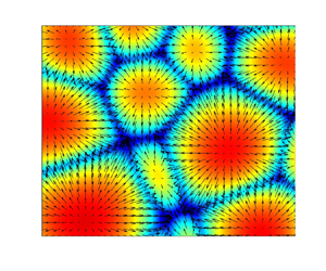
It is known that surface cooling not only results in unstable density gradients, but also may induce variation in surface tension due to local changes in surface temperature. Such variations in surface tension generate so-called Marangoni forces that induce flows from low-surface-tension (high-temperature) regions to high-surface-tension (low-temperature) regions. As a result of the buoyancy-induced and/or Marangoni-induced convective instabilities, convection cells are generated at the surface (e.g. Spangenberg & Rowland Reference Spangenberg and Rowland1961; Maroto, Pérez-Muñuzuri & Romero-Cano Reference Maroto, Pérez-Muñuzuri and Romero-Cano2007). The typical footprint of these convection cells indicates the presence of one or more high-temperature regions in their interior (Wissink & Herlina Reference Wissink and Herlina2016), and shows that individual cells are separated by narrow regions of low temperature. Various theoretical and experimental studies have been carried out to investigate the onset of the underlying instability and the resulting pattern formation (see e.g. Pearson Reference Pearson1958; Chandrasekhar Reference Chandrasekhar1961; Bodenschatz, Pesch & Ahlers Reference Bodenschatz, Pesch and Ahlers2000; Nepomnyashchy, Legros & Simanovskii Reference Nepomnyashchy, Legros and Simanovskii2006).
Most of these studies were motivated by chemical engineering applications, and employed a relatively thin layer of fluid bounded from below by a solid wall (no-slip boundary). These studies showed that in a thin layer of fluid such horizontal temperature-gradient-induced Marangoni forces act together with buoyancy forces to promote mixing of cool surface water with warmer water from the (upper) bulk (e.g. Nield Reference Nield1964; Toussaint et al. Reference Toussaint, Bodiguel, Doumenc, Guerrier and Allain2008).
Studies of this convective instability in non-shallow water bodies with a free surface, such as the work carried out by Spangenberg & Rowland (Reference Spangenberg and Rowland1961), Davenport (Reference Davenport1972), Tan & Thorpe (Reference Tan and Thorpe1996) and Flack, Saylor & Smith (Reference Flack, Saylor and Smith2001), are relatively few. Tan & Thorpe (Reference Tan and Thorpe1996) reported that surface-tension-driven convection usually only dominates in relatively thin layers of fluid (up to about  $4$ mm in thickness), while for layers thicker than
  $10$ mm (as usually encountered in environmental engineering problems) buoyancy-driven convection dominates. The former would imply that, especially in a developing convective instability, Marangoni forces cannot be ignored as the maximum thickness of the thermal boundary layer (which is the most relevant thermal length scale) tends to be much smaller than
  $4$ mm, irrespective of the water depth.
In previous three-dimensional unsteady numerical simulations of buoyancy-driven heat transfer across the air–water surface in relatively deep bodies of water, the physical effect of surface cooling was modelled by prescribing either a constant temperature (Wissink & Herlina Reference Wissink and Herlina2016) or a constant heat flux (Handler et al. Reference Handler, Saylor, Leighton and Rovelstad1999; Fredriksson et al. Reference Fredriksson, Arneborg, Nilsson, Zhang and Handler2016). In contrast to simulations with a constant surface temperature, in constant-heat-flux simulations variations in surface temperature typically occur which generate Marangoni forces. Despite their potentially significant contribution to the heat and mass transfer coefficients, these forces were usually ignored.
It should be noted that Marangoni forces can also be generated by local concentration variations of a component in a multicomponent fluid. An example of this can be found in evaporating binary droplets that contain water mixed with another fluid of different volatility and density. Here, evaporation of the more volatile component induces density differences as well as surface tension gradients. As a result, a competition between buoyant and Marangoni convection is obtained causing a variety of convection patterns (see Diddens, Li & Lohse (Reference Diddens, Li and Lohse2021) and references therein). Another example are the surfactant-concentration-induced Marangoni forces studied by, for example, Khakpour, Shen & Yue (Reference Khakpour, Shen and Yue2011) and Wissink et al. (Reference Wissink, Herlina, Akar and Uhlmann2017). In the latter study, a wide range of contamination levels was considered. It was shown that the interfacial mass transfer reduces monotonically with surfactant concentration, and a model was derived that predicts the interfacial mass transfer from a snapshot of the surfactant concentration distribution and turbulent flow characteristics of the water.
While surfactant-concentration-induced Marangoni forces were found to significantly reduce near-surface turbulence (and hence interfacial heat and mass transfer), the effect of the surface-temperature-gradient-induced Marangoni forces (studied here) would be to enhance the near-surface convection, thereby working in accord with the buoyant instability. To carry out a detailed investigation of the importance of Marangoni forces and their interaction with buoyancy forces in the initial development of the Rayleigh–Bénard–Marangoni (RBM) instability, fully resolved, three-dimensional, time-accurate numerical simulations were performed. In the simulations, evaporative cooling was modelled by a constant heat flux. Care was taken to ensure that the depth of the computational domain was sufficient to accurately represent the early stages of the development of the RBM instability in a deep body of water. The size of the computational domain as well as the interfacial heat flux were chosen in accordance with the typical set-up of laboratory experiments, such as those of Foster (Reference Foster1965). Direct numerical simulations (DNS) were performed for a wide range of Rayleigh ( $Ra_L$) and Marangoni (
 $Ma_L$) numbers, including cases with
  $Ra_L=0$ and
  $Ma_L=0$, representing purely surface-tension-driven convection and purely buoyancy-driven convection, respectively.
2. Computational aspects
As mentioned above, this study is motivated by the problem of heat transfer across a water surface. In the range of temperatures considered, the water density varies approximately linearly with temperature. Because of the very small changes in density, the Boussinesq approximation is used to describe the flow induced by the unstable stratification near the surface. The non-dimensional Navier–Stokes equations are solved to determine the fluid motion. Following Balachandar (Reference Balachandar1992) the non-dimensionalisation uses a reference length scale  $L$ and velocity scale
  $U=\kappa /L$, where
  $\kappa$ is the thermal diffusivity. The resulting continuity equation reads
 \begin{equation} \frac{\partial u_i^*}{\partial x_i^*}=0 \end{equation}
and the momentum equations are given by
 \begin{equation} \frac{\partial u_i^*}{\partial t^*} + \frac{\partial u_i^* u_j^*}{\partial x_j^*}={-}\frac{\partial p^*}{\partial x_i^*} + Pr \, \frac{\partial^2 u_i^*}{\partial x_j^* \partial x_j^*} + Ra_L \,Pr\,T^* \delta_{i3}\quad i=1,2,3, \end{equation}
where  $x_1^*$,
  $x_2^*$ are the horizontal
  $(x,y)$ directions,
  $x_3^*$ is the vertical
  $(z)$ direction,
  $u_1^*$,
  $u_2^*$ and
  $u_3^*$ are the velocities in the
  $x$,
$x$,  $y$ and
  $z$ directions, respectively,
  $p^*$ is the generalised pressure,
  $t^*$ denotes time and
  $Pr = \nu /\kappa$ is the Prandtl number corresponding to the ratio of the momentum and thermal diffusivities. Note that the superscript ‘
 $*$’ denotes non-dimensionalisation using
  $L$ and
  $U$. The last term on the right-hand side of (2.2) represents the buoyancy force in the
  $z$ direction, where
  $\delta _{i3}$ is the Kronecker delta,
 \begin{equation} T^{*} = \frac{(T_{B,0}-T)}{ q\,L } \end{equation}
is the non-dimensional temperature, in which  $T_{B,0}$ is the initial temperature of the bulk and
  $q=(\partial T / \partial z ) |_S$ is the constant temperature gradient at the water surface, and
 \begin{equation} Ra_L=\frac{\alpha q g L^4}{\kappa \nu} \end{equation}
is the modified macroscale Rayleigh number in which  $g = -9.81$ m s
 $^{-2}$ is the gravitational acceleration and
  $\alpha$ is the thermal expansion factor.
The non-dimensional transport equation for the temperature  $T^*$ is given by
 \begin{equation} \frac{\partial T^*}{\partial t^*}+\frac{\partial u_j^* T^*}{\partial x_j^*}= \frac{\partial^2 T^*}{\partial x_j^* \partial x_j^*}. \end{equation}
Based on the model presented in Shen, Yue & Triantafyllou (Reference Shen, Yue and Triantafyllou2004), Wissink et al. (Reference Wissink, Herlina, Akar and Uhlmann2017) produced a model for the Marangoni forces induced by gradients in the surfactant distribution using the ratio of the Marangoni and capillary numbers. Here, a similar model, which is equivalent to the model used by Pearson (Reference Pearson1958),
 \begin{equation} \left. \frac{\partial u_i^*}{\partial x_3^*} \right |_S ={-}Ma_L \left. \frac{\partial T^*}{\partial x_i^*}\right |_S, \end{equation}
is employed for the Marangoni forces induced by gradients in the surface temperature, where the (modified) Marangoni number
 \begin{equation} Ma_L = \frac{\left(\mathrm{d}\sigma / \mathrm{d}T \right) q L^2 }{\mu \kappa} \end{equation}
replaces the ratio of the Marangoni and capillary numbers, using  $\sigma$ and
  $\mu$ to denote the surface tension and dynamic viscosity, respectively.
Note that for water at about  $293.15$ K,
  $\mathrm {d}\sigma / \mathrm {d}T = -0.000151$ N m
 $^{-1}$ K
 $^{-1}$,
  $\kappa = 0.143 \times 10^{-6}$ m
 $^2$ s
 $^{-1}$,
  $\alpha = 0.000207$ K
 $^{-1}$,
  $Pr=7$. With the exception of
  $\mathrm {d}\sigma / \mathrm {d}T$ (which was varied between
  $-0.000151$ and 0 N m
 $^{-1}$ K
 $^{-1}$), the macro Rayleigh and Marangoni numbers were based on the aforementioned values, together with the (arbitrarily chosen) fixed macro length scale
  $L=0.01$ m. The range of parameters used can be seen in Appendix A. In all cases the size (in particular the depth) of the computational domain was sufficiently large so as to not affect the development of the instability. Hence, a priori a fixed macro length scale
  $L$ was chosen to ensure that both
  $Ra_L$ and
  $Ma_L$ also become depth-independent. This is crucial when comparing different simulations with possibly different domain depths. The true characteristic length scale of a developing instability is, of course, time-dependent and related to the thermal boundary layer thickness, which is determined a posteriori.
2.1. Numerical method
To solve the governing equations presented above, the KCFlo solver described in Kubrak et al. (Reference Kubrak, Herlina, Greve and Wissink2013) was employed. The solver was used previously to study the influence of low-intensity (Herlina & Wissink Reference Herlina and Wissink2014) and high-intensity (Herlina & Wissink Reference Herlina and Wissink2016) isotropic turbulence on interfacial mass transfer as well as the influence of surfactants (Herlina & Wissink Reference Herlina and Wissink2016; Wissink et al. Reference Wissink, Herlina, Akar and Uhlmann2017) and of a developing buoyant instability, where the interfacial cooling was modelled using a fixed temperature at the surface (Wissink & Herlina Reference Wissink and Herlina2016). When required, the solver allows the usage of a dual, refined mesh to ensure that the steep gradients occurring in low-diffusivity scalar transport are fully resolved. For the discretisation of scalar convection, the fifth-order-accurate WENO scheme of (Liu, Osher & Chan Reference Liu, Osher and Chan1994) is used, while for scalar diffusion a fourth-order-accurate central method is employed. The time integration of the scalar equations is performed using a three-stage Runge–Kutta scheme.
The discretisation of the three-dimensional incompressible Navier–Stokes equation is carried out using a fourth-order central kinetic energy conserving discretisation (Wissink Reference Wissink2004) of the convective terms, combined with a fourth-order-accurate discretisation of the diffusion. The second-order Adams–Bashforth method was employed for the time integration of the velocity field. For the spatial discretisation, the variables were arranged on a staggered Cartesian non-uniform mesh, where the scalars (pressure, temperature and concentration) are all defined in the middle of the grid cells while the velocities are defined in the middle of the cell faces.
After substituting the momentum equations into the continuity equation, a Poisson equation for the pressure was obtained which is solved using a conjugate gradient solver with simple diagonal preconditioning. The code was parallelised by splitting the computational domain into blocks of equal size, each allocated to its own processing core. Communication between the resulting processes was done by employing the standard message passing interface protocol.
2.2. Overview of simulations
A schematic of the computational domain is shown in figure 1. In all simulations, the domain was discretised using  $200\times 200\times 252$ grid points in the
  $x$,
$x$,  $y$ and
  $z$ directions, respectively. Further simulation parameters can be found in table 1. The mesh was stretched in the
  $z$ direction in order to obtain a finer resolution near the interface with a node distribution that reads
 \begin{equation} z(k)=\left[ 1-\frac{\tanh (z_{\phi})}{\tanh (\psi/2)}\right] z(0) + \left[ \frac{\tanh (z_{\phi})}{\tanh (\psi/2)}\right] z(n_z), \end{equation}
for  $k=1,\ldots,n_z-1$, with
 \begin{equation} z_{\phi}=\frac{k\psi}{2n_{z}}, \end{equation}
where  $n_z$ is the number of nodes in the
  $z$ direction and
  $z(n_z)-z(0)=L_z$ is the vertical extent of the computational domain. The stretching is controlled by the parameter
  $\psi$, which is set to
  $\psi =3$ in all simulations. To illustrate the quality of the mesh, a grid refinement study is presented in Appendix B.

Figure 1. Schematic of computational domain.
Table 1. Overview of simulation parameters. The macroscale  $Ra_L$ and
  $Ma_L$ are defined in (2.4) and (2.7), respectively. Note that the
  $Ra_L=0$ cases were obtained by setting
  $\alpha =0$. In total, 43 simulations were performed (cf. Appendix A).
The boundary conditions used in the simulations are illustrated in figure 1. The much larger horizontal extent, which is typically encountered in natural water bodies, was modelled by employing periodic boundary conditions in the horizontal directions for all variables. To avoid fluid leaving the computational domain, at the top and bottom free-slip boundary conditions were used for the velocities. The non-dimensional heat flux at the top was fixed at  $\partial T^* / \partial z^* = -1$, while at the bottom the temperature was set at
  $T^*=0$. Initially, the velocity field was set to zero and the non-dimensional temperature in (2.3) was initialised by the analytical solution of the unsteady heat transfer in a semi-infinite domain with a constant heat flux given by (Carslaw & Jaeger Reference Carslaw and Jaeger1959)
 \begin{equation} T^*(\zeta^*,t^*)={-} \left [ 2 \sqrt{\frac{t^*}{\rm \pi} } \exp \left( \frac{-(\zeta^*)^2}{4t^*} \right) - \zeta^* \,\mathrm{erfc}\left (\frac{\zeta^*}{2\sqrt{t^*}} \right)\right ], \end{equation}
where  $\zeta ^*L=L_z - z$.
The simulations started at  $t^*=1.4\times 10^{-2}$, corresponding to
  $t = t_0 = 10$ s, at which instance random disturbances that were uniformly distributed between
  $0$ and
  $0.0257$ were added to
  $T^*$ in (2.3) to trigger the RBM instability. Simulations were performed for Rayleigh numbers varying between
  $Ra_L = 0$ and 212 000 and Marangoni numbers ranging from
  $Ma_L= 0$ to
  $8150$ (see table 1).
The bulk temperature  $T_B$ is evaluated at
  $z=0.2L_z$, which was deemed to be sufficiently far away from the surface so as to not be influenced by the developing instability. Because snapshots were stored at intervals of
  $0.25$ s, for presentation purposes it was decided to display the time in seconds and not in non-dimensional form.
3. Evolution of temperature field
At the surface, evaporative cooling (negative temperature gradient) results in the development of a thermal boundary layer, consisting of a cold, relatively heavy fluid on top of a relatively warm bulk fluid. Initially, the instability is triggered by adding random disturbances to the temperature field (cf. § 2.2), resulting in small local pockets of relatively cold fluid.
In the case of purely buoyancy-driven instabilities, gravity causes these relatively heavy pockets of cold fluids to slightly sink, thereby replacing warmer fluid from the lower boundary layer. This process results in a convergent flow of water along the surface that is subjected to evaporative cooling. A schematic, showing the dynamics of this buoyant instability in a vertical cross-section through two neighbouring convection cells, can be seen in figure 2(a). The continuous accumulation of cooled surface water results in the development of a large pocket of cold, heavy water near the surface. At the time of this snapshot ( $t=t_1$ – when the thermal boundary layer is maximum) the amount of cold water is sufficient to overcome the stabilising effect of diffusion as the buoyancy (gravity) forces (
 $F_g$) have become strong enough to pull the cold fluid away from the boundary layer down into the bulk. The snapshot in the right-hand panel of figure 2(a) shows the situation at the later time of
  $t=t_2$ – when the surface kinetic energy reaches its first maximum. Here, the cold fluid has been accelerated downwards and transformed into a cold water plume deeply penetrating into the bulk.

Figure 2. Schematic showing forces driving (a) purely buoyancy- and (b) purely Marangoni-induced flow patterns. Blue and white colours correspond to relatively cold and warm fluid, respectively. Forces  $F_g$ and
  $F_\sigma$ are gravity- and surface-tension-induced forces, respectively. Note that (a) and (b) are scaled differently,
  $t_1$ corresponds to the time at which the thermal boundary layer thickness is maximum and
  $t_2$ to the time at which the surface kinetic energy reaches its first peak.
A schematic, showing the dynamics of the purely Marangoni-driven instability, can be seen in figure 2(b). The pockets of cold and warm fluid near the surface (generated by the addition of random disturbances to the temperature field) have relatively high and low surface tensions, respectively. This difference in surface tension results in Marangoni forces  $F_\sigma$ (that act parallel to the surface) pushing surface water from the warm pockets towards the cold pockets. While travelling along the surface the relatively warm water is subjected to evaporative cooling. As a result, convection cells are formed due to the continuous supply of warm surface water from the interior that is cooled as it is transported towards the cell edges. At the edges, where two or more convection cells meet, opposing streams of cooled water result in a downward momentum, whereby cold fluid is pushed down into the upper bulk. In time, as the convection cells develop, the temperature gradients at the cell edges become stronger and stronger. At time
  $t=t_1$ the local Marangoni forces have grown sufficiently strong to overcome thermal diffusion. As a result, a significant amount of cold water is accumulated close to the surface at the edges of convection cells. In between
  $t=t_1$ and
  $t=t_2$ the convection cells rapidly mature, as the Marangoni forces further increase in strength, and become very effective in pushing cooled surface water into the upper bulk.
Note that the schematics shown in figure 2 illustrate the evolution of the instabilities driven by buoyancy and surface tension (Marangoni) at two important time instances  $t=t_1$ and
  $t=t_2$ (see also § 4).
When the surface temperature is non-uniform, the two instabilities described above will typically act simultaneously. The effect of a changing Marangoni number  $Ma_L$ on the evolution of the instantaneous surface temperature at a fixed Rayleigh number of
  $Ra_L=11\,000$ is illustrated in figure 3. In time, at each
  $Ma_L$ it can be seen that convection cells rapidly mature as they become more clearly defined by an increase in the diameter of the areas with enhanced temperature resulting in a narrowing of the low-temperature regions separating the cells.

Figure 3. Normalised surface temperature evolution at a fixed  $Ra_L=11\,000$ for
  $Ma_L=0$ (left-hand panels),
  $Ma_L=550$ (middle panels) and
  $Ma_L=2700$ (right-hand panels) at various times: (a)
  $t=10.25$ s, (b)
  $t=10.25$ s, (c)
  $t=10.25$ s, (d)
  $t=30.00$ s, (e)
  $t=30.00$ s, ( f)
  $t=30.00$ s, (g)
  $t=122.75$ s, (h)
  $t=101.25$ s, (i)
  $t=40.25$ s, (j)
  $t=143.75$ s, (k)
  $t=120.25$ s, (l)
  $t=53.00$ s.
Below, it is shown that with increasing Marangoni number the rate at which these convection cells develop enhances. At  $t=t_0=10$ s, in all simulations identical random disturbances were introduced to the temperature field. As a result, at
  $t=10.25$ s the surface temperature fields were found to be very similar (cf. figure 3a–c).
When comparing temperature fields at  $t=30$ s, a clear difference can be seen in the state of development of the convection cells (cf. figure 3d–f). Even though the vertical surface heat flux in all three simulations is the same, an earlier development (maturation) of well-defined convection cells at the larger Marangoni numbers was observed. This is especially clear for
  $Ma_L=2700$, where the convection cells are quite well defined when compared with the more diffusive temperature patterns obtained for the smaller
  $Ma_L$. The observed enhanced maturation rate is explained by the promotion of RBM convection by the increasing Marangoni forces that originate from horizontal gradients of the surface temperature.
The remainder of figure 3 shows the further development of the convection cells at the two time instances  $t=t_1$ (figure 3g–i) and
  $t=t_2$ (figure 3j–l); see also figure 2. It can be seen that the time needed to achieve both states reduces with increasing
  $Ma_L$. This reflects the enhanced maturation rate induced by the increasing Marangoni forces (as observed at
  $t= 30$ s above). The effect of Marangoni forces is non-trivial, as evidenced by the significant reduction of the time at which the convection cells near the surface become well developed (mature), from
  $t_2=143.75$ s at
  $Ma_L=0$ to
  $t_2=53$ s at
  $Ma_L=2700$. Furthermore, the size of the cells was found to become significantly smaller with increasing
  $Ma_L$. A more quantitative discussion of the above observations is presented in the remainder of the paper.
4. Horizontally averaged statistics
4.1. Thermal boundary layer
The local thermal boundary layer thickness is defined by
 \begin{equation} \delta(x,y,t)= \frac {T(x,y,z_S,t) - T_B(t)}{q}, \end{equation}
where  $z_S$ is the
  $z$ coordinate at the surface and
  $T_B$ is the horizontally averaged temperature in the bulk. The onset of the RBM instability is identified by the time
  $t=t_1$ at which
  $\langle \delta \rangle$ is maximum, where
  $\langle \cdot \rangle$ denotes horizontal averaging. This time instance is an approximation of the time at which
  $\langle \delta \rangle$ begins to deviate from the analytical solution
 \begin{equation} \delta_\kappa(t)=2\sqrt{\kappa t/{\rm \pi}} \end{equation}
for the purely diffusive case, which happens shortly before thermal plumes start plunging down. Note that the onset of the instability comes about much earlier than  $t=t_1$ but is initially hidden by thermal diffusion. The development of
  $\langle \delta \rangle$ for cases with
  $Ra_L=11\,000$ and varying
  $Ma_L$ is shown in figure 4. This figure illustrates the importance of Marangoni forces in promoting the RBM instability as it shows that at a constant Rayleigh number,
  ${t_{1}}$ decreases significantly with increasing
  $Ma_L$.

Figure 4. Evolution of horizontally averaged thermal boundary layer thickness for various  $Ma_L$ at
  $Ra_L=11\,000$.
4.2. Surface temperature and fluctuating kinetic energy
Figure 5(a,b) shows the temporal evolution of temperature fluctuations ( $T^{*}_{rms} = \sqrt {\langle (T^*-\langle T^* \rangle )^2}\rangle$) and the fluctuating kinetic energy (
 ${K} = (\langle u^\prime u^\prime \rangle + \langle v^\prime v^\prime \rangle + \langle w^\prime w^\prime \rangle ) /2$) evaluated at the surface for various
  $Ma_L$ at
  $Ra_L=11\,000$. Note that the various values for
  $Ma_L$ were obtained by varying
  $q\,\mathrm {d}\sigma /\mathrm {d}T$. As mentioned above, the instability was triggered by adding random disturbances to the temperature field, which subsequently induced disturbances in the velocity field through buoyancy and/or Marangoni forces. In general, three phases were observed:
(i) The transient phase, which is characterised by the diffusive damping of
 ${T^*_{rms,S}}$ (note that the subscript ‘$S$’ indicates values at the surface). For $Ma_L > 0$, there is an immediate connection between temperature and velocity gradients at the surface as prescribed by the model given in (2.6). This is reflected by the initial (instantaneous) jump in ${K_S}$ at the start of the simulation, and the subsequent diffusive damping of ${T^*_{rms,S}}$, leading to the damping of ${K_S}$. With increasing $Ma_L$, the initial damping of ${T^*_{rms,S}}$ (and ${K_S}$) was found to significantly reduce.
Figure 5. Evolution of (a) surface temperature fluctuations
${T^*_{rms,S}}$ and (b) surface fluctuating kinetic energy ${K_S}$ for various $Ma_L$ at $Ra_L=11\,000$. The cross symbol identifies ${t_{1}}$, which is the time at which the first peak in $\langle \delta \rangle$ is reached, and the line colours blue to cyan indicate low- to high-$Ma_L$ cases, respectively (cf. figure 4).In contrast, in the absence of Marangoni forces (
$Ma_L=0$), there is only an indirect connection (through buoyancy) between temperature gradients and velocity gradients at the surface. Consequently, despite the initial reduction in ${T^*_{rms,S}}$, the surface kinetic energy fluctuation was found to increase, with a growth rate that gradually reduced in time. This reduction in the growth rate comes to an end at approximately the same time as ${T^*_{rms,S}}$ reaches its minimum. Note that for $Ma_L > 0$, this buoyancy-induced gradual increase in ${K_S}$ is masked due to the aforementioned instantaneous jump in ${K_S}$.(ii) Growth phase. After the transient phase, a simultaneous increase of
${T^*_{rms,S}}$ and ${K_S}$ can be observed, indicating an increased growth in the buoyant and/or Marangoni instability. The growth rate of ${T^*_{rms,S}}$ (and ${K_S}$) can be seen to strongly depend on the magnitude of $Ma_L$. For instance, for $Ma_L=0$ the maximum ${T^*_{rms,S}}$ and ${K_S}$ is achieved only after $t\approx 102$ s, while for $Ma_L=15\,700$, it is already achieved at $t\approx 18$ s.(iii) The end phase begins after both
${T^*_{rms,S}}$ and ${K_S}$ almost simultaneously reached their first (local) peak. At this stage, a quasi-steady state is not yet necessarily achieved, as for instance the number of convection cells and their topology may still change in time.


Note that in all simulations, the maximum thermal boundary layer thickness
 \begin{equation} {\delta_1} = \max_{t>0}{\langle \delta \rangle} \end{equation}
(cf. figure 4) is reached somewhat before the beginning of the end phase. Hereafter, in each simulation, the first local peak in  ${K_S}$ is denoted by
  ${K_{S2}}$, while
  ${K_{S1}}$ denotes
  ${K_S}$ at
  $t=t_1$.
4.3. Surface characteristic length scales
Typical snapshots of the surface temperature, illustrating the growth of convection cell footprints at various stages of development, are shown in figure 3 for a range of  $Ma_L$ at a fixed
  $Ra_L$. The observed patterns of these footprints can be linked to the characteristic length scale of the surface temperature (
 $\varLambda _S$, defined in Appendix C). By comparing figures 3 and 6, it can be seen that
  $\varLambda _S$ (for at least up to
  $t=t_1$) is closely correlated to the average distance between two neighbouring convection cell centres:
 \begin{equation} \lambda_S = \sqrt{L_x L_y /N} \approx 2\varLambda_S, \end{equation}
where  $N=N(t)$ is the number of cells in the computational domain at time
  $t$. Individual cells were identified by isolated patches at the surface with a surface divergence
  $b \geq b^+_{rms}$, where
  $b^+_{rms}$ is the corresponding root mean square of all
  $b \geq 0$.

Figure 6. Evolution of the surface characteristic length scale for various  $Ma_L$ at
  $Ra_L=11\,000$. The markers
  $\times$ and
  $+$ correspond to
  ${t_{1}}$ and
  ${t_{2}}$, respectively.
Figure 6 shows that the surface characteristic length scale  $\varLambda _S$ initially increases at least until
  $t={t_{1}}$, which corresponds to the time when the horizontally averaged thermal boundary layer thickness
  $\langle \delta \rangle$ reaches its maximum (cf. figure 4). This growth in
  $\varLambda _S$, and thus the reduction in
  $N$, indicates the formation of larger convection cells, for instance, due to the merging of two or more neighbouring cells, as was observed in figure 3. In the range
  ${t_{1}}< t < {t_{2}}$, however, the correlation between
  $\varLambda _S$ and
  $\lambda _S$ depends on which of the two forces (buoyancy or Marangoni) dominates.
For the smaller  $Ma_L$ simulations,
  $\varLambda _S$ can be seen to somewhat reduce until at least
  $t={t_{2}}$. This small reduction is not necessarily only associated with the emergence of new convection cells, but possibly also with the enhanced maturation rate of initially very weak cells between
  ${t_{1}}$ and
  ${t_{2}}$. In this phase, the dominant buoyancy forces in these simulations result in a significant acceleration of the falling plumes. This results in an enhanced updraft of warm fluid that leads to both a thinning of the boundary layer and an increase in footprint of well-defined convection cells at the surface, separated by relatively narrow sheets of falling cold fluid (cf. figure 3).
In contrast to the smaller  $Ma_L$ simulations, for the larger
  $Ma_L$ simulations, where the Marangoni effect begins to dominate, the correlation between
  $\varLambda _S$ and
  $\lambda _S$ remains strong between
  ${t_{1}}$ and
  ${t_{2}}$. In this period,
  $\varLambda _S$ significantly increases, which agrees with the observed reduction in the number of convection cells and an apparent increase in cell size (cf. figure 3i,l).
Note that as shown in figure 6, the growth rate of  $\varLambda _S$ initially decreases with increasing
  $Ma_L$, while simultaneously the maturation rate of the convection cells significantly enhances (cf. figure 3). As a result, significantly more (and smaller) convection cells are formed as
  $Ma_L$ increases. The associated decrease in maturation time is reflected in reductions in both
  ${t_{1}}$ as well as
  ${t_{2}}-{t_{1}}$. This can be explained as follows. In the buoyancy-dominated cases, significant time is needed to allow for a sufficient amount of cold water to accumulate near the surface so that cold plumes can be released. On the other hand, while Rayleigh forces always act in the vertical direction, Marangoni forces act parallel to the surface. Therefore, in the Marangoni-dominated cases, there is no need to achieve a significant thermal boundary layer thickness in order to obtain a well-developed instability. Given horizontal gradients in the surface temperature, Marangoni forces continuously push surface water to the edges of the convection cells, thereby sucking relatively warm, near-surface water upwards to the centre of these cells. The latter results in an increased temperature in the interior of the convection cells, which enhances their maturation rate by further strengthening the horizontal surface temperature gradients.
5. Scaling laws
In § 4, the effect of Marangoni forces on the maximum thermal boundary layer thickness ( ${\delta _1}$) and the surface kinetic energy fluctuation peaks (
 ${K_{S2}}$) at a fixed Rayleigh number of
  $Ra_L=11\,000$ was discussed. While
  ${\delta _1}$ significantly decreases with increasing
  $Ma_L$,
  ${K_{S2}}$ was found to increase. Similar results were also observed for other fixed
  $Ra_L$ as shown in figure 7. It can be seen that with increasing
  $Ma_L$ all curves tend to approach the
  $Ra_L=0$ curves, indicating that the Marangoni forces begin to dominate the evolution of the instability. These
  $Ra_L=0$ curves show scalings of
  ${\delta _1}\propto Ma_L^{-0.50}$ (figure 7a) and
  ${K_{S2}}\propto Ma_L$ (figure 7b). Note that the
  $Ra_L=0$ cases were obtained by setting the thermal expansion factor
  $\alpha$ to zero, corresponding to water at a temperature of about
  $4\,^{\circ }{\rm C}$.

Figure 7. Variation in (a) maximum thermal boundary layer thickness  ${\delta _1}$ (and corresponding Nusselt number
  $Nu_{\delta _1}$; cf. (5.2)) and (b) maximum surface fluctuating kinetic energy
  ${K_{S2}}$ with
  $Ma_L$ for various fixed
  $Ra_L$.
Similarly, for a number of fixed  $Ma_L$, the effect of
  $Ra_L$ on
  ${\delta _1}$ and
  ${K_{S2}}$ is summarised in figures 8(a) and 8(b), respectively. Here, it can be seen that for large
  $Ra_L$, all curves tend to approach the
  $Ma_L=0$ curves, from which we can conclude that the Marangoni forces become negligible compared with the buoyancy forces. Note that the two
  $Ma_L=0$ curves indicate scalings of
  ${\delta _1} \propto Ra_L^{-0.25}$ and
  ${K_{S2}}\propto Ra_L^{0.5}$, respectively.

Figure 8. Variation in (a) maximum thermal boundary layer thickness  ${\delta _1}$ (and corresponding Nusselt number
  $Nu_{\delta _1}$; cf. (5.2)) and (b) maximum surface fluctuating kinetic energy
  ${K_{S2}}$ with
  $Ra_L$ for various fixed
  $Ma_L$.
To explain the scaling of  ${\delta _1}$ with
  $Ma_L$ at
  $Ra_L=0$, observed in figure 7(a), we first evaluate the variation of Marangoni numbers
  ${Ma_{\delta _1}}$ and
  ${Ma_{\varLambda _{S1}}}$ (which are obtained using
  ${\delta _1}$ and
  $\varLambda _S$ at
  $t={t_{1}}$, respectively) with the macrosale Marangoni number
  $Ma_L$. It can be seen in figure 9(a) that for the entire range of
  $Ma_L$ investigated, both
  ${Ma_{\delta _1}}$ and
  ${Ma_{\varLambda _{S1}}}$ only fluctuate across relatively small ranges of
  $200< {Ma_{\delta _1}}<250$ and
  $410<{Ma_{\varLambda _{S1}}}<440$, respectively. Next, the Nusselt number
 \begin{equation} Nu= \frac{qL}{T_S - T_B} = \frac{L}{\langle \delta \rangle}, \end{equation}
where  $T_S=\langle T \rangle |_{z_S}$, is introduced. When
  $\langle \delta \rangle ={\delta _1}$,
 \begin{equation} {Nu_{\delta_1}}= \frac{L}{{\delta_1}}= \left[\frac{Ma_L}{{Ma_{\delta_1}}}\right]^{0.5} \end{equation}
is obtained. By assuming that  ${Ma_{\delta _1}}$ is constant (as somewhat indicated in figure 9a),
 \begin{equation} \frac{{\delta_1}}{L} \propto Ma_L ^{{-}0.5} \end{equation}
is obtained, which is in excellent agreement with the scaling of  ${\delta _1}/L$ as seen in figure 7(a).

Figure 9. Variation of (a)  ${Ma_{\delta _1}}$ and
  ${Ma_{\varLambda _{S1}}}$ with
  $Ma_L$ at
  $Ra_L=0$ and (b)
  ${Ra_{\delta _1}}$ and
  ${Ra_{\varLambda _{S1}}}$ with
  $Ra_L$ at
  $Ma_L=0$.
In figure 9(b), it can be seen that  ${Ra_{\delta _1}}$ and
  ${Ra_{\varLambda _{S1}}}$ are bounded between
  $450< {Ra_{\delta _1}} <550$ and
  $10\,300<{Ra_{\varLambda _{S1}}}<15\,700$, respectively. Using a similar derivation as above, i.e.
  ${Nu_{\delta _1}} = {L}/{{\delta _1}}= [{Ra_L}/{{Ra_{\delta _1}}}]^{0.25}$ and assuming that
  ${Ra_{\delta _1}}$ is constant, it can be shown that
  ${\delta _1} / L \propto Ra_L^{-0.25}$, which is in close agreement with the slope of the
  $Ma_L=0$ curve in figure 8(a). Note that as
  ${Ra_{\delta _1}}$ is based on the maximum thermal boundary layer thickness that is reached slightly before the release of cold water plumes, it is thereby strongly related to the critical Rayleigh number below which the flow would be stable.
To discuss the scaling of the surface kinetic energy fluctuation peak  ${K_{S2}}$ with
  $Ma_L$ for
  $Ra_L=0$, the surface Reynolds number
 \begin{equation} Re_S= \sqrt{{K_{S1}}} {\varLambda_{S1}} /\nu \end{equation}
is introduced, which is based on the square root of the surface kinetic energy and the surface characteristic length scale evaluated at  $t={t_{1}}$. In figure 10(a) it can be seen that
  $Re_S$ remains relatively close to
  $1$. Because both
  $Re_S$ and
  $\nu$ are (approximately) constant, it follows that
 \begin{equation} {K_{S1}}\propto{\varLambda_{S1}}^{{-}2}. \end{equation}
Assuming that also  ${Ma_{\varLambda _{S1}}}$ is constant (cf. figure 9a), from
  $Nu_{\varLambda _{S1}}= L / \varLambda _{S1} = (Ma_L / {Ma_{\varLambda _{S1}}})^{0.5}$, it immediately follows that
  $\sqrt {Ma_L}\propto {1}/{{\varLambda _{S1}}}$ and, hence,
  ${K_{S1}} \propto Ma_L$. Analogously, for
  $Ma_L=0$,
  $Re_S$ was also found to be approximately constant (cf. figure 10b), such that (5.5) remains valid. Furthermore, by assuming that
  ${Ra_{\varLambda _{S1}}}$ is constant (as indicated in figure 9b), it follows that
  ${K_{S1}} \propto Ra_L^{0.5}$. Note that
  ${K_{S1}}$ was found to be approximately proportional to the surface kinetic energy peaks
  ${K_{S2}}$ (not shown here). Hence, it can be concluded that
  ${K_{S2}} \propto Ma_L$ and
  ${K_{S2}} \propto Ra_L^{0.5}$, which are in agreement with the observations made in figures 7(b) and 8(b), respectively.

Figure 10. Variation of  $Re_S$ with (a)
  $Ma_L$ at
  $Ra_L=0$ and (b)
  $Ra_L$ at
  $Ma_L=0$.
6. Relative importance of buoyancy and Marangoni forces
The Bond number
 \begin{equation} {Bo_{\varLambda_{S1}}} = \frac{{Ra_{\varLambda_{S1}}}}{{Ma_{\varLambda_{S1}}}} \end{equation}
expresses the relative importance of buoyancy and Marangoni forces in promoting interfacial flow, which results in a vertical heat exchange between the surface and the bulk. For sufficiently large  $Ma_L$, it was shown that
  ${Ma_{\varLambda _{S1}}}$ is approximately constant (cf. figure 9a) and
  ${K_{S1}}\propto {\varLambda _{S1}}^{-2}$. Hence, for Marangoni-dominated heat transfer, the turbulent Richardson number
 \begin{equation} {Ri_{T}}=\frac{\alpha gq({\varLambda_{S1}})^2}{{K_{S1}}}\propto {{\nu\kappa} {Ra_{\varLambda_{S1}}}} \end{equation}
is proportional to  ${Bo_{\varLambda _{S1}}}$. This is evidenced in figure 11, which illustrates the domination of Marangoni forces approximately up to
  $Ri_T=300$ and
  ${Bo_{\varLambda _{S1}}}=5$.

Figure 11. Bond number versus turbulent Richardson number at  $t=t_1$.
For larger  $Ri_T$, buoyancy effects become increasingly important as shown by the continuously increasing growth rate of
  ${Bo_{\varLambda _{S1}}}$, indicating the presence of an asymptote at
  ${Ri_{T}}\approx 1000$. The presence of this asymptote is a consequence of the earlier observation (§ 5) that
  ${Ra_{\varLambda _{S1}}}$ is bounded by a relatively small interval about
  $1.3\times 10^{4}$ for buoyancy-dominated flows, which combined with (6.2) implies that
 \begin{equation} Ri_T \approx {\rm const.} \end{equation}
Whether the RBM instability is Marangoni- or buoyancy-dominated can be detected, for example, by studying the evolution of the surface characteristic length scale (cf. figure 12). The dominating instability can be determined by the ratio  $r_\varLambda ={\varLambda _{S1}}/{\varLambda _{S2}}$. The smaller the value of
  $r_\varLambda <1$, the more the Marangoni forces dominate, while buoyancy forces progressively dominate with increasing
  $r_\varLambda >1$. Furthermore,
  $r_\varLambda \approx 1$ corresponds to the situation where buoyancy and Marangoni forces are in equilibrium, which is achieved for
  $300< Ri_T<600$. The lower bound of this range identifies the smallest
  $Ri_T$ at which
  ${Bo_{\varLambda _{S1}}}$ is no longer proportional to
  $Ri_T$ (cf. figure 11).

Figure 12. Temporal evolution of the surface characteristic length scale at various  $Ri_T$. The markers
  $\times$ and
  $+$ correspond to
  ${\varLambda _{S1}}$ and
  ${\varLambda _{S2}}$, respectively.
Differences in the statistical properties between developing Rayleigh–Bénard (RB)- and Bénard–Marangoni (BM)-dominated instabilities can also be seen in the surface temperature fluctuations (that are a measure of the convection cell strength) at  $t=t_2$ (cf. figure 13a). For both purely Marangoni- and purely buoyancy-driven instabilities, a positive linear correlation
  ${T^*_{rms,S}}=c_T (T^*_B-T^*_S)$ was obtained, with a constant of proportionality
  $c_T$ that was significantly larger in the purely buoyancy case. Furthermore, with increasing
  $Ra_L$ it was found that both
  $(T^*_B-T^*_S)$ and
  ${T^*_{rms,S}}$ tend to become smaller. A similar observation was made for increasing
  $Ma_L$ at fixed
  $Ra_L$, which is especially clearly visible in the figure at
  $Ra_L=21\,200$ and at
  $Ra_L=33\,000$. To further clarify these trends, in Appendix D detailed examples are presented for the case with varying
  $Ra_L$ at a fixed
  $Ma_L=550$, and for the case with varying
  $Ma_L$ at a fixed
  $Ra_L=21\,200$. It can be calculated from figure 13(a) that
  ${T^*_{rms,S}/(T^*_B-T^*_S)}$ is approximately
  $0.23$ for the Marangoni-dominated (low-
 ${Bo_{\varLambda _{S1}}}$) cases, while for the buoyancy-dominated cases it would be about
  $0.37$. This is confirmed in figure 13(b), where the normalised surface temperature fluctuations
  ${T^*_{rms,S}/(T^*_B-T^*_S)}$ at
  $t=t_2$ are shown as a function of
  ${Bo_{\varLambda _{S1}}}$. It can be seen that all results approximately collapse on one single curve, and that for
  ${Bo_{\varLambda _{S1}}}$ up to
  $\approx$1, the instability is Marangoni-dominated, while for
  ${Bo_{\varLambda _{S1}}} > 20$ it is buoyancy-dominated.

Figure 13. (a) Normalised surface temperature fluctuations versus  $T^{*}_B-T^{*}_S$ for simulations where
  $Ra_L$ is kept constant and
  $Ma_L$ varies (see also figure 23). Also included is the series of simulations where
  $Ma_L=0$ and
  $Ra_L>0$. (b) Variation of normalised surface temperature fluctuations with
  ${Bo_{\varLambda _{S1}}}$; for the legend, see (a).
A possible explanation of the significant reduction in  ${T^*_{rms,S}}$ for the Marangoni-dominated instabilities is provided in figure 14(a). This figure compares the horizontally averaged temperature profiles for zero buoyancy and zero surface tension obtained at
  $t=t_2$ with the corresponding case with realistic values for
  $Ra_L$ and
  $Ma_L$ for water at 293.15 K. Both profiles with
  $Ma_L=8150$ show an almost uniform local vertical temperature distribution with
  $\langle T^* \rangle \approx T^*_{\ell }=-0.11$ (which is only slightly larger than
  $\langle T^*_S \rangle \approx -0.13$) evidencing extensive mixing. This mixing close to the surface is due to the horizontal acceleration of fluid at the surface by Marangoni forces. Where two opposing streams meet, (cold) surface water is pushed down into the boundary layer (even in the absence of buoyancy), while simultaneously warmer water from the boundary layer moves to the surface. The continuation of the above process then results in the accumulation of cold water plumes that remain near the surface due to the lack of buoyancy, explaining the aforementioned extensive mixing immediately underneath the surface. In contrast, due to buoyancy forces, in the purely buoyancy-driven instabilities the bulk of the mixing takes place significantly farther away from the surface (cf. figure 14a). As a result, both the temperature differences between the surface and the region of enhanced mixing, as well as the normalised
  ${T^*_{rms,S}}$ are significantly larger (cf. figure 14b).

Figure 14. Horizontally averaged profiles of (a) normalised temperature profiles and (b) normalised temperature fluctuations, obtained at  $t=t_2$ and
  ${\rm d}T/{\rm d}z=-77.7$ K m
 $^{-1}$ for
  $Ra_L=0$,
  $Ma_L=8150$;
  $Ra_L=11\,000$,
  $Ma_L=0$;
  $Ra_L=11\,000$,
  $Ma_L=8150$.
Note that figure 14(a) illustrates that in realistic cases the Marangoni forces completely dominate the developing instability and, as a result, the time for the instability to develop effective vertical mixing (at  $t=t_2$) is significantly smaller than without Marangoni forces. Because of this much smaller time
  $t_2$, the near-surface water had been subjected to cooling for a significantly shorter period which explains the warmer temperature in the upper bulk compared with the buoyancy-dominated case.
The Marangoni forces, which are generated by gradients in the surface temperature, act to horizontally accelerate fluid, thereby increasing the turbulent kinetic energy  $K$. As a result, in the Marangoni-dominated cases,
  $K$ is maximum at the surface (cf. figure 15). In the absence of any further forcing below the surface,
  $K$ very quickly reduces to zero in the downward direction. In contrast, in the pure buoyancy case the movement of the fluid at the surface is entirely generated by gravitational sources pulling heavy cold water downwards. Here, the local
  $K$ will increase as soon as plumes of cold water start falling and are accelerated downwards, such that at
  $t=t_2$ the maximum
  $K$ is not obtained at the surface but in the upper bulk.

Figure 15. Vertical profiles of the horizontally averaged turbulent kinetic energy at  $t=t_2$. For the legend, see figure 14(a).
To study the dynamics of the development of the purely buoyancy- and the purely Marangoni-driven instabilities, figure 16 shows instantaneous snapshots of the fluctuating temperatures  $(T^{*\prime }=T^*- \langle T^* \rangle )$ at
  $t=t_1$ and
  $t=t_2$ for
  $Ra_L=70\,800$,
  $Ma_L=0$ and for
  $Ra_L=0$,
  $Ma_L=2700$. Note that these cases were selected because of their similar
  $t_1$ (time at which the maximum boundary layer is reached) and
  $t_2$ (time at which the first peak in the fluctuating kinetic energy is obtained). While Marangoni forces are generated by temperature gradients at the water surface, pushing cold water down at locations where convection cells meet, buoyancy forces work below the surface by pulling cold water into the bulk. The result of this can be seen in the pure buoyancy case, where at
  $t=t_1$ cold water has accumulated into very slow-moving primordial plumes that, in time, further develop and accelerate giving rise to the falling plumes observed at
  $t=t_2$. In contrast, in the pure Marangoni case there is an increase in the variation in size of the relatively small convection cells, as can be seen at
  $t=t_1$, while at
  $t=t_2$ the number of convection cells reduces. At both times, the cold water pushed down by Marangoni forces is visible in the
  $y$–
$y$– $z$ plane as sprout-like structures that remain very close to the surface. The penetration depth of these structures approximately scales with the average size of the convection cell footprints at the surface and, hence, with the characteristic length scale
  $\varLambda _S$. Compared with the Marangoni-driven instability, at similar
  $t=t_1$, the buoyancy-driven instability typically generates significantly larger convection cells, and hence a larger
  ${\varLambda _{S1}}$, while also the larger temperature range indicates an increased value of
  $T^{* \prime }$. The latter is in agreement with results shown in figure 13(a), while the former is in agreement with the results shown in figure 17. Note that the smaller structures underneath the surface of the pure Marangoni instability typically have a short turnaround time, resulting in a more intense mixing.

Figure 16. Contour maps of normalised surface temperature fluctuations: (a,b)  $Ra_L=70\,800$,
  $Ma_L=0$ at
  $t=t_1$ and
  $t=t_2$, respectively; (c,d)
  $Ra_L=0$,
  $Ma_L=2700$ at
  $t=t_1$ and
  $t=t_2$, respectively.

Figure 17. Variation of the surface characteristic length scale  ${\varLambda _{S1}}$ at
  $t=t_1$ with
  ${\delta _1}$. Virtually all results are within the envelope indicated by the dashed lines, defined by
  $\varLambda _{S1}=1.4\delta _1$ and
  $\varLambda _{S1}=2.2\delta _1$.
7. Comparison with previous studies
In this section, the present DNS results – investigating the three-dimensional development of the RBM instability – are compared with those of previous studies, which mostly focused on either the RB or BM instability in thin layers of fluid. In such studies, the fluid depth  $d$ is commonly used as a fixed characteristic length scale. However, in non-shallow simulations, when studying the developing instability,
  $d$ should be replaced by some measure of the thermal boundary layer thickness. When using the latter length scale, it is shown that the present results (obtained in a deep domain) agree well with those of previous studies.
Note that in all simulations, initially a fixed macro length scale of  $L=0.01$ m was used in combination with varying
  $q$,
$q$,  $\alpha$ and/or
  $\mathrm {d}\sigma / \mathrm {d}T$, in order to obtain a range of
  $Ra_L$ and
  $Ma_L$ values. The corresponding Crispation (
 $Cr={\rho \nu \kappa }/{\sigma \delta _1})$ and Galileo (
 $Ga=gH^3/\nu \kappa )$ numbers ranged from
  $1.22\times 10^{-7}$ to
  $1.95\times 10^{-6}$ and from
  $7\times 10^4$ to
  $2.85\times 10^8$, respectively. As in the present simulations
  $Cr\ll 1$ and
  $Ga\gg 1$, the flat surface assumption employed here is justified.
7.1. Purely Marangoni-driven case
Doumenc et al. (Reference Doumenc, Boeck, Guerrier and Rossi2010) conducted a linear stability analysis to study the transient RBM instability induced by surface cooling. They found that the critical Marangoni number  $Ma_c$ depends non-monotonically on the Biot number (
 $Bi=hd/\kappa _c$, where
  $h$ is the heat transfer coefficient in W m
 $^{-2}$ K
 $^{-1}$ and
  $\kappa _c$ is the thermal conductivity) and weakly on the Prandtl number. For
  $Bi = 1$, they obtained
  $Ma_c\approx 240$, which is within the range
  $200< Ma_{\delta _1}<250$ obtained here at
  $Ra_L=0$ (cf. figure 9a). A similar result was obtained in the stability analysis of Smith & Davis (Reference Smith and Davis1983), who found that
  $Ma_c\approx 250$ at
  $Pr=7$ for a fluid layer subjected to a constant horizontal temperature gradient (with return flow conditions).
It is also interesting to compare the characteristic size of the convection cells at the critical time  $t=t_1$. Using (4.4) and the results shown for
  $Ra_L=0$ in figure 17, it can be derived that
  $\lambda _S/\delta _1$, which is associated with the non-dimensional critical wavelength, is about
  $2.8$. This is in agreement with Smith & Davis (Reference Smith and Davis1983), who found that
  $\lambda _S/d \approx 2.5$, as well as with the experimental results
  $2.1\leq \lambda _S/d \leq 2.5$ obtained by Bénard (cf. Pearson Reference Pearson1958). Furthermore, recently, Toussaint et al. (Reference Toussaint, Bodiguel, Doumenc, Guerrier and Allain2008) found a value of
  $\lambda _S/d \approx 2.6$ in their experiments studying instabilities induced by evaporation during the drying of a thin layer of polymer solution.
7.2. Purely buoyancy-driven case
In this section, the critical Rayleigh numbers  ${Ra_{\delta _1}}$ obtained in the present simulations are compared with the critical Rayleigh numbers
  $Ra_c$ presented in the literature. Comparable to
  ${Ra_{\delta _1}}$,
  $Ra_c$ is calculated using some measure of the effective thermal boundary layer thickness as length scale.
Sparrow, Goldstein & Jonsson (Reference Sparrow, Goldstein and Jonsson1964) conducted a stability analysis for linear and nonlinear temperature profiles and various upper and lower boundary conditions. The largest  $Ra_c$ was found for the upper rigid surface boundary condition with fixed temperatures at both upper and lower surfaces. It was indicated that
  $Ra_c$ reduces (i) when replacing the rigid by a free upper surface boundary condition, (ii) when replacing the fixed upper surface temperature by a constant heat flux and (iii) when using a nonlinear instead of a linear temperature profile. For nonlinear temperature profiles and rigid, fixed temperature upper and lower surfaces,
  $Ra_c$ was found to vary between
  $560$ and
  $595$. A further reduction in
  $Ra_c$ for a free upper surface with a constant heat flux is expected, and would be in line with the present results, where
  ${Ra_{\delta _1}}$ was found to vary between
  $450$ and
  $550$.
The aforementioned range is also in accordance with the result  $Ra_c=500$ obtained by Davenport (Reference Davenport1972) for their
  $n$-octanol, deep-pool, free-surface case, considering a nonlinear temperature profile combined with a constant heat flux (cf. figure VII-2 in Davenport Reference Davenport1972). To compare the present results with the experiments of Foster (Reference Foster1965) and Spangenberg & Rowland (Reference Spangenberg and Rowland1961), the following modified Rayleigh numbers are introduced:
 \begin{align} Ra_L ^\beta &= \frac{\alpha g \beta L^5}{\nu\kappa^2}, \end{align}
 \begin{align} Ra_\gamma &= \frac{\alpha g \beta \gamma^5}{\nu\kappa^2}, \end{align}
where  $\beta$ is the average cooling rate in K s
 $^{-1}$ and
 \begin{equation} \gamma = \delta_\kappa(t_c) \end{equation}
is the solution for the purely diffusive thermal boundary layer thickness, see (4.2), at the observed critical time  $t=t_c$. The variation of
  $Ra_\gamma$ with
  $Ra^\beta _L$, computed using the
  $\beta$ and
  $t_c$ values reported in Foster (Reference Foster1965), is shown in figure 18, where it is compared with the present results obtained at
  $Ma_L=0$. Note that for the present DNS,
  $t_c$ was approximated by
  $t=t_1$ and
  $\beta$ by
 \begin{equation} \beta = \frac{T_S(t_1)-T_S(t_d)}{t_1-t_d}, \end{equation}
where  $t_d=10$ s is the time at which random disturbances were added to the temperature field (cf. § 2.2). It can be seen that when using
  $Ra_\gamma$, the present data agree well with those of Foster (Reference Foster1965) and Spangenberg & Rowland (Reference Spangenberg and Rowland1961).

Figure 18. Critical Rayleigh numbers  $Ra_\gamma$ (and
  $Ra_{\delta _1}$) versus
  $Ra_{L}^\beta$.
The close agreement between the present DNS and the experimental data might be somewhat coincidental, as it is unlikely that the boundary and initial conditions are identical. For example, the chosen initial random disturbance level might or might not be a close match to the experimental condition. At the same time, even in well-controlled laboratory conditions, it is nearly impossible to maintain a perfect  $Ma_L=0$ condition, which implies a surface without any contamination. As shown in Herlina & Wissink (Reference Herlina and Wissink2016) and Wissink et al. (Reference Wissink, Herlina, Akar and Uhlmann2017), even a slightly contaminated surface, due to the presence of, for example, dust, tracer particles or surfactants, will lead to a significant damping of near-surface turbulence. Hence, in the laboratory, horizontal surface-temperature-gradient-induced Marangoni forces (promoting near-surface turbulence) are likely to be more or less negated by contamination-induced Marangoni forces.
It is worth mentioning that the  $Ra^\beta _L$ values in the experiments of Foster (Reference Foster1965) are contained within the range of
  $Ra^\beta _L$ values used in the present DNS. Also,
  $Ra_\gamma$ was found to be similar to
  $Ra_{\delta 1}$, demonstrating that (7.3) provides a good estimation for
  $\delta _1$ (see also figure 4).
7.3. Coupled buoyancy-driven and Marangoni-driven instabilities
Nield (Reference Nield1964) proposed the existence of a tight but imperfect coupling between the buoyancy and Marangoni instabilities, which can be expressed by
 \begin{equation} \frac{Ma_{\delta_1}}{Ma_0}+\frac{Ra_{\delta_1}}{Ra_0}=1+\varepsilon, \end{equation}
where  $\varepsilon \geq 0$ is a dimensionless parameter representing the distance to the threshold of the instability. Here, the critical Marangoni
  $Ma_0=200$ and Rayleigh
  $Ra_{0}=450$ numbers are identified as the minimum of
  $Ra_{\delta _1}$ at
  $Ma_L=0$ and
  $Ma_{\delta _1}$ at
  $Ra_L=0$, respectively (cf. figure 9a,b). It should be noted (as also mentioned previously) that the values of
  $Ra_{\delta _1}$ and
  $Ma_{\delta _1}$ are affected by the prescribed initial conditions used in the simulations, especially the initial level of random disturbances added to the temperature field combined with the initial thermal boundary layer thickness (which were kept constant in the simulations). Note that the study of the specific effects of the initial conditions is beyond the scope of this paper. Nevertheless, as can be seen in figure 19, the tight coupling between Rayleigh and Marangoni instabilities, such as found by Nield (Reference Nield1964), also approximately holds in our transient simulations. Hence, also in the present (deep-domain) developing case, it was confirmed that both instabilities enhance one another.

Figure 19. Normalised Marangoni number versus normalised Rayleigh number, both at maximum boundary layer thickness ( $t=t_1$).
8. Conclusions
This paper presents a fully resolved, three-dimensional numerical study of the initial development of the RBM instability, i.e. up to the time when the surface kinetic energy reaches its first maximum (at  $t=t_2$). It is important to note that the mechanisms of the surface-tension-gradient-driven (BM) and the buoyancy-driven (RB) instabilities are different, though they do enhance one another. The latter is evidenced by the increased maturation rate of convection cells obtained at fixed Rayleigh number,
  $Ra_L$, when increasing the Marangoni number,
  $Ma_L$. Similarly, such an increased maturation rate was also observed at fixed
  $Ma_L$ when increasing
  $Ra_L$.
Three phases could be identified in the initial evolution of the RBM instability: (i) the transient phase, (ii) the growth phase and (iii) the end phase. The transient phase is identified by the diffusive damping of the disturbances added to the temperature field, as reflected by the initial reduction in  ${T^*_{rms,S}}$. In this phase, the immediate connection between surface temperature and velocity gradients (through the prescribed boundary condition) was found to result in a significant jump in
  ${K_S}$ at the start of the simulation only in the presence of Marangoni forces. In the growth phase, both
  ${T^*_{rms,S}}$ and
  ${K_S}$ simultaneously increase, with a growth rate that significantly enhances with increasing
  $Ma_L$. The end phase begins approximately at
  $t=t_2$ when both
  ${T^*_{rms,S}}$ and
  ${K_S}$ have reached their first local peak. Even though the convection cells are now well developed, the flow at the surface is still changing and not yet in a quasi-steady state. Note that the growth phase is the main focus of this paper.
Both the RB- and BM-dominated instabilities are characterised by an initial rapid reduction in the number of convection cell centres and an increase in surface characteristic length scale,  $\varLambda _S$. When using (4.4) for the average distance between adjacent convection cells (
 $\lambda _S$), a good correlation was found between
  $\lambda _S$ and the surface characteristic length scale (
 $\varLambda _S$) during the transient phase (up to
  $t=t_1$). For
  $t>t_1$, this positive correlation only persists in the BM-dominated cases, where
  $\varLambda _S$ grows significantly. In contrast, in the RB-dominated cases this correlation is lost, as
  $\varLambda _S$ tends to decline in the growth phase (between
  $t=t_1$ and
  $t=t_2$).
The relatively wide range of  $Ra_L$ and
  $Ma_L$ simulated allowed an examination of a number of scaling laws. For fixed
  $Ra_L$, the following were found:
(i) At
$Ra_L=0$ and $550 \leq Ma_L \leq 8150$, ${Ma_{\delta _1}}$, ${Ma_{\varLambda _{S1}}}$ and $Re_S$ were shown to remain approximately constant, and as a consequence, ${\delta _1}$ was found to scale with $Ma_L^{-0.5}$ and ${K_{S2}}/(\kappa ^2/L^2)$ with $Ma_L$.(ii) For fixed
$Ra_L>0$, with increasing $Ma_L$, ${\delta _1}$ and ${K_{S2}}$ were observed to asymptotically approach their respective $Ra_L=0$ curve.


When varying  $Ra_L$ at fixed
  $Ma_L$, the following were shown:
(i) At
$Ma_L=0$ and for $5700 \leq Ra_L \leq 212\,000$, ${Ra_{\delta _1}}$ and $Re_S$ were observed to be approximately constant. As a consequence, ${\delta _1}$ was shown to scale with $Ra_L^{-0.25}$ and ${K_{S2}}/(\kappa ^2/L^2)$ with $Ma_L^{0.5}$.(ii) For fixed
$Ma_L>0$, with increasing $Ra_L$, ${\delta _1}$ and ${K_{S2}}$ asymptotically approach their respective $Ma_L=0$ curve.


Note that the ‘critical’ Rayleigh and Marangoni numbers,  $450< {Ra_{\delta _1}} < 550$ and
  $200<{Ma_{\delta _1}}<250$, were obtained for the specific (fixed) initial conditions (e.g. initial temperature profile and initial disturbance level) employed in the present simulations. Any changes in these initial conditions may affect these parameters.
The RB and BM instabilities were found to be in approximate equilibrium when the ratio  $r_\varLambda ={\varLambda _{S1}}/{\varLambda _{S2}} \approx 1$. Flows dominated by the BM instability are characterised by a small
  $r_\varLambda <1$, while increasing values of
  $r_\varLambda >1$ indicate that the flow instability becomes more and more RB-dominated.
Positive linear correlations  ${T^*_{rms,S}} \propto (T^*_B-T^*_S)$ were obtained for both purely Marangoni- and purely buoyancy-driven instabilities, where both
  $(T^*_B-T^*_S)$ and
  ${T^*_{rms,S}}$ tend to become smaller with increasing
  $Ma_L$ and
  $Ra_L$, respectively. In general, when both
  $Ra_L$ and
  $Ma_L$ are non-zero, instabilities were found to be Marangoni-dominated for Bond numbers
  ${Bo_{\varLambda _{S1}}}$ up to
  $\approx$1 and buoyancy-dominated for
  ${Bo_{\varLambda _{S1}}} > 20$. The significant reduction in
  ${T^*_{rms,S}}$ for the Marangoni-dominated simulations was attributed to the significant mixing induced immediately underneath the surface, in contrast to the buoyancy-dominated simulations, where the bulk of the mixing was induced much deeper down. The differences in mixing locations are explained by the fact that buoyancy tends to promote the formation of cold water plumes that are pulled down by gravitational forces into the deeper bulk. In contrast, Marangoni forces horizontally accelerate fluid inducing flows along the surface from low- to high-surface-tension areas, associated with relatively warm and cold surface temperatures, respectively. The collision of two or more opposing flows results in relatively cold surface water being pushed down into the boundary layer, thereby forming small counterrotating pockets of cold water lingering close to the surface.
In one of the simulations, a heat flux of  $46.5$ W m
 $^{-2}$ was combined with
  ${\rm d}\sigma /{\rm d}T=0.000151$ N m
 $^{-1}$ K
 $^{-1}$, corresponding to the surface tension gradient for water at
  $\approx$293.15 K. As a result, it was found that the Marangoni forces completely dominate the instability to such a degree that the mean temperature profiles up to
  $t=t_2$ were very nearly identical irrespective of the presence of buoyancy forces. Consequently, in any numerical study of buoyancy-driven interfacial mass transfer, in which surface cooling is modelled by a constant heat flux, Marangoni forces should be taken into account.
Acknowledgements
The simulations were performed on the supercomputer bwUniCluster 2.0 supported by the state of Baden-Württemberg through bwHPC.
Funding
The project was partially funded by the Deutsche Forschungsgemeinschaft (DFG, German Research Foundation) – HE 5609/2-1.
Declaration of interests
The authors report no conflict of interest.
Data availability statement
Data that support the findings of this study are available on request from the corresponding author.
Appendix A
Table 2 presents key parameters employed and obtained in each simulation.
Table 2. Overview of simulations. In all runs,  $Pr$ was set to
  $7$. Both
  $Ra_L$ and
  $Ma_L$ are based on a fixed length scale
  $L= 0.01$ m, using
  $\kappa = 0.143 \times 10^{-6}$ m
 $^2$ s
 $^{-1}$ and
  $g=-9.81$ m s
 $^{-2}$. The instances
  $t_1$ and
  $t_2$ correspond to the times when the thermal boundary layer thickness is maximum and the surface kinetic energy first peaks, respectively. Each simulation used
  $10.08\times 10^{6}$ grid points equally distributed over
  $384$ cores, with
  $\bar {\varDelta }_R$ defined in (B5). Typically,
  $100$ core-hours were used to perform
  $10^{4}$ time steps with a fixed
  $\mathrm {d}t=10^{-4}$ s.

Appendix B
A grid refinement study was performed for a particularly challenging case with  $Ra_L=212\,000$ and
  $Ma_L=8150$. The initial development of the buoyant instability was tracked up to
  $t=30$ s, covering the instances
  $t=t_1=17.8$ s at which the maximum thermal boundary layer thickness was reached and
  $t=t_2=24.2$ s at which the surface kinetic energy peaked. The
  $5L \times 5L \times 5L$ computational domain was discretised using the meshes listed in table 3, which were used to resolve both the flow and the temperature fields.
Table 3. Simulations performed for the grid refinement study. Ratio  $\bar {\varDelta }_R$ is defined in (B5).

In order to make sure that the turbulent flow and the temperature flux induced by the buoyant instability were well resolved, the local geometric mean of the grid cell size
 \begin{equation} \bar{\varDelta} = \sqrt[3]{\Delta x \times \Delta y \times \Delta z} \end{equation}
was compared with the Batchelor scale
 \begin{equation} \eta_B=\eta Pr^{{-}0.5}, \end{equation}
where  $\eta$ is the Kolmogorov length scale, defined by
 \begin{equation} \eta=(\nu^3 / \epsilon)^{0.25}, \end{equation}
with
 \begin{equation} \epsilon=\nu \left\langle{\frac{\partial u^\prime_i}{\partial x_j}\frac{\partial u^\prime_i}{\partial x_j}}\right\rangle \end{equation}
being the dissipation rate of turbulent kinetic energy. The local maxima of this ratio  $\bar {\varDelta }/\eta _B$ as a function of
  $z/L$, shown in figure 20(a), can be seen to be less than 1 for both cases R1 (corresponding to the mesh used in the actual simulations) and R2. Figure 20(b) shows the horizontally averaged temperature profile from R1 against
  $z/L$ at
  $t=30$ s. It can be seen that there are at least nine grid points inside the thermal boundary layer, which is sufficient to fully resolve it.

Figure 20. (a) Ratio between grid size and Batchelor scale from R0, R1 and R2 as a function of  $z/L$ at
  $t=30$ s. (b) Profile of the horizontally averaged normalised temperature
  $\langle T^* \rangle$ from R1 at
  $t=30$ s.
To further illustrate the quality of the mesh employed, in figure 21 instantaneous profiles of the normalised temperature at  $t=30$ s are shown. The profiles were extracted at
  $x/L=2.5$ with vertical locations of
  $z/L=4.6$ and
  $4.975$. Given that the perturbation was introduced at
  $t=12$ s and was given sufficient time (until
  $t=30$ s) for the instability to develop, the results obtained on the three meshes are generally in good agreement. This is especially true when comparing the temperature profiles of simulations R1 and R2, which almost perfectly overlap. Hence, the
  $200 \times 200 \times 252$ mesh was deemed to be sufficiently fine to fully resolve all simulation results presented in this paper. Note that while in the first step the grid was refined by a factor of 2, in the second step a further refinement of about
  $1.3$ in the
  $z$ direction and
  $1.5$ in the
  $x$,
$x$, $y$ directions was employed. The latter was chosen to save computing time, and was judged to be adequate due to the high order of accuracy of the WENO solver.

Figure 21. Normalised instantaneous temperature profiles obtained at  $t=30$ s and (a)
  $[x/L, z/L] = [2.5, 4.6]$ and (b)
  $[x/L, z/L] = [2.5, 4.975]$ using various mesh sizes (cf. table 3).
Additionally, while post-processing the actual simulation results, further evidence was obtained by showing that the ratio
 \begin{equation} \bar{\varDelta}_R=\max_{z,t} \left\langle \frac{\bar{\varDelta}}{\eta_B} \right\rangle_{x,y} \end{equation}
was less than  $1$ in all simulations (cf. table 2 and figure 22).

Figure 22. Vertical profiles of the maximum ratio between grid size and Batchelor scale evaluated over the entire simulation time. The parameters of each simulation are listed in table 2.
Appendix C
Analogous to the estimation of the characteristic length scale of a turbulent flow field from the longitudinal integral length scale (cf. Tennekes & Lumley Reference Tennekes and Lumley1972), the characteristic length scale of the surface temperature field was estimated by
 \begin{equation} \varLambda_S(t)=2\sqrt{\varLambda_x(t) \varLambda_y(t)}, \end{equation}
where the integral length scales in  $x$ and
  $y$ directions are defined by
 $$\begin{gather} \varLambda_x (t)= \int_0^H R_{TT}^x(h,t)\, {\rm d}h, \end{gather}$$
 $$\begin{gather}\varLambda_y (t)= \int_0^H R_{TT}^y(h,t) \,{\rm d}h, \end{gather}$$
respectively, in which the two-point correlations at the surface are given by
 $$\begin{gather} R_{TT}^x(h,t)= \frac{\langle T^\prime(x,y,t) T^\prime(x+h,y,t) \rangle} {\langle T^\prime(x,y,t)^2 \rangle}, \end{gather}$$
 $$\begin{gather}R_{TT}^y(h,t)= \frac{\langle T^\prime(x,y,t) T^\prime(x,y+h,t) \rangle} {\langle T^\prime(x,y,t)^2 \rangle} \end{gather}$$
and for each  $t$,
$t$,  $H(t)>0$ is the smallest value for which the corresponding two-point correlation becomes zero.
Appendix D
To clarify the trends observed in figure 13(a), figure 23 shows the variation of  $T^*_{rms}$ and
  $T^*_B-T^*_S$ for one fixed
  $Ra_L$ and one fixed
  $Ma_L$.

Figure 23. Variation of  $T^*_{rms}$ with
  $(T^*_B-T^*_S)$: (a) for a variety of
  $Ra_L$ (as shown) at
  $Ma_L=550$ and (b) for a variety of
  $Ma_L$ (as shown) at
  $Ra_L=21\,200$.


 Open access