2.1 Doubly-stochastic Markov setup

Let $(\Omega, \mathbb{F}, \mathbb{P})$ be a probability space, and $\mathcal{J} = \lbrace 0, 1, \ldots, J \rbrace$ be some finite state space. As in Buchardt et al. (Reference Buchardt, Furrer and Steffensen2019), we consider a doubly-stochastic Markov setup, where the state of the holder of an insurance contract is described by a stochastic (jump) process on $(\Omega, \mathbb{F}, \mathbb{P})$ taking values in $\mathcal{J}$ . The number of possible transitions in the state-space is denoted by $K$ , and we consider a $K$ -dimensional stochastic process $\mu = (\mu _{jk})_{j,k \in \mathcal{J}, j \neq k}$ on $(\Omega, \mathbb{F}, \mathbb{P})$ with continuous, non-negative sample paths taking values in $[0, \infty )^K$ . For each $j, k \in \mathcal{J}$ , the process $\mu _{jk}$ relates to the instantaneous transition rate of a continuous time, finite-state Markov chain with state space $\mathcal{J}$ . The dynamics of $\mu$ are assumed to be in the form

(1) \begin{align} \text{d} \mu (t) = \alpha ^\mu (t, \mu (t)) \text{d} t + \sigma ^\mu (t, \mu (t)) \text{d} W(t), \end{align}

where $W$ is a $P$ dimensional Brownian motion, $\alpha ^\mu : [0, \infty )^{K + 1} \mapsto \mathbb{R}^K$ is a deterministic and sufficiently regular function satisfying the Lipschitz condition, and

\begin{align*} \sigma ^\mu (t, \mu ) = \begin{pmatrix} \sigma ^\mu _{11}(t, \mu ) & \quad \sigma ^\mu _{12}(t, \mu ) & \quad \ldots & \quad \sigma ^\mu _{1P}(t, \mu ) \\[3pt] \sigma ^\mu _{21}(t, \mu ) & \quad \ddots & \quad & \quad \vdots \\[3pt] \vdots & \quad & \quad \ddots & \quad \vdots \\[3pt] \sigma ^\mu _{K1}(t, \mu ) & \quad \sigma ^\mu _{K2}(t, \mu ) & \quad \ldots & \quad \sigma ^\mu _{KP}(t, \mu ) \end{pmatrix}, \end{align*}

for deterministic and sufficiently regular functions $\sigma ^\mu _{ij} : [0, \infty )^{K + 1} \mapsto [0, \infty )$ , satisfying the Lipschitz condition to ensure the uniqueness of the solution. Furthermore, we assume that $\alpha$ and $\sigma$ are chosen such that $\mu (t) \in [0, \infty )^K$ almost surely. We omit the age of the insured in the notation since we assume it is a one-cohort model where the age of the insured is $x_0$ at time 0. The extension to also account for a multiple-cohort model requires that we include age as a parameter in $\mu$ and the coefficients $\alpha$ and $\sigma$ .

The assumption that the transition intensities are modeled by a diffusion process is in line with assumptions on the models of the mortality intensity for instance Dahl (Reference Dahl2004) and Jevtić et al. (Reference Jevtić, Luciano and Vigna2013). Luciano et al. (Reference Luciano, Spreeuw and Vigna2008) have a similar model for the mortality intensity, where a jump measure in the dynamics of the mortality intensity is included. The natural filtration generated by the stochastic process $\mu$ is $\mathcal{F}^\mu = \big ( \mathcal{F}^\mu _t \big )_{t \geq 0}$ , where $\mathcal{F}^\mu _t = \sigma (\mu (s) : 0 \leq s \leq t)$ , and we interpret $\mathcal{F}^\mu$ as all information about $\mu (t)$ for $t \in [0, \infty )$ . We assume that $\mathcal{F}^\mu$ is an augmented filtration satisfying the usual conditions.

Similar to Buchardt et al. (Reference Buchardt, Furrer and Steffensen2019), we can construct a jump process $Z = \big ( Z(t) \big )_{t \geq 0}$ on $(\Omega, \mathbb{F}, \mathbb{P})$ taking values in $\mathcal{J}$ with $Z(0) = 0$ , where $Z$ conditional on $\mathcal{F}^\mu$ is a continuous-time Markov chain with transition intensities $\mu$ . We assume that $Z$ indicates the state (e.g. Active, Disabled, or Dead) of the holder of an insurance contract who is $x_0$ years old at time $t = 0$ . The natural filtration generated by $Z$ is given by $\mathcal{F}^Z = \big ( \mathcal{F}^Z_t \big )_{t \geq 0}$ , and we interpret $\mathcal{F}^Z$ as information about $Z(s)$ for $s \in [0, t]$ . There exist transition probabilities of $Z$ conditional on $\mu$ given by

\begin{align*} \mathbb{P} \big ( Z(s) = j \ \big | \ \mathcal{F}^Z_t, \mathcal{F}^\mu \big ) = \mathbb{P} \big ( Z(s) = j \ \big | \ Z(t), \mathcal{F}^\mu \big ) \,:\!=\, p^\mu _{Z(t)j}(t, s), \end{align*}

since $Z$ is Markov conditional on $\mathcal{F}^\mu$ . The fact that $Z$ has transition intensities $\mu$ conditional on $\mathcal{F}^\mu$ implies that

\begin{align*} \mu _{ij}(t) = \lim _{h \downarrow 0} \frac{p^\mu _{ij}(t, t + h)}{h}, \end{align*}

for all $t \geq 0$ , and $i,j \in \mathcal{J}$ , $i \neq j$ . The transition probabilities conditional on $\mu$ satisfy Kolmogorov’s backward and forward differential equations. We introduce the processes $N^k(t)$ that count the number of jumps of $Z$ into state $k \in \mathcal{J}$ up to and including time $t$

\begin{align*} N^k(t) = \# \big \{ s \in (0, t] \ \big | \ Z(s-) \neq k, Z(s) = k \big \}, \end{align*}

where $Z(s-) = \lim _{h \downarrow 0} Z(s - h)$ . If $\mu$ is a deterministic process, this setup corresponds to the classical Markov chain setup in life insurance as described in, for example, Hoem (Reference Hoem1969) and Norberg (Reference Norberg1991).

2.2 Insurance contract

Now, we model the payments of an insurance contract. Payments link to sojourns in states and transitions between states and therefore payments depend on $Z$ . The payment stream has dynamics

\begin{align*} \text{d} B(t) = b_{Z(t)}(t) \text{d} t + \sum _{k: k \neq Z(t-)} b_{Z(t-)k}(t) \text{d} N^k(t), \end{align*}

where $b_j$ and $b_{jk}$ for $j,k \in \mathcal{J}$ , $j \neq k$ are deterministic functions. The payments $b_j$ link to continuous benefits or premiums during the sojourn in state $j$ , and the payments $b_{jk}$ link to payments upon transition from state $j$ to state $k$ . Benefit payments are positive and premium payments are negative. In general, $b_j(t)$ and $b_{jk}(t)$ can be stochastic processes adapted to $\mathcal{F}^Z_t$ .

2.3 Assets and liabilities

The basis of our model is an insurance company that sells insurance contracts with payments specified by $\text{d} B(t)$ to a cohort of policyholders aged $x_0$ at time $t = 0$ . The assets and liabilities of the insurance company are affected by the underlying mortality rate, disability rate, etc. of the portfolio modeled by the stochastic process $\mu$ . Hence, the insurance company is exposed to systematic insurance risks if its valuation basis differs from the realized $\mu$ . We assume that the portfolio is large such that unsystematic insurance risks are negligible. We aim to quantify the effect of systematic insurance risks on the assets and liabilities of the portfolio under the assumption that $\mu$ is modeled by Equation (1). Insurance companies are also exposed to financial risks. Since the focus of this paper is the hedging of systematic insurance risks, we assume that the interest rate is a deterministic function $t \mapsto r(t)$ and that the insurance company invests in an account with interest rate $r(t)$ . The interest rate $r(t)$ is also used for discounting the value of future payments. The deterministic assumption on the interest rate is not realistic in practice. In the paper, we use a deterministic interest rate as it provides clearer and easier-to-interpret results. However, all the results in the paper can be generalized to a stochastic model of the interest rate and the financial market.

2.3.1 Model of the assets

The expected assets at time $t$ are given by the expectation of premiums minus benefits in the interval $[0, t]$ accumulated with the interest rate. We denote the expected assets at time $t$ by $\tilde{A}(t)$

(2) \begin{align} \tilde{A}(t) = A_0 e^{\int _0^t r(u) \text{d} u} + \mathbb{E} \bigg [ \int _0^t e^{\int _s^t r(u) \text{d} u} \big ({-} \text{d} B(s) \big ) \bigg ], \end{align}

where $A_0$ is the initial assets. The assets depend on the stochastic process $\mu$ since the payment stream depends on $Z$ , which in the doubly-stochastic Markov setup, depends on $\mu$ . Calculation of the expectation in Equation (2) is non-trivial, and instead of focusing on $\tilde{A}(t)$ , we study the expected assets conditioned on $\mu$

\begin{align*} A(t) = A_0 e^{\int _0^t r(u) \text{d} u} + \mathbb{E} \bigg [ \int _0^t e^{\int _s^t r(u) \text{d} u} \big ({-} \text{d} B(s) \big ) \ \bigg | \ \mathcal{F}^\mu \ \bigg ], \end{align*}

with the relation

\begin{align*} \tilde{A}(t) = \mathbb{E}\big [ A(t) \big ]. \end{align*}

Due to the Markov property of $Z$ conditioned on $\mu$ and that $Z(0) = 0$ , we have that

\begin{align*} A(t) = A_0 e^{\int _0^t r(u) \text{d} u} - \int _0^t e^{\int _s^t r(u) \text{d} u} \sum _{i \in \mathcal{J}} p^\mu _{0i}(0, s) \left( b_i(s) + \sum _{j: j \neq i} \mu _{ij}(s) b_{ij}(s) \right) \text{d} s. \end{align*}

2.3.2 Model of the liabilities

The liabilities are the expected present value of future payments of the insurance contract. We assume that the insurance company uses a deterministic valuation basis for the calculation of the liabilities given by assumptions on the interest rate $\hat{r}(t)$ and assumptions on the transition intensities $\hat{\mu }(t)$ . We assume that $\hat{r}(t) = r(t)$ and that $\hat{\mu }(t)$ is deterministic and independent of the stochastic process $\mu$ . The assumption that the valuation basis $\hat{\mu }(t)$ is deterministic and fixed in the entire time horizon of the insurance contract is strict, in the sense that in the real world, the insurance company would update its valuation basis based on the development of its insurance portfolio. A less strict assumption would be to let the valuation basis be stochastic, but such that the valuation basis determined at time $t$ is measurable with respect to $\mathcal{F}^\mu _t$ , and therefore a deterministic function of $\mu (t)$ at time $t$ .

With deterministic transition intensities, we are in the classical Markov chain setup in life insurance. The liabilities at time $t$ are given by

\begin{align*} \mathbb{E}^{\hat{\mu }} \bigg [ \int _t^n e^{-\int _t^s r(u) \text{d} u} \text{d} B(s) \ \bigg | \ \mathcal{F}^Z_t \ \bigg ] = \mathbb{E}^{\hat{\mu }} \bigg [ \int _t^n e^{-\int _t^s r(u) \text{d} u} \text{d} B(s) \ \bigg | \ Z(t) \ \bigg ] \,:\!=\, \hat{V}^{Z(t)}(t), \end{align*}

where the superscript $\hat{\mu }$ denotes that $Z$ has transition intensities $\hat{\mu }$ . The state-wise liabilities, $\hat{V}^i(t)$ , where we condition on $Z(t) = i$ for $i \in \mathcal{J}$ , are deterministic and satisfy Thiele’s differential equation

(3) \begin{align} & \frac{\text{d}}{\text{d} t} \hat{V}^i(t) = r(t) \hat{V}^i(t) - b_i(t) - \sum _{j: j \neq i} \hat{\mu }_{ij}(t) \hat{R}^{ij}(t), \\ & \hat{V}^i(n) = 0, \nonumber \end{align}

where $\hat{R}^{ij}$ is the sum-at-risk upon transition from state $i$ to state $j$ and is given by

(4) \begin{align} \hat{R}^{ij}(t) = b_{ij}(t) + \hat{V}^j(t) - \hat{V}^i(t). \end{align}

The liabilities at time $t$ depend on the state of the insured at time $t$ , $Z(t)$ , and are therefore stochastic. Hence in the doubly-stochastic Markov model, the liabilities depend on the stochastic process $\mu$ . Similar to the model of the assets, we model the expected liabilities at time $t$

\begin{align*} \tilde{V}(t) = \mathbb{E}\big [ \hat{V}^{Z(t)}(t) \big ] = \mathbb{E}\big [ V(t) \big ], \end{align*}

for

\begin{align*} V(t) = \mathbb{E}\big [ \hat{V}^{Z(t)}(t) \ \big | \ \mathcal{F}^\mu \ \big ] = \sum _{i \in \mathcal{J}} p_{0i}^\mu (0, t) \hat{V}^i(t). \end{align*}

2.3.3 The unfunded liabilities

The insurance company faces a potential loss or gain if the development of $\mu$ is different from the valuation basis $\hat{\mu }$ . We aim to quantify the loss or gain as a basis for deciding whether a de-risking strategy described in Section 3 is useful for the insurance company. The expected unfunded liabilities at time $t$ are given by

\begin{align*} \tilde{L}(t) = \tilde{V}(t) - \tilde{A}(t) = \mathbb{E}\big [ L(t) \big ], \end{align*}

for $L(t) = V(t) - A(t)$ . We refer to $L(t)$ as the unfunded liabilities. If the unfunded liabilities are positive, the insurance company faces a potential loss, since the liabilities exceed the assets, and the insurance company faces a potential gain if $L(t)$ is negative. Using Kolmogorov’s forward differential equations for the transition probabilities and Thiele’s differential equation in Equation (3) we obtain that

(5) \begin{align} \frac{\text{d}}{\text{d} t} L(t) =&\ r(t) L(t) + \sum _{i \in \mathcal{J}} \sum _{j: j \neq i} p_{0i}^\mu (0, t) \big (\mu _{ij}(t) - \hat{\mu }_{ij}(t) \big ) \hat{R}^{ij}(t), \nonumber \\ =&\ r(t) L(t) + \sum _{i \in \mathcal{J}} \sum _{j: j \neq i} l_{ij}(t), \\ L(0) =&\ \hat{V}^0(0) - A_0, \nonumber \end{align}

for $l_{ij}(t) = p_{0i}^\mu (0, t) \big (\mu _{ij}(t) - \hat{\mu }_{ij}(t) \big ) \hat{R}^{ij}(t)$ .

The differential equation in Equation (5) above yields that the unfunded liabilities gain interest rate and increase or decrease with a rate, $l_{ij}(t)$ , that is a probability-weighted sum of all possible transitions in the state space with terms that depends on the difference between the stochastic transition intensity, $\mu _{ij}$ , and the transition intensity from the valuation basis, $\hat{\mu }_{ij}$ , times the sum-at-risk. The rate $l_{ij}(t)$ is similar to the surplus contribution rate (see e.g. (3.7) in Norberg, Reference Norberg1999) in with-profit life insurance, where the surplus increases due to the difference between prudent technical transition intensities used for pricing and the best estimate market transition intensities used for valuation.

The unfunded liabilities have a solution given by

(6) \begin{align} L(t) = \left(\hat{V}^0(0) - A_0\right)e^{\int _0^t r(u) \text{d} u} + \int _0^t e^{\int _s^t r(u) \text{d} u} \sum _{i \in \mathcal{J}} \sum _{j: j \neq i} l_{ij}(s) \text{d} s. \end{align}

The representations in Equations (5) and (6) illustrate what affects the unfunded liabilities, and the effect is highest when the difference between $\mu$ and $\hat{\mu }$ is large. For instance, if the realized mortality or disability rates of the insurance portfolio differ from the rates in the valuation basis. The unfunded liabilities are stochastic since they depend on $\mu$ , and the insurance company faces a potential loss upon an adverse development of $\mu$ . Therefore, the insurance company has an interest in hedging the unfunded liabilities against systematic insurance risks.

3.1 De-risking option

The insurance company is interested in hedging against a scenario where $\mu$ differs a lot from $\hat{\mu }$ since then the insurance company faces a potential loss. A possible choice of $d_{ij}(t, \mu _{ij}(t))$ is

(7) \begin{align} d_{ij}^{\text{call,R}}(t, \mu _{ij}(t)) = \max \lbrace \mu _{ij}(t) - \hat{\mu }_{ij}(t), 0 \rbrace \hat{R}^{ij}(t), \end{align}

with a European call option structure exercised at time $t$ with strike $\hat{\mu }_{ij}$ . For this de-risking option, the rate $l^D_{ij}(t, \mu _{ij}(t))$ becomes

\begin{align*} l_{ij}^D(t, \mu _{ij}(t)) = \begin{cases} (p^\mu _{0i}(0, t) - h_{ij})(\mu _{ij}(t) - \hat{\mu }_{ij}(t)) \hat{R}^{ij}(t), \quad &\text{if } \mu _{ij}(t) \gt \hat{\mu }_{ij}(t)\\[5pt] - p^\mu _{0i}(0, t) (\hat{\mu }_{ij}(t) - \mu _{ij}(t))\hat{R}^{ij}(t), \quad &\text{if } \mu _{ij}(t) \leq \hat{\mu }_{ij}(t) \end{cases} \end{align*}

The rate above is always negative if $h_{ij} \gt p^\mu _{ij}(0, t)$ and if the sum-at-risk, $\hat{R}^{ij}(t)$ , is positive. The sign of the sum-at-risk depends on the insurance product, and it is possible that $\hat{R}^{ij}(t)$ is positive for some $t \in [0, n]$ and negative for others. The insurance company should only choose to invest in a de-risking option with a call option structure if the sum-at-risk is positive. Otherwise, the investment increases the unfunded liabilities and introduces basis risk for the insurance company. If the sum-at-risk is negative, a European put option structure is preferred to minimize $l^D_{ij}(t, \mu _{ij}(t))$

(8) \begin{align} d_{ij}^{\text{put,R}}(t, \mu _{ij}(t)) = - \max \lbrace \hat{\mu }_{ij}(t) - \mu _{ij}(t), 0 \rbrace \hat{R}^{ij}(t). \end{align}

To make a perfect hedge of the rate $l_{ij}$ in the unfunded liabilities, the transition probabilities should be included in the de-risking cash flow. This is not possible, since we assume that $d_{ij}(t, \mu _{ij}(t))$ depends on $\mu _{ij}(t)$ and $p^\mu _{ij}(0, t)$ depends on other transition intensities as well.

Here, the cash flow of the de-risking option depends on the sum-at-risk of an insurance product, such that the option is designed to reduce systematic insurance risks of a specific product. Another possibility is a de-risking option where the rate only depends on the difference between the stochastic $\mu$ and $\hat{\mu }$ . This introduces more basis risk for the insurance company since the option is not designed for a specific insurance product, but for the counterpart selling de-risking strategies, it is a more liquid product. In this case, the European call option structure is

(9) \begin{align} d_{ij}^{\text{call}}(t, \mu _{ij}(t)) = \max \lbrace \mu _{ij}(t) - \hat{\mu }_{ij}(t), 0 \rbrace, \end{align}

and the European put option structure is

(10) \begin{align} d_{ij}^{\text{put}}(t, \mu _{ij}(t)) = \max \lbrace \hat{\mu }_{ij}(t) - \mu _{ij}(t), 0 \rbrace. \end{align}

If the sum-at-risk, $\hat{R}^{ij}(t)$ , for the transition from state $i$ to state $j$ is positive at time $t$ , the insurance company should buy the European call option, since it faces a potential loss if $\mu _{ij}$ exceeds $\hat{\mu }_{ij}$ , and the insurance company should by the European put option if $\hat{R}^{ij}(t)$ is negative.

D’Amato et al. (Reference D’Amato, Levantesi and Menzietti2020) study a disability option on the transition probabilities for hedging disability risks of long-term care insurance in discrete time. For long-term care insurance products, the sum-at-risk for the transition from Active to Disabled is positive, and D’Amato et al. (Reference D’Amato, Levantesi and Menzietti2020) use a European call option structure on the transition probability from Active to Disabled.

3.2 De-risking swap

Inspired by D’Amato et al. (Reference D’Amato, Levantesi and Menzietti2020), we consider a plain vanilla de-risking swap with $\mu _{ij}(t)$ as the underlying. The cash flow of the swap is the difference between a fixed and a floating leg. We assume that the fixed leg depends on $\hat{\mu }$ and that the floating leg depends on the stochastic transition intensities $\mu$ . By buying this contract, the insurance company agrees to pay the fixed leg to the counterpart in return for the floating leg, and the hedging cash flow is the difference between the fixed and the floating leg. One possible choice of the hedging cash flow $d_{ij}(t, \mu _{ij}(t))$ is

(11) \begin{align} d_{ij}^{\text{swap,R}}(t, \mu _{ij}(t)) = \big ( \mu _{ij}(t) - \hat{\mu }_{ij}(t)(1 + \rho ) \big ) \hat{R}^{ij}(t), \end{align}

where $\rho$ is a fixed proportional risk premium for the counterpart to take on the risk of paying a stochastic, floating leg, $\mu _{ij}(t) \hat{R}^{ij}(t)$ is the floating leg, and $\hat{\mu }_{ij}(t)(1 + \rho ) \hat{R}^{ij}(t)$ is the fixed leg.

For this choice of de-risking swap, the rate $l^D_{ij}(t, \mu _{ij}(t))$ becomes

\begin{align*} l_{ij}^D(t, \mu _{ij}(t)) = \big ( p^\mu _{0i}(0, t) - h_{ij} \big ) \big ( \mu _{ij}(t) - \hat{\mu }_{ij}(t) \big ) \hat{R}^{ij}(t) + h_{ij} \rho \hat{\mu }_{ij}(t) \hat{R}^{ij}(t). \end{align*}

The interest of the insurance company is that $l^D(t, \mu _{ij}(t))$ is low and preferably negative to keep the unfunded liabilities at a minimum. The contributions to the unfunded liabilities are stochastic since they depend on $\mu$ , and the insurance company faces the risk of adverse development of $\mu$ . The de-risking swap seek to minimize the variation of $l^D_{ij}\big (t, \mu _{ij}(t) \big )$ by interchanging the uncertainty in $\mu$ with the deterministic $\hat{\mu }$ to reduce risk for the insurance company

As with the de-risking option, the rate of de-risking swap presented in Equation (11) depends on the sum-at-risk of a specific insurance product or combination of insurance products. For the counterpart selling the de-risking strategies, a more liquid product is to let the hedging cash flow depend on the difference between the stochastic $\mu$ and $\hat{\mu }$ such that

(12) \begin{align} d_{ij}^{\text{swap}}(t, \mu _{ij}(t)) = \mu _{ij}(t) - \hat{\mu }_{ij}(t)(1 + \rho ) \end{align}

since then, the de-risking swap does not depend on a specific type of insurance product. For this choice of de-risking swap, the contribution rate to the unfunded liabilities is

\begin{align*} l_{ij}^D(t, \mu _{ij}(t)) = \big ( p^\mu _{0i}(0, t) \hat{R}^{ij}(t) - h_{ij} \big ) \big ( \mu _{ij}(t) - \hat{\mu }_{ij}(t)\big ) + h_{ij} \rho \hat{\mu }_{ij}(t), \end{align*}

which introduces more basis risks to the insurance company.

We assume that the hedging costs of both the de-risking option and the de-risking swap are proportional to the expected present value of the de-risking cash flow

\begin{align*} a_{ij} = \delta \cdot \mathbb{E}\bigg [ \int _0^n e^{- \int _0^t r(u) \text{d} u} d_{ij}(t, \mu _{ij}(t)) \text{d} t \bigg ]. \end{align*}

The hedging price and the hedging costs are determined as the expected present value under the real-world measure of the future payments of the security. In financial mathematics, securities are priced under the risk-neutral measure determined by the market price of risk. Here, we assume a deterministic financial market governed by the deterministic interest rate $r(t)$ , and therefore the stochasticity in the future payments of the security comes from the stochastic process $\mu$ . A model of $\mu$ under a risk-neutral measure requires a value of the market price of insurance risk, which again requires actual market prices of de-risking securities, which do not exist. Therefore, to include the hedging price and the hedging costs as an expectation under a risk-neutral measure, we need to include the market price of insurance risk as a parameter in the model. Dahl (Reference Dahl2004) studies this in the survival model, and the extension to a multi-state model is straightforward.

5.1 Modelling intensities

Following Christiansen & Niemeyer (Reference Christiansen and Niemeyer2015) that study the sufficient and necessary conditions under which general transition forward rates are consistent with respect to the relevant insurance claims, we assume that $\mu _{01}(t)$ , $\mu _{12}(t)$ , and $(\mu _{02}(t)-\mu _{12}(t))$ are independent. Christiansen & Niemeyer (Reference Christiansen and Niemeyer2015) demonstrate that this assumption implies that $\mu _{02}(t)$ and $\mu _{12}(t)$ are dependent. It follows that $\mu _{01}(t)$ can be independently estimated using a standard diffusion process (e.g., Cox-Ingersoll-Ross (CIR)), and the same can be done for $\mu _{02}(t)$ or $\mu _{12}(t)$ . The difference $(\mu _{02}(t) - \mu _{12}(t))$ can be modeled as a constant, deterministic function or stochastic but independent with respect to $\mu _{02}(t)$ .

We model $\mu _{01}(t)$ and $\mu _{02}(t)$ with two different time-inhomogeneous CIR processes. The CIR process has been widely used in the actuarial literature for modeling the mortality intensity (see, e.g., Dahl, Reference Dahl2004; Biffis, Reference Biffis2005; Henriksen & Møller, Reference Henriksen and Møller2015; Zeddouk & Devolder, Reference Zeddouk and Devolder2020; and Huang et al., Reference Huang, Sherris, Villegas and Ziveyi2022). Moreover, the CIR process has the advantage of giving non-negative processes for the transition intensities. Furthermore, we assume that the difference $(\mu _{02}(t) - \mu _{12}(t))$ is a time-dependent constant.

Therefore, the estimated dynamics of the transition intensities are given by

\begin{align*} & \text{d} \mu _{01}(t) = \phi _{01} \big ( \beta _{01} - \mu _{01}(t) \big ) + \sigma _{01} \sqrt{\mu _{01}(t)} \text{d} W_1(t), \\[4pt] & \text{d} \mu _{02}(t) = \phi _{02} \big ( \beta _{02} - \mu _{02}(t) \big ) + \sigma _{02} \sqrt{\mu _{02}(t)} \text{d} W_2(t), \\[4pt] & \mu _{02}(t) - \mu _{12}(t) = \Delta (t), \end{align*}

where $\Delta$ is a deterministic function, $W_1(t)$ and $W_2(t)$ are two independent Brownian motions.

We estimate the parameters of the CIR model for $\mu _{01}(t)$ (or $\mu _{02}(t)$ ) from the survival probabilities that a person in state $0$ at age $x_0$ in the year $t$ will remain in state $0$ at age $x_0+n$ and year $t+n$ , assuming that only the cause of decrement $j=1$ (or $j=2$ ) is operating, $p'_{01}(t,t+n)$ (or $p'_{02}(t,t+n)$ ) (to simplify notation, we have omitted the age). The procedure followed is described in Appendix A.

We have calibrated the processes to the cohort of the Italian population aged $x_0=50$ in 2013 (the initialization time $t=0$ ) and set $n=30$ . Data has been taken from Baione et al. (Reference Baione, Conforti, Levantesi, Menzietti and Tripodi2016), which fitted the transition probabilities to the people qualified for a disability benefit paid by the Italian Government to disabled people, consisting of a universal cash benefit not subject to age limitations and unconnected to a means’ test. The data set provides the mortality of active people, the mortality of disabled people, and the transition from active to disabled.

The values of the $\phi$ ’s, $\beta$ ’s, and $\sigma$ ’s are reported in Table 1 below.

Table 1. Parameter values

5.2 Solving the optimization problem

We assume that the policyholder is 50 years old and in active state at the initialization at time $0$ and holds an insurance contract paying a sum of $b = 5$ upon disability before termination at time $n = 30$ at the age of 80. We assume a constant interest rate, $r(t)=0.01 \: \forall t$ . The parameters defining the hedging cost for the de-risking option and the de-risking swap are assumed to be $\delta =0.1$ and $\rho =0.01$ , respectively. Finally, we assume the same penalty factors on the capital inflow and outflow, $\psi _1=\psi _2=0.1$ . 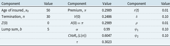All the relevant parameters defining the numerical example are reported in Table 2.

Table 2. Components in numerical example

In this example, the liabilities in state 1, $\hat{V}^1(t)$ , and in state 2, $\hat{V}^2(t)$ , are equal to zero, since the only payment is upon a transition between state 0 and 1, and therefore, there are no future payments on the contract if the policyholder is disabled or dead. Hence, the sum-at-risk, $\hat{R}^{12}(t)$ , (see Equation (4)) is equal to zero for all $t$ . The unfunded liabilities depend on $\mu _{12}(t)$ through the rate $l_{12}(t)$ , which is equal to zero since $\hat{R}^{12}(t)$ is equal to zero (see Equation (5)). Therefore, the expected unfunded liabilities do not depend on the transition intensity $\mu _{12}(t)$ , and it is only necessary to define the valuation basis by the two transition intensities $\hat{\mu }_{01}(t)$ and $\hat{\mu }_{02}(t)$ . We assume that $\hat{\mu }_{01}(t) = 0.95 \cdot \mathbb{E} \big [ \mu _{01}(t) \big ]$ and $\hat{\mu }_{02}(t) = 1.05 \cdot \mathbb{E} \big [ \mu _{02}(t) \big ]$ . Under these assumptions, the single premium, $\pi$ , is equal to 0.2989, while the initial reserve in the active state, $V(0)$ , is equal to 0.2486. We choose the target level for the conditional value-at-risk as $\tau = 0.5 \cdot CVaR_\alpha (L(n))$ .

We calculate the expected total costs, $\mathbb{E} \big [ TC \big ]$ , the expected total unfunded liabilities, $\mathbb{E}\big [ L^D(n) \big ]$ , and the conditional value-at-risk of the unfunded liabilities, $CVaR_\alpha (L(n))$ , with and without de-risking based on 5000 simulations of $\mu _{01}(t)$ and $\mu _{02}(t)$ . We study the de-risking option with and without the sum-at-risk and the de-risking swap with and without the sum-at-risk. The solution to the optimization problem is the pair $(h_{01}, h_{02})$ that minimizes the expected total costs.

Without de-risking, the expected total costs of the insurance company is 0.0279. The objective of the insurance company is to lower the expected total costs by investing in de-risking securities. The assets at initialization of the insurance contract are 0.2989 and the liabilities equal 0.2486, hence, the insurance company has $w_0 = 0.0503$ to buy de-risking at time 0. We plot the sums-at-risk for the transitions from Active to Disabled and from Active to Dead, respectively, in Fig. 2.

Figure 2. Sums-at-risk.

5.2.1 The de-risking option

The sum-at-risk from state 0 (Active) to state 1 (Disabled) is positive. Therefore, we consider the de-risking option with the European call option structure (Equation (7) with the sum-at-risk and Equation (9) without the sum-at-risk) for this transition. On the contrary, the sum-at-risk from state 0 (Active) to state 2 (Dead) is negative. Therefore, we consider the de-risking option with a European put option structure for this transition (Equation (8) with the sum-at-risk and Equation (10) without the sum-at-risk). In Fig. 3, we illustrate the expected total costs and the constraints from the optimization problem as functions of $h_{01}$ for a fixed value of $h_{02}$ . The expected total cost, the expected unfunded liabilities, and the conditional value-at-risk decrease in $h_{01}$ , while the hedging price increases in $h_{01}$ . The values of $h_{01}$ that meet the constraints in the optimization problem are the values where the conditional value-at-risk is lower than $\tau$ and where the hedging price is lower than $a_0$ . Since the expected total cost has a decreasing trend, the optimal solution for $h_{01}$ (given $h_{02}$ ) is given by the larger value of $h_{01}$ within the feasible region. This means that, given the longevity/mortality de-risking strategy, the insurance company should maximize the coverage from disability risk. We can see in Fig. 3 that the optimal values for $h_{01}$ are 0.47 and 2.27, respectively with and without sum-at-risk.

The optimal values of $h_{01}$ and $h_{02}$ for the de-risking options, when both are variable, are reported in Table 3. The expected total costs are negative in both cases. It can be concluded from Equation (13) that, thanks to the de-risking strategy, the weight of capital outflows (negative) is greater than the sum of the weights of capital inflows (positive) and the cost of the hedging strategy. We can also observe that the expected total cost is slightly lower for the de-risking option with the sum-at-risk than without the sum-at-risk. This indicates that the better hedge for the insurance company is to buy the de-risking option with the sum-at-risk than without, even if the difference is little. For both de-risk strategies, it is evident that the insurer must purchase higher amounts of disability options ( $h_{01}$ ) than longevity/mortality options ( $h_{02})$ . The resulting operational indication is that the insurer should give preeminence to reducing the disability risk over the longevity/mortality risk.

Table 3. Optimal amounts for the de-risking option

Figure 3. Illustration of the optimization problem for the de-risking option with and without the sum-at-risk. The colored dashed lines indicate the boundaries in the optimization problem, the black dashed lines indicate the feasible $h_{01}$ ’s, and the solid black line indicates the optimal $h_{01}$ .

5.2.3 De-risking in one scenario

The objective, when the insurance company chooses to buy de-risking securities, is to lower the total costs. It affects the total costs when the insurance company amortizes the unfunded liabilities with the $k(t)$ rate. Now, we consider one scenario and illustrate how the de-risking option decreases the rate $k(t)$ . The simulated path of $\mu _{01}(t)$ and $\mu _{02}(t)$ and the valuation basis $\hat{\mu }_{01}(t)$ and $\hat{\mu }_{02}(t)$ are illustrated in Fig. 5.

Table 4. Optimal amounts for the de-risking swap

Figure 4. Illustration of the optimization problem for the de-risking swap with and without the sum-at-risk. The colored dashed lines indicate the boundaries in the optimization problem, the black dashed lines indicate the feasible $h_{01}$ ’s, and the solid black line indicates the optimal $h_{01}$ .

Figure 5. Simulation of $\mu _{01}(t)$ and $\mu _{02}(t)$ (solid lines) and $\hat{\mu }_{01}(t)$ and $\hat{\mu }_{02}(t)$ (dashed lines).

In this scenario, the disability intensity $\mu _{01}(t)$ exceeds the valuation basis $\hat{\mu }_{01}(t)$ for $t \in [2, 8]$ and for $t \in [11, 17]$ , and since the sum-at-risk upon disability is positive, the insurance company faces a loss for these values of $t$ if it does not invest in de-risking securities. The mortality intensity $\mu _{02}(t)$ is lower than the valuation basis $\hat{\mu }_{02}(t)$ for all $t \lt 27$ , and since the sum-at-risk upon death is negative the insurance company faces a loss. We illustrate the rate $k(t)$ in Fig. 6 for the de-risking option and the de-risking swap with and without the sum-at-risk.

Figure 6. The rate $k(t)$ without de-risking and for the de-risking option and the de-risking swap with and without the sum-at-risk.

Fig. 6 illustrates that the de-risking option lowers the rate $k(t)$ such that, including de-risking, the insurance company faces a lower loss than without de-risking. For the de-risking option, the solid red line and the dashed red line in Fig. 6 are almost identical indicating that the optimal de-risking option with and without the sum-at-risk, respectively, results in an almost identical de-risking cash flow. We can see from Fig. 6 that the de-risking strategy based on options reduces the capital inflows ( $k\gt 0$ ) and leaves the capital outflows unchanged ( $k\lt 0$ ). The de-risking swap, results in a more stable rate $k(t)$ compared to the de-risking option and affects both the capital inflows and the capital outflows.