1. Introduction
Over the past decade, legged robotics has seen a dramatic growth in popularity largely due to showcases of impressive acrobatic stunts brought by many research groups as well as an ever-growing number of companies. However, beyond feats of agility, one major aspect that sparks the interest in legged robots is their capability to traverse natural (e.g., dirt, sand, snow, and gravel) or man-made landscapes (e.g., rubble and stairs) with great ease. Mastering locomotion would allow these robots to be effectively used in critical applications which currently still pose great danger to human lives, such as search and rescue operations in disaster areas, inspection of hazardous areas, and even space exploration. Legged locomotion is achieved by not only having well-built legs and body but also control systems that take locomotion principles into account. Effective control design inherently requires some knowledge of the expected system behavior to achieve a desired effect. This aspect is especially relevant for model-based control, where a model of the system dynamics is used to generate the control signals.
The model of the system dynamics can be obtained by applying first principles (e.g., Newton-Euler and Euler-Lagrange), using derived algorithms (e.g., Articulated Body Algorithm [Reference Featherstone1]), or by performing system identification. In any case, the chosen method should reflect the project requirements, which must take into account aspects such as system complexity and controller restrictions.
In recent years, Model Predictive Control (MPC) has become a popular scheme for legged locomotion planning and control, being extensively used by well-known research groups in the field [Reference Bledt, Powell, Katz, Di Carlo, Wensing and Kim2–Reference Rathod, Bratta, Focchi, Zanon, Villarreal, Semini and Bemporad9]. With MPC, dynamic model complexity plays a critical role in run-time performance. Neunert et al. [Reference Neunert, Stauble, Giftthaler, Bellicoso, Carius, Gehring, Hutter and Buchli8] employ a whole-body nonlinear MPC with an explicit soft contact model implemented by the Control Toolbox [Reference Giftthaler, Neunert, Stäuble and Buchli10] and full robot dynamics obtained from the RobCoGen [Reference Frigerio, Buchli and Caldwell11, Reference Giftthaler, Neunert, Stäuble, Frigerio, Semini and Buchli12] code generation framework. Hardware experiments done with two robots, HyQ [Reference Semini, Tsagarakis, Guglielmino, Focchi, Cannella and Caldwell13] and ANYmal [Reference Hutter, Gehring, Jud, Lauber, Bellicoso, Tsounis, Hwangbo, Bodie, Fankhauser, Bloesch, Diethelm, Bachmann, Melzer and Hoepflinger14], showed that despite the use of full robot dynamics, software design optimization and simplified contact dynamics allowed the proposed method to run at update rates over an order of magnitude higher than existing methods. As an alternative to full robot dynamics, approximations such as the centroidal [Reference Bledt, Powell, Katz, Di Carlo, Wensing and Kim2], single rigid body [Reference Di Carlo, Wensing, Katz, Bledt and Kim3–Reference Kim, Carlo, Katz, Bledt and Kim5, Reference Minniti, Grandia, Farshidian and Hutter7, Reference Rathod, Bratta, Focchi, Zanon, Villarreal, Semini and Bemporad9], and template-based dynamics (e.g., spring-loaded inverted pendulum and cart-table with flywheel [Reference Mastalli, Havoutis, Focchi, Caldwell and Semini6]) have been used to reduce complexity at the cost of accuracy. Rathod et al. [Reference Rathod, Bratta, Focchi, Zanon, Villarreal, Semini and Bemporad9] employ nonlinear MPC with an implicit hard contact model and single rigid body dynamics for locomotion planning. The use of a simplified model was key to decrease computational cost and allow for faster online re-planning that is required to deal with dynamic environments. Di Carlo et al. [Reference Di Carlo, Wensing, Katz, Bledt and Kim3] go a step further into simplifying the model, using MPC with linearized single rigid body dynamics. This choice allowed the controller to be formulated as a single convex optimization problem, which greatly improved solution speed and reliability as demonstrated in hardware experiments done with the MIT Cheetah 3 robot [Reference Bledt, Powell, Katz, Di Carlo, Wensing and Kim2]. One way to mitigate the reduced accuracy originated from using simplified models while not exactly fulfilling the simplifying assertions (e.g., massless legs) is by improving robustness. Grandia et al. [Reference Grandia, Farshidian, Ranftl and Hutter4] and Minniti et al. [Reference Minniti, Grandia, Farshidian and Hutter7] incorporate robustness mechanisms into MPC while using a kinodynamic model. Even though this model considers only the floating-base dynamics (single rigid body) along with the kinematics of each leg, the added robustness was able to compensate for modeling mismatches and external disturbances.
Contrasting with MPC, Whole Body Control (WBC), a powerful legged locomotion control scheme, strives for high model accuracy to generate consistent output signals, typically requiring the use of complete robot dynamics. Fahmi et al. [Reference Fahmi, Mastalli, Focchi and Semini15] use WBC to directly compute the actuation torques based on user velocity input and planned contact sequence while considering the full robot dynamics and an implicit hard contact model. Compared to their previous work using a simplified model (centroidal dynamics), hardware experiments showed enhanced locomotive capability, with the robot successfully traversing a wide range of challenging terrain. On the other hand, Kim et al. [Reference Kim, Carlo, Katz, Bledt and Kim5] employ WBC to compute the actuation torques based on the planned reaction force profile instead of body trajectories. This choice accommodates locomotion patterns with significant aerial phases, an important characteristic for high-speed running as demonstrated by experiments using the MIT Mini Cheetah [Reference Katz, Carlo and Kim16].
Few of the recent works from well-known research groups in the field utilize a dynamic model provided by readily available external libraries (e.g., RBDL [Reference Felis17]) or simulation software (e.g., MuJoCo [Reference Todorov, Erez and Tassa18], Raisim [Reference Hwangbo, Lee and Hutter19]), with most relying on custom in-house solutions. “Poor” computational performance with respect to specific practical requirements and inflexible model complexity of existing solutions are among the reasons which may justify this dependence. However, employing ready-to-use software still holds the potential benefit of abstraction, which can overcome the need to worry about implementation details, saving time, and effort. Abstraction works in our favor if it can be asserted that the software will function as intended, a condition that can be fulfilled by offering enough clarity with regard to its inner workings, such as providing comprehensive and well-founded documentation, practical working examples, and referring to comparative analyses with well-established methods.
In this paper, we characterize the quadruped robot and contact dynamics that will compose our in-house simulator to be used for prototyping locomotion control schemes applied to quadruped robots. The proposed simulator computes the robot dynamics using the Recursive Newton-Euler Algorithm (RNEA) along with the Composite-Rigid-Body Algorithm (CRBA), similar to their definition in ref. [Reference Featherstone1] but with a few modifications to make certain aspects relevant for contact detection and control more easily accessible. With respect to the contact dynamics, it uses a compliant (nonlinear spring-damper) contact force model alongside stick-slip friction. Evaluation of the proposed simulator was done by implementing a simple PD-independent joint controller to track a desired leg trajectory, synthesized by a foot trajectory generator we proposed in our previous work [Reference De Paula, Godoy and Becerra-Vargas20], and comparing characteristic locomotion signals such as the trunk pose and the contact forces, with the same robot and controller implemented using the MuJoCo simulation software. Results showed very similar behavior for both simulators, especially with regard to the contact detection, despite the significantly different contact models.
1.1. Main contributions
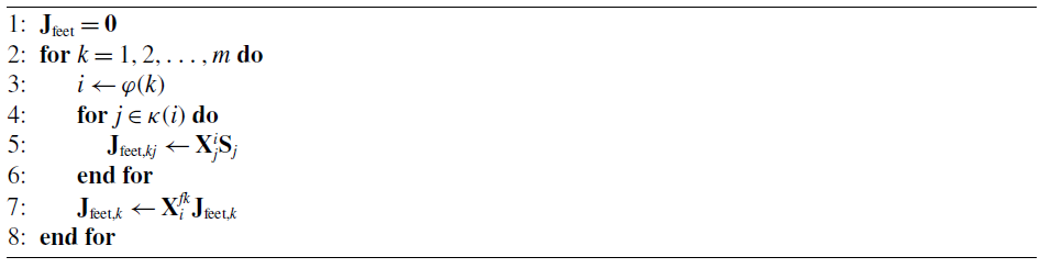
Since our objective is to develop a ready-to-use software that embraces the benefits of abstraction while asserting that it will function as intended, our work’s main contribution can be stated as defining a transparent and well-founded simulator that is capable of being used for prototyping locomotion control schemes applied to legged robots. Additionally, with a focus on easing the development of model-based control schemes, we consider two minor contributions: (1) the definition of algorithms derived from the RNEA that separately compute the quadratic velocity and gravity terms, making them easily accessible for use in specialized control schemes (e.g., gravity compensation); and (2) definition of an algorithm to compute the (geometric) Jacobian matrix of the feet, typically required when a task space specification (e.g., desired cartesian coordinates of the feet) must be converted into a joint torque command, by means of a recursive formulation that relies on traversing the support path of each leg of the robot.
2. Definitions and notation
In this work, scalar quantities are depicted with medium italic lowercase Latin or Greek letters (e.g., gravitational acceleration
 $g$
and friction coefficient
$g$
and friction coefficient
 $\mu$
), vectors are depicted with bold-face upright (or italic for three-dimensional vectors) lowercase Latin or Greek letters (e.g., spatial velocity
$\mu$
), vectors are depicted with bold-face upright (or italic for three-dimensional vectors) lowercase Latin or Greek letters (e.g., spatial velocity
 $\mathbf{v}$
, position
$\mathbf{v}$
, position
 $\boldsymbol{p}$
, and angular velocity
$\boldsymbol{p}$
, and angular velocity
 $\boldsymbol{\omega }$
), and matrices are depicted with bold-face upright uppercase Latin letters (e.g., rotation matrix
$\boldsymbol{\omega }$
), and matrices are depicted with bold-face upright uppercase Latin letters (e.g., rotation matrix
 $\mathbf{R}$
). As an exception, bold-face lowercase Latin or Greek letters with a tilde represent the skew-symmetric matrix (as defined in Appendix A) correspondent to that vector (e.g.,
$\mathbf{R}$
). As an exception, bold-face lowercase Latin or Greek letters with a tilde represent the skew-symmetric matrix (as defined in Appendix A) correspondent to that vector (e.g.,
 $\tilde{\boldsymbol{\omega }}$
is the skew-symmetric matrix of vector
$\tilde{\boldsymbol{\omega }}$
is the skew-symmetric matrix of vector
 $\boldsymbol{\omega }$
). In the absence of the right superscript, which denotes the frame of reference, consider the variable expressed in its respective body frame. Additionally,
$\boldsymbol{\omega }$
). In the absence of the right superscript, which denotes the frame of reference, consider the variable expressed in its respective body frame. Additionally,
 $\mathbf{0}$
represents either a zero vector or zero-filled matrix (depending on the context), while
$\mathbf{0}$
represents either a zero vector or zero-filled matrix (depending on the context), while
 $\mathbf{1}$
represents the identity matrix.
$\mathbf{1}$
represents the identity matrix.
2.1. Quadruped robot
The quadruped robot model described in this section is based on the 18 degrees-of-freedom (DOF) torque-controlled MIT Mini Cheetah [Reference Katz, Carlo and Kim16], a small and low-cost robot designed and built for dynamic locomotion with readily available geometrical and inertial data through the MIT Biomimetic Robotics Lab GitHub repository [21]. Figure 1 presents a three-dimensional rendering of the quadruped robot showing its geometrical structure, two of its frames of reference (the trunk frame and the world frame), and the characteristic DOF of the leg. The trunk frame
 $\{0\}$
represents a frame of reference attached to the robot’s trunk, while the world frame
$\{0\}$
represents a frame of reference attached to the robot’s trunk, while the world frame
 $\{W\}$
is an inertial frame of reference attached to the ground. The four legs are identical, each having a 3-DOF open kinematic chain topology with the base attached to the robot’s trunk.
$\{W\}$
is an inertial frame of reference attached to the ground. The four legs are identical, each having a 3-DOF open kinematic chain topology with the base attached to the robot’s trunk.
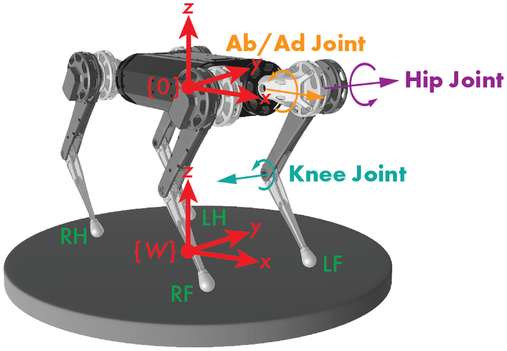
Figure 1. Three-dimensional rendering of the quadruped robot model with two of its frames of reference and the characteristic degrees-of-freedom of the leg.
As illustrated in Fig. 1, from the base to the feet of a single leg, we have the abduction/adduction joint, the hip joint, and the knee joint. In this work, each leg is identified by a unique two-letter acronym based on the relative position of its base frame with respect to the trunk frame; that is, LF, RF, LH, and RH, referring to the left foreleg, to the right foreleg, to the left hindleg, and to the right hindleg, respectively.
2.2. Rigid bodies and connectivity
Figure 2a presents a simplified diagram with the corresponding numbers used to represent the 13 rigid bodies (
 $n_b = 13$
) that compose the quadruped robot. The system topology can be expressed as a connectivity graph, an undirected and connected graph where the nodes represent bodies and line segments represent the joints. The floating-base connectivity graph respective to the quadruped robot is presented in Fig. 2b. Note that the robot has 13 joints numbered from 0 to 12, where joint 0 (not shown in the graph) is a spatial 6-DOF joint while the remaining are all revolute joints.
$n_b = 13$
) that compose the quadruped robot. The system topology can be expressed as a connectivity graph, an undirected and connected graph where the nodes represent bodies and line segments represent the joints. The floating-base connectivity graph respective to the quadruped robot is presented in Fig. 2b. Note that the robot has 13 joints numbered from 0 to 12, where joint 0 (not shown in the graph) is a spatial 6-DOF joint while the remaining are all revolute joints.
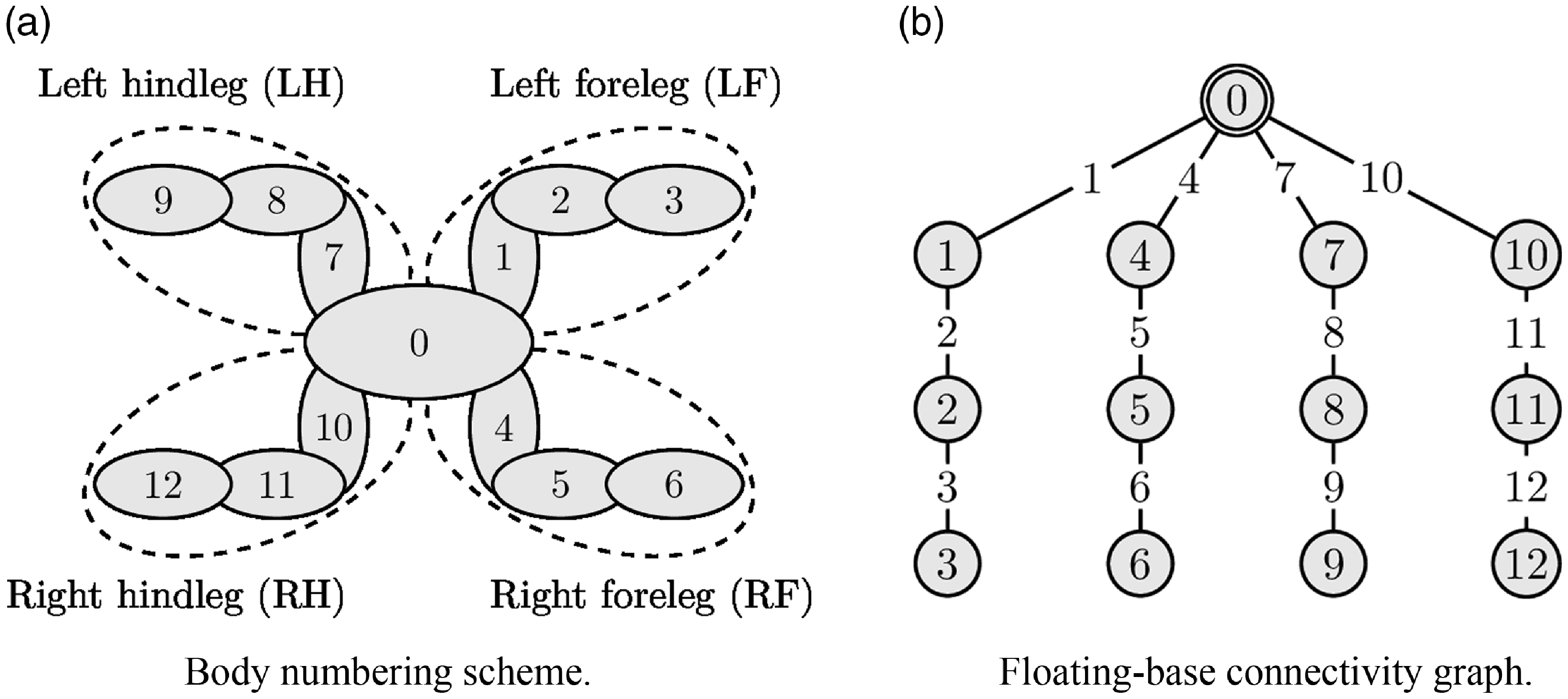
Figure 2. Simplified diagrams showing the body numbering scheme and the connectivity graph respective to the quadruped robot model.
The floating-base system with open-chain limbs that composes the quadruped robot has a tree-structured kinematic chain where each branch of the tree can be intuitively traversed using recursion. A systematic method to index the bodies in the rigid-body system must be established to convert this recursion into an iterative process, which is more computationally efficient. Based on the connectivity graph, the predecessor array pred and successor array succ can be defined. Starting from joint 1, each element of the predecessor array pred
 $(i)$
represents the body preceding joint
$(i)$
represents the body preceding joint
 $i$
, while for the successor array each element succ
$i$
, while for the successor array each element succ
 $(i)$
represents the body succeeding joint
$(i)$
represents the body succeeding joint
 $i$
. From the connectivity graph (Fig. 2b), the predecessor and successor arrays can be defined as:
$i$
. From the connectivity graph (Fig. 2b), the predecessor and successor arrays can be defined as:
When combined, the predecessor and successor arrays describe all the connected pairs of rigid bodies in the tree-structured kinematic chain. One such combination yields the parent array
 $\lambda$
. Each element
$\lambda$
. Each element
 $\lambda (i)$
represents the parent of body
$\lambda (i)$
represents the parent of body
 $i$
, being calculated as [Reference Featherstone1]:
$i$
, being calculated as [Reference Featherstone1]:
Applying relation (2) to predecessor and successor arrays defined in (1) results in the parent array:
 \begin{equation} \lambda = \lbrace 0, 1, 2, 0, 4, 5, 0, 7, 8, 0, 10, 11 \rbrace . \end{equation}
Three other useful parameters which can be defined are the support set
 $\kappa (i)$
, the set of all joints in between body
$\kappa (i)$
, the set of all joints in between body
 $i$
and the root, the child set
$i$
and the root, the child set
 $\mu (i)$
, the set of children of body
$\mu (i)$
, the set of children of body
 $i$
, and the subtree set
$i$
, and the subtree set
 $\nu (i)$
, the set of bodies in the subtree rooted at body
$\nu (i)$
, the set of bodies in the subtree rooted at body
 $i$
.
$i$
.
2.3. Traversing the kinematic chain
Given the robot’s tree-structured kinematic chain, traversal is done using either an outward or an inward pass. In an outward pass, we start at the root, going from parent body
 $\lambda (i)$
to child body
$\lambda (i)$
to child body
 $i$
until all the leaf nodes have been reached. For an inward pass, we begin at the leaf nodes and follow the opposite path, going from child body
$i$
until all the leaf nodes have been reached. For an inward pass, we begin at the leaf nodes and follow the opposite path, going from child body
 $i$
to its parent body
$i$
to its parent body
 $\lambda (i)$
until all paths have arrived at the root. Only a single outward pass is used for the kinematics, while both an inward and outward pass are required for the dynamics.
$\lambda (i)$
until all paths have arrived at the root. Only a single outward pass is used for the kinematics, while both an inward and outward pass are required for the dynamics.
2.4. Motion and force transforms
Let
 $\{A\}$
and
$\{A\}$
and
 $\{B\}$
be coordinate frames fixed to a single rigid body and let
$\{B\}$
be coordinate frames fixed to a single rigid body and let
 $\mathbf{v}_A = (\boldsymbol{\omega }_A, \boldsymbol{v}_A)$
and
$\mathbf{v}_A = (\boldsymbol{\omega }_A, \boldsymbol{v}_A)$
and
 $\mathbf{v}_B = (\boldsymbol{\omega }_B, \boldsymbol{v}_B)$
be their respective spatial velocity vectors, where
$\mathbf{v}_B = (\boldsymbol{\omega }_B, \boldsymbol{v}_B)$
be their respective spatial velocity vectors, where
 $\boldsymbol{v}$
is the linear velocity and
$\boldsymbol{v}$
is the linear velocity and
 $\boldsymbol{\omega }$
is the angular velocity. The spatial velocity
$\boldsymbol{\omega }$
is the angular velocity. The spatial velocity
 $\mathbf{v}_B$
can be computed from
$\mathbf{v}_B$
can be computed from
 $\mathbf{v}_A$
by means of the motion transformation matrix
$\mathbf{v}_A$
by means of the motion transformation matrix
 $\mathbf{X}_A^B$
, which applies the required translation and rotation procedures to transform the spatial velocity vector from
$\mathbf{X}_A^B$
, which applies the required translation and rotation procedures to transform the spatial velocity vector from
 $\{A\}$
to
$\{A\}$
to
 $\{B\}$
; that is,
$\{B\}$
; that is,
 \begin{equation} \mathbf{v}_B = \mathbf{X}_A^B \mathbf{v}_A. \end{equation}
Given the rotation matrix
 $\mathbf{R}_A^B$
and the absolute position vectors of the origins of each frame
$\mathbf{R}_A^B$
and the absolute position vectors of the origins of each frame
 $\boldsymbol{p}_{O_{A}}^A$
and
$\boldsymbol{p}_{O_{A}}^A$
and
 $\boldsymbol{p}_{O_{B}}^A$
expressed in
$\boldsymbol{p}_{O_{B}}^A$
expressed in
 $\{A\}$
, the motion transformation matrix
$\{A\}$
, the motion transformation matrix
 $\mathbf{X}_A^B$
can be expressed as:
$\mathbf{X}_A^B$
can be expressed as:
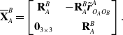
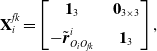
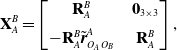 \begin{equation} \mathbf{X}_A^B = \begin{bmatrix} \mathbf{R}_A^B\;\;\;\; & \mathbf{0}_{3 \times 3}\\[5pt] -\mathbf{R}_A^B\tilde{\boldsymbol{r}}_{O_{A}O_{B}}^A\;\;\;\; & \mathbf{R}_A^B \end{bmatrix}, \end{equation}
where
 $\mathbf{0}_{3 \times 3}$
is a zero-filled 3-by-3 matrix and
$\mathbf{0}_{3 \times 3}$
is a zero-filled 3-by-3 matrix and
 $\tilde{\boldsymbol{r}}_{O_{A}O_{B}}^A$
is the skew-symmetric matrix (Appendix A) associated with the displacement vector
$\tilde{\boldsymbol{r}}_{O_{A}O_{B}}^A$
is the skew-symmetric matrix (Appendix A) associated with the displacement vector
 $\boldsymbol{r}_{O_{A}O_{B}}^A = \boldsymbol{p}_{O_{B}}^A-\boldsymbol{p}_{O_{A}}^A$
.
$\boldsymbol{r}_{O_{A}O_{B}}^A = \boldsymbol{p}_{O_{B}}^A-\boldsymbol{p}_{O_{A}}^A$
.
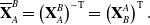
With respect to spatial forces, a similar relation can be established. The force transformation matrix
 $\mathbf{\overline{X}}_A^B$
correlates spatial force vector
$\mathbf{\overline{X}}_A^B$
correlates spatial force vector
 $\mathbf{f}_B = (\boldsymbol{n}_B, \boldsymbol{f}_B)$
to
$\mathbf{f}_B = (\boldsymbol{n}_B, \boldsymbol{f}_B)$
to
 $\mathbf{f}_A = (\boldsymbol{n}_A, \boldsymbol{f}_A)$
, where
$\mathbf{f}_A = (\boldsymbol{n}_A, \boldsymbol{f}_A)$
, where
 $\boldsymbol{n}$
is the moment and
$\boldsymbol{n}$
is the moment and
 $\boldsymbol{f}$
is the force acting at origin of their respective frame of reference, such that
$\boldsymbol{f}$
is the force acting at origin of their respective frame of reference, such that
 \begin{equation} \mathbf{f}_B = \mathbf{\overline{X}}_A^B \mathbf{f}_A. \end{equation}
Following the same assumptions used to compute the motion transformation matrix (5), the force transformation matrix
 $\mathbf{\overline{X}}_A^B$
can be expressed as:
$\mathbf{\overline{X}}_A^B$
can be expressed as:
 \begin{equation} \mathbf{\overline{X}}_A^B = \begin{bmatrix} \mathbf{R}_A^B\;\;\;\; & -\mathbf{R}_A^B\tilde{\boldsymbol{r}}_{O_{A}O_{B}}^A\\[5pt] \mathbf{0}_{3 \times 3}\;\;\;\; & \mathbf{R}_A^B \end{bmatrix}. \end{equation}
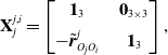
Note that the force transformation matrix can be computed from the motion transformation matrix and vice versa, that is,
 \begin{equation} \mathbf{\overline{X}}_A^B = \left (\mathbf{X}_A^B\right )^{-\text{T}} = \left (\mathbf{X}_B^A\right )^{\text{T}}. \end{equation}
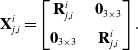
3. Tree-structured kinematics
The kinematics requires an outward pass to traverse the kinematic chain and calculate the spatial velocity of each body in the system with respect to the root node. Computing the motion transformation matrix (5) can be done in two consecutive stages: (i) a translation to the location of the next active joint, here represented by the fictitious joint frame
 $\{\lambda (i),i\}$
which represents joint
$\{\lambda (i),i\}$
which represents joint
 $i$
fixed to body
$i$
fixed to body
 $\lambda (i)$
, followed by (ii) a rotation to account for the joint motion (and possible offset). Letting
$\lambda (i)$
, followed by (ii) a rotation to account for the joint motion (and possible offset). Letting
 $j = \lambda (i)$
represent the parent body, the first stage transform
$j = \lambda (i)$
represent the parent body, the first stage transform
 $\mathbf{X}_{j}^{j,i}$
can be defined as:
$\mathbf{X}_{j}^{j,i}$
can be defined as:
 \begin{equation} \mathbf{X}_{j}^{j,i} = \begin{bmatrix} \mathbf{1}_3\;\;\;\; & \mathbf{0}_{3 \times 3} \\[5pt] -\tilde{\boldsymbol{r}}_{O_jO_i}^j\;\;\;\; & \mathbf{1}_3 \end{bmatrix}, \end{equation}
where
 $\mathbf{1}_3$
is a
$\mathbf{1}_3$
is a
 $3 \times 3$
identity matrix. The following second stage transform
$3 \times 3$
identity matrix. The following second stage transform
 $\mathbf{X}_{j,i}^{i}$
can be expressed as:
$\mathbf{X}_{j,i}^{i}$
can be expressed as:
 \begin{equation} \mathbf{X}_{j,i}^{i} = \begin{bmatrix} \mathbf{R}_{j,i}^{i}\;\;\;\; & \mathbf{0}_{3 \times 3} \\[5pt] \mathbf{0}_{3 \times 3}\;\;\;\; & \mathbf{R}_{j,i}^{i} \end{bmatrix}. \end{equation}
Note that the first stage yields a constant matrix that depends only on the system’s geometry, while the second stage is a function of the corresponding joint variable (e.g., the joint angle for revolute joints). The resulting motion transformation
 $\mathbf{X}_{j}^{i}$
from the parent body frame
$\mathbf{X}_{j}^{i}$
from the parent body frame
 $\{j\}$
to the current body frame
$\{j\}$
to the current body frame
 $\{i\}$
is given by:
$\{i\}$
is given by:
 \begin{equation} \mathbf{X}_{j}^{i} = \mathbf{X}_{j,i}^{i} \mathbf{X}_{j}^{j,i}. \end{equation}
With this transform, the motion transformation matrix
 $\mathbf{X}_{0}^{i}$
from body
$\mathbf{X}_{0}^{i}$
from body
 $0$
(in this case the root node) to each body
$0$
(in this case the root node) to each body
 $i$
can be computed as:
$i$
can be computed as:
 \begin{equation} \mathbf{X}_{0}^{i} = \mathbf{X}_{j}^{i}\mathbf{X}_{0}^{j}. \end{equation}
Given the joint motion subspace matrix
 $\mathbf{S}_i$
, which confines the spatial joint velocity
$\mathbf{S}_i$
, which confines the spatial joint velocity
 $i$
to the motion subspace defined by the joint DOF, the spatial velocity
$i$
to the motion subspace defined by the joint DOF, the spatial velocity
 $\mathbf{v}_i$
of body
$\mathbf{v}_i$
of body
 $i$
can be formulated as:
$i$
can be formulated as:
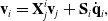 \begin{equation} \mathbf{v}_i = \mathbf{X}^i_j \mathbf{v}_j + \mathbf{S}_i \dot{\mathbf{q}}_i, \end{equation}
where
 $\dot{\mathbf{q}}_i$
is the joint velocity vector. In the case of a spatial 6-DOF joint,
$\dot{\mathbf{q}}_i$
is the joint velocity vector. In the case of a spatial 6-DOF joint,
 $\mathbf{S}_i = \mathbf{1}_6$
and the joint velocity is a six-dimensional vector (angular and linear velocity), while for a revolute joint, the joint velocity is a scalar (equivalent to the joint angle derivative) and
$\mathbf{S}_i = \mathbf{1}_6$
and the joint velocity is a six-dimensional vector (angular and linear velocity), while for a revolute joint, the joint velocity is a scalar (equivalent to the joint angle derivative) and
 $\mathbf{S}_i = [\begin{smallmatrix}0 & 0 & 1 & 0 & 0 & 0\end{smallmatrix}]^{\mathrm{T}}$
assuming the axis of rotation and its sense matches the z-axis of the body coordinate system.
$\mathbf{S}_i = [\begin{smallmatrix}0 & 0 & 1 & 0 & 0 & 0\end{smallmatrix}]^{\mathrm{T}}$
assuming the axis of rotation and its sense matches the z-axis of the body coordinate system.
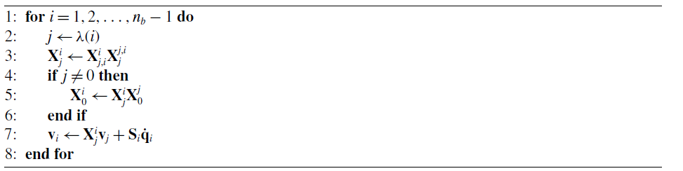
Algorithm 1 presents the outward pass traversal used to compute each motion transformation matrix
 $\mathbf{X}_{j}^{i}$
and
$\mathbf{X}_{j}^{i}$
and
 $\mathbf{X}_{0}^{i}$
as well as the spatial velocity
$\mathbf{X}_{0}^{i}$
as well as the spatial velocity
 $\mathbf{v}_i$
. Note that the conditional statement in line 4 is required only because the expression in line 3 already handles the transforms relative to the bodies directly connected to the body 0.
$\mathbf{v}_i$
. Note that the conditional statement in line 4 is required only because the expression in line 3 already handles the transforms relative to the bodies directly connected to the body 0.
Algorithm 1. Kinematics computation
3.1. Transform to the world frame
To correlate the motion transformation matrices to the inertial world frame, we define the motion transformation matrix
 $\mathbf{X}_W^0$
from the world frame
$\mathbf{X}_W^0$
from the world frame
 $\{W\}$
to the trunk frame
$\{W\}$
to the trunk frame
 $\{0\}$
as:
$\{0\}$
as:
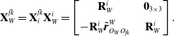
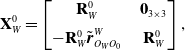 \begin{equation} \mathbf{X}_W^0 = \begin{bmatrix} \mathbf{R}_W^0\;\;\;\; & \mathbf{0}_{3 \times 3} \\[5pt] -\mathbf{R}_W^0 \tilde{\boldsymbol{r}}_{O_WO_0}^W \;\;\;\; & \mathbf{R}_W^0 \end{bmatrix}, \end{equation}
where
 $\boldsymbol{r}_{O_WO_0}^W$
represents the displacement vector from the world frame to the trunk frame (cartesian coordinates of the trunk frame origin expressed in the world frame) and
$\boldsymbol{r}_{O_WO_0}^W$
represents the displacement vector from the world frame to the trunk frame (cartesian coordinates of the trunk frame origin expressed in the world frame) and
 $\mathbf{R}_0^W ={\left ({\mathbf{R}_W^0}\right )}^{\mathrm{T}}$
represents the orientation of the trunk frame with respect to the world frame. With
$\mathbf{R}_0^W ={\left ({\mathbf{R}_W^0}\right )}^{\mathrm{T}}$
represents the orientation of the trunk frame with respect to the world frame. With
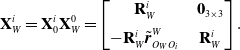
 $\mathbf{X}_W^0$
, the motion transformation matrix from the world frame
$\mathbf{X}_W^0$
, the motion transformation matrix from the world frame
 $\{W\}$
to each body
$\{W\}$
to each body
 $i$
can be computed by pre-multiplying
$i$
can be computed by pre-multiplying
 $\mathbf{X}_0^i$
, that is,
$\mathbf{X}_0^i$
, that is,
 \begin{equation} \mathbf{X}_W^i = \mathbf{X}_0^i \mathbf{X}_W^0 = \begin{bmatrix} \mathbf{R}_W^i \;\;\;\; & \mathbf{0}_{3 \times 3} \\[5pt] -\mathbf{R}_W^i \tilde{\boldsymbol{r}}_{O_WO_i}^W \;\;\;\; & \mathbf{R}_W^i \end{bmatrix}. \end{equation}
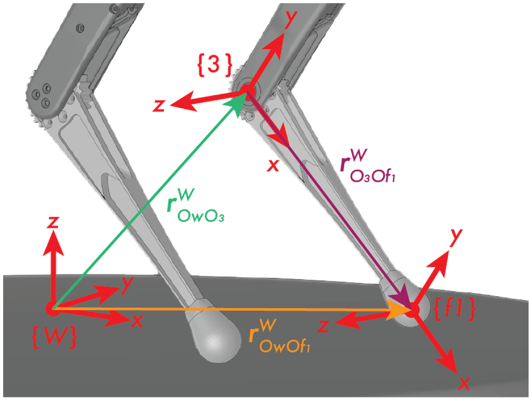
Figure 3. Foot frame pose components for the left foreleg in the quadruped robot.
3.2. Foot position
As the contact dynamics algorithm uses the foot position for contact detection and contact force generation, its relation to the joint variables must be established. Let the feet index array
 $\varphi$
represent the bodies rigidly attached to each foot frame, where
$\varphi$
represent the bodies rigidly attached to each foot frame, where
 $i=\varphi (k)$
is the body correspondent to foot
$i=\varphi (k)$
is the body correspondent to foot
 $k$
, and let the foot frame
$k$
, and let the foot frame
 $\{fk\}$
be located where the ground contact forces will act upon, with its orientation being the same as its respective body frame (as shown in Fig. 3 for the left foreleg). Then, the motion transformation matrix from the body frame
$\{fk\}$
be located where the ground contact forces will act upon, with its orientation being the same as its respective body frame (as shown in Fig. 3 for the left foreleg). Then, the motion transformation matrix from the body frame
 $\{i\}$
to the foot frame
$\{i\}$
to the foot frame
 $\{fk\}$
can be seen as a pure translation, that is,
$\{fk\}$
can be seen as a pure translation, that is,
 \begin{equation} \mathbf{X}_i^{fk} = \begin{bmatrix} \mathbf{1}_3 \;\;\;\; & \mathbf{0}_{3 \times 3} \\[5pt] - \tilde{\boldsymbol{r}}_{O_{i}O_{fk}}^i \;\;\;\; & \mathbf{1}_3 \end{bmatrix}, \end{equation}
where
 $|\boldsymbol{r}_{O_{i}O_{fk}}^i|$
is equivalent to the length of the last link of leg
$|\boldsymbol{r}_{O_{i}O_{fk}}^i|$
is equivalent to the length of the last link of leg
 $k$
. As a result, the motion transformation matrix from the world frame to the foot frame can be expressed as:
$k$
. As a result, the motion transformation matrix from the world frame to the foot frame can be expressed as:
 \begin{equation} \mathbf{X}_W^{fk} = \mathbf{X}_i^{fk} \mathbf{X}_W^{i} = \begin{bmatrix} \mathbf{R}_W^{i} \;\;\;\; & \mathbf{0}_{3 \times 3} \\[5pt] -\mathbf{R}_W^{i}\tilde{\boldsymbol{r}}_{O_{W}O_{fk}}^W \;\;\;\; & \mathbf{R}_W^{i} \end{bmatrix}. \end{equation}
Note that the foot displacement vector
 $\boldsymbol{r}_{O_{W}O_{fk}}^W$
can be extracted from the first block-column, second block-row term of (17) by deconstructing its skew-symmetric matrix which can be formulated as:
$\boldsymbol{r}_{O_{W}O_{fk}}^W$
can be extracted from the first block-column, second block-row term of (17) by deconstructing its skew-symmetric matrix which can be formulated as:
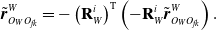 \begin{equation} \tilde{\boldsymbol{r}}_{O_{W}O_{fk}}^W = -\left (\mathbf{R}_W^{i}\right )^{\text{T}} \left (-\mathbf{R}_W^{i}\tilde{\boldsymbol{r}}_{O_{W}O_{fk}}^W\right ). \end{equation}
4. Tree-structured dynamics
The proposed simulator builds the quadruped robot’s equations of motion (EoM) using the RNEA to compute the bias force (i.e., quadratic velocity, gravitational, and external wrench terms) and the CRBA to compute the inertia matrix. Our approach is very similar to the inertia matrix method presented in ref. [Reference Featherstone1] applied to floating-base robots, with the exception that the RNEA was partitioned into separate modules to isolate the contribution of the quadratic velocity terms, gravitational terms, and external forces, making them more accessible for future control applications. Note that throughout this section, we consider that the velocity transformation matrices and spatial velocities of each body are readily available, being previously computed using Algorithm 1. In this section, unless explicitly stated otherwise, consider index
 $j$
as representing the parent body index, that is,
$j$
as representing the parent body index, that is,
 $j = \lambda (i)$
.
$j = \lambda (i)$
.
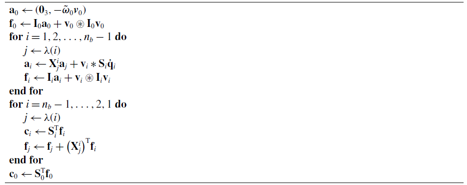
4.1. Quadratic velocity terms
As the name implies, the quadratic velocity terms are quadratic (nonlinear) functions of spatial velocity which comprise wrenches in the EoM. In our case, these terms originate only from inertial effects (i.e., centrifugal and Coriolis forces). For body
 $i$
with spatial velocity
$i$
with spatial velocity
 $\mathbf{v}_i$
, the spatial acceleration
$\mathbf{v}_i$
, the spatial acceleration
 $\mathbf{a}_i$
due to the quadratic velocity terms, assuming that the motion subspace matrix
$\mathbf{a}_i$
due to the quadratic velocity terms, assuming that the motion subspace matrix
 $\mathbf{S}_i$
is constant, can be computed as:
$\mathbf{S}_i$
is constant, can be computed as:
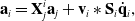 \begin{equation} \mathbf{a}_i = \mathbf{X}_{j}^i \mathbf{a}_{j} + \mathbf{v}_{i} \ast \mathbf{S}_i \dot{\mathbf{q}}_i, \end{equation}
where
 $\ast$
is the twist cross-product operator described in Appendix A. From the spatial velocity
$\ast$
is the twist cross-product operator described in Appendix A. From the spatial velocity
 $\mathbf{v}_i$
and the spatial acceleration
$\mathbf{v}_i$
and the spatial acceleration
 $\mathbf{a}_i$
, the wrench
$\mathbf{a}_i$
, the wrench
 $\mathbf{f}_i$
, which accounts for the contribution of body
$\mathbf{f}_i$
, which accounts for the contribution of body
 $i$
to the quadratic velocity terms, results from
$i$
to the quadratic velocity terms, results from
 \begin{equation} \mathbf{f}_i = \mathbf{I}_i\mathbf{a}_i + \mathbf{v}_i \circledast \mathbf{I}_i \mathbf{v}_i, \end{equation}
where
 $\circledast$
is the wrench cross-product operator described in Appendix A and
$\circledast$
is the wrench cross-product operator described in Appendix A and
 $\mathbf{I}_i$
is the spatial inertia tensor of body
$\mathbf{I}_i$
is the spatial inertia tensor of body
 $i$
referred to its respective body frame.Footnote
1
$i$
referred to its respective body frame.Footnote
1
The preceding computations can be done in the outward pass alongside the forward kinematics. To obtain the net force acting on each body due to quadratic velocity terms, an additional inward pass is required to propagate wrenches applied to each child body in the kinematic chain. This operation can be interpreted as an update to the quadratic velocity terms, being expressed as:
 \begin{equation} \mathbf{f}_{j} \gets \mathbf{f}_{j} +{\left (\mathbf{X}_{j}^i\right )}^{\mathrm{T}} \mathbf{f}_i. \end{equation}
With the help of the joint motion subspace matrix
 $\mathbf{S}_i$
, it is possible to convert the quadratic velocity terms into their joint-space counterpart
$\mathbf{S}_i$
, it is possible to convert the quadratic velocity terms into their joint-space counterpart
 $\mathbf{c}_i$
, such that
$\mathbf{c}_i$
, such that
 \begin{equation} \mathbf{c}_i = \mathbf{S}_i^{\text{T}}\mathbf{f}_{i}. \end{equation}
Algorithm 2 summarizes the joint-space quadratic velocity terms computation, defining the function used to compute the system joint-space quadratic velocity vector
 $\mathbf{c} = (\mathbf{c}_0, \mathbf{c}_1, \mathbf{c}_2, \ldots, \mathbf{c}_{12})$
. It is worth noting that at the start of the algorithm, we explicitly initialize the trunk spatial acceleration with only its the velocity-product term.
$\mathbf{c} = (\mathbf{c}_0, \mathbf{c}_1, \mathbf{c}_2, \ldots, \mathbf{c}_{12})$
. It is worth noting that at the start of the algorithm, we explicitly initialize the trunk spatial acceleration with only its the velocity-product term.
Algorithm 2. Quadratic velocity terms
4.2. Gravitational terms
The procedure required to compute the gravitational forces is very similar to the quadratic velocity terms computation, relying on an outward pass to account for the individual contribution of each body and an inward pass to propagate the succeeding wrenches and generate the joint-space terms. The outward pass involves computing the spatial acceleration
 $\mathbf{a}_i$
and the resulting wrench
$\mathbf{a}_i$
and the resulting wrench
 $\mathbf{f}_i$
such that
$\mathbf{f}_i$
such that
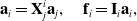 \begin{equation} \mathbf{a}_i = \mathbf{X}_j^i \mathbf{a}_j,\quad \mathbf{f}_i = \mathbf{I}_i \mathbf{a}_i, \end{equation}
while the inward pass updates each wrench exactly as (22), with the joint-space gravity terms being expressed as:
 \begin{equation} \mathbf{g}_{i} = \mathbf{S}_i^{\mathrm{T}} \mathbf{f}_i. \end{equation}
Algorithm 3 summarizes the joint-space gravity terms computation, defining the function used to compute the system joint-space gravitational forces vector
 $\mathbf{g} = (\mathbf{g}_0, \mathbf{g}_1, \mathbf{g}_2, \ldots, \mathbf{g}_{12})$
. Note that as in ref. [Reference Featherstone1], gravity is not added as an external force but instead is introduced through a fictitious upward acceleration applied to the trunk
$\mathbf{g} = (\mathbf{g}_0, \mathbf{g}_1, \mathbf{g}_2, \ldots, \mathbf{g}_{12})$
. Note that as in ref. [Reference Featherstone1], gravity is not added as an external force but instead is introduced through a fictitious upward acceleration applied to the trunk
 $\mathbf{a}_0 = -(\mathbf{0}_{3}, \mathbf{R}_W^0\boldsymbol{g}_0)$
, where
$\mathbf{a}_0 = -(\mathbf{0}_{3}, \mathbf{R}_W^0\boldsymbol{g}_0)$
, where
 $\boldsymbol{g}_0 = (0,0,-9.807) \mathrm{\ m/s^2}$
. Since the gravity acceleration vector
$\boldsymbol{g}_0 = (0,0,-9.807) \mathrm{\ m/s^2}$
. Since the gravity acceleration vector
 $\boldsymbol{g}_0$
is expressed in the world frame, it must first be transformed into the body frame to be included in the algorithm.
$\boldsymbol{g}_0$
is expressed in the world frame, it must first be transformed into the body frame to be included in the algorithm.
Algorithm 3. Gravitational terms
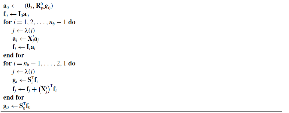
4.3. External wrenches
Computing the external wrenches (Algorithm 4) is even simpler than the gravitational terms. The outward pass computes the resulting external wrenches
 $\mathbf{f}_{i}$
applied to body
$\mathbf{f}_{i}$
applied to body
 $i$
at
$i$
at
 $O_i$
expressed in frame
$O_i$
expressed in frame
 $\{i\}$
from those applied at
$\{i\}$
from those applied at
 $O_{F_i}$
expressed in frame
$O_{F_i}$
expressed in frame
 $\{F_i\}$
, that is,
$\{F_i\}$
, that is,
 $\mathbf{f}_{\text{ext}i}^{F_i}$
. The inward pass performs the wrench propagation and generates the joint-space terms
$\mathbf{f}_{\text{ext}i}^{F_i}$
. The inward pass performs the wrench propagation and generates the joint-space terms
 $\boldsymbol{\tau }_{\text{e}i}$
. In this work, only the external forces originated from the contact dynamics and the active joint torques
$\boldsymbol{\tau }_{\text{e}i}$
. In this work, only the external forces originated from the contact dynamics and the active joint torques
 $\boldsymbol{\tau }$
are accounted for, with a detailed discussion regarding how to compute the former presented in Section 5. Note that the active joint torques
$\boldsymbol{\tau }$
are accounted for, with a detailed discussion regarding how to compute the former presented in Section 5. Note that the active joint torques
 $\boldsymbol{\tau }$
are directly added to the EoM using the selection matrix of actuated joints
$\boldsymbol{\tau }$
are directly added to the EoM using the selection matrix of actuated joints
 $\mathbf{S}_{\text{act}}=[\begin{smallmatrix}\mathbf{0}_{12\times 6} & \mathbf{1}_{12}\end{smallmatrix}]$
.
$\mathbf{S}_{\text{act}}=[\begin{smallmatrix}\mathbf{0}_{12\times 6} & \mathbf{1}_{12}\end{smallmatrix}]$
.
Algorithm 4. External wrenches
There is an alternative method to compute the joint-space terms
 $\boldsymbol{\tau }_{\text{e}}$
that relies on multiplying the transpose of the system Jacobian matrix
$\boldsymbol{\tau }_{\text{e}}$
that relies on multiplying the transpose of the system Jacobian matrix
 $\mathbf{J}$
(as derived in Appendix B for the contact forces applied to the feet) to the applied wrenches
$\mathbf{J}$
(as derived in Appendix B for the contact forces applied to the feet) to the applied wrenches
 $\mathbf{f}_{\text{ext}} = (\mathbf{f}_{\text{ext}1}, \mathbf{f}_{\text{ext}2}, \ldots )$
, that is,
$\mathbf{f}_{\text{ext}} = (\mathbf{f}_{\text{ext}1}, \mathbf{f}_{\text{ext}2}, \ldots )$
, that is,
 $\boldsymbol{\tau }_{\text{e}} = \mathbf{J}^{\mathrm{T}}\mathbf{f}_{\text{ext}}$
. Though this method is not used in our simulator, having the Jacobian matrix available is required to implement control schemes based on impedance control which are commonly employed in legged robotics locomotion controllers.
$\boldsymbol{\tau }_{\text{e}} = \mathbf{J}^{\mathrm{T}}\mathbf{f}_{\text{ext}}$
. Though this method is not used in our simulator, having the Jacobian matrix available is required to implement control schemes based on impedance control which are commonly employed in legged robotics locomotion controllers.
4.4. Joint-space inertia matrix
The CRBA used to derive the joint-space inertia matrix revolves around the concept of composite-rigid-body inertia, the spatial inertia matrix of the subtree rooted at a given body. For body
 $i$
, its composite-rigid-body inertia
$i$
, its composite-rigid-body inertia
 $\mathbf{I}_{\text{c}i}$
is the spatial inertia matrix of the subtree rooted at body
$\mathbf{I}_{\text{c}i}$
is the spatial inertia matrix of the subtree rooted at body
 $i$
represented by the child set
$i$
represented by the child set
 $\mu (i)$
, being defined as:
$\mu (i)$
, being defined as:
 \begin{equation} \mathbf{I}_{\text{c}i} = \mathbf{I}_{i} + \sum _{j\in \mu (i)}{\left ({\mathbf{X}_{j}^i}\right )}^{\mathrm{T}} \mathbf{I}_{\text{c}j} \mathbf{X}_{j}^i. \end{equation}
Having defined the composite-rigid-body inertia, each block-row
 $i$
and block-column
$i$
and block-column
 $j$
submatrix
$j$
submatrix
 $\mathbf{H}_{ij}$
from the leg joint-space inertia matrix
$\mathbf{H}_{ij}$
from the leg joint-space inertia matrix
 $\mathbf{H}$
can be calculated as:
$\mathbf{H}$
can be calculated as:
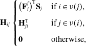 \begin{equation} \mathbf{H}_{ij}\begin{cases}{\left (\mathbf{F}_i^j\right )}^{\mathrm{T}}\mathbf{S}_j &\text{if } i\in \nu (j), \\[5pt] \mathbf{H}_{ji}^{\mathrm{T}} &\text{if } j\in \nu (i), \\[5pt] \mathbf{0} &\text{otherwise}, \end{cases} \end{equation}
where
 $\mathbf{F}$
is a matrix whose block-columns
$\mathbf{F}$
is a matrix whose block-columns
 $\mathbf{F}_i$
are the spatial forces required at the floating base to support unit accelerations about joint variable
$\mathbf{F}_i$
are the spatial forces required at the floating base to support unit accelerations about joint variable
 $i$
[Reference Featherstone1], with each of these block-columns being defined as:
$i$
[Reference Featherstone1], with each of these block-columns being defined as:
 \begin{equation} \mathbf{F}_i = \mathbf{I}_{\text{c}i}\mathbf{S}_i. \end{equation}
Finally, by applying the force transformation matrix to
 $\mathbf{F}_i$
we obtain
$\mathbf{F}_i$
we obtain
 $\mathbf{F}_i^j = \mathbf{\overline{X}}_i^j\mathbf{F}_i ={\left (\mathbf{X}_{j}^{i}\right )}^{\mathrm{T}}\mathbf{F}_i$
.
$\mathbf{F}_i^j = \mathbf{\overline{X}}_i^j\mathbf{F}_i ={\left (\mathbf{X}_{j}^{i}\right )}^{\mathrm{T}}\mathbf{F}_i$
.
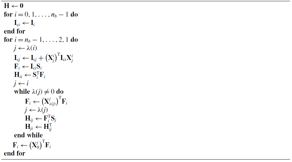
As can be seen in Algorithm 5, the outward pass involves storing the spatial inertia terms for each body, while the inward pass computes the resulting composite-rigid-body inertia and the joint-space inertia matrix.
Algorithm 5. Joint-space inertia
4.5. Joint-space equations of motion
With all its elements defined, the equations of motion can be formulated as:
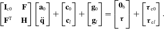 \begin{equation} \begin{bmatrix} \mathbf{I}_{\text{c}0} \;\;\;\; & \mathbf{F} \\[5pt] \mathbf{F}^{\text{T}} \;\;\;\; & \mathbf{H} \end{bmatrix} \begin{bmatrix} \mathbf{a}_0 \\[5pt] \ddot{\mathbf{q}} \end{bmatrix} + \begin{bmatrix} \mathbf{c}_0 \\[5pt] \mathbf{c}_l \end{bmatrix} + \begin{bmatrix} \mathbf{g}_0 \\[5pt] \mathbf{g}_l \end{bmatrix} = \begin{bmatrix} \mathbf{0}_6\\[5pt] \boldsymbol{\tau } \\[5pt] \end{bmatrix} + \begin{bmatrix} \boldsymbol{\tau }_{\text{e}0} \\[5pt] \boldsymbol{\tau }_{\text{e}l} \end{bmatrix}. \end{equation}
The first block-row portrays the dynamics of the trunk (floating base), with the second block-row characterizing the leg dynamics. By aggregating common terms as single matrices and vectors, the EoM can be expressed as:
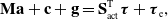 \begin{equation} \mathbf{M} \mathbf{a} + \mathbf{c} + \mathbf{g} = \mathbf{S}_{\text{act}}^{\text{T}} \boldsymbol{\tau } + \boldsymbol{\tau }_{\text{e}}, \end{equation}
where
 $\mathbf M$
,
$\mathbf M$
,
 $\mathbf{c}$
, and
$\mathbf{c}$
, and
 $\mathbf{g}$
represent the joint-space inertia matrix, quadratic velocity force vector, and gravitational force vector, respectively, and
$\mathbf{g}$
represent the joint-space inertia matrix, quadratic velocity force vector, and gravitational force vector, respectively, and
 $\boldsymbol{\tau }_{\text{e}}$
represents the joint-space external forces vector. Vector
$\boldsymbol{\tau }_{\text{e}}$
represents the joint-space external forces vector. Vector
 $\mathbf{a}$
represents the generalized acceleration vector which is composed of the trunk acceleration
$\mathbf{a}$
represents the generalized acceleration vector which is composed of the trunk acceleration
 $\mathbf{a}_0$
along with the leg joint acceleration
$\mathbf{a}_0$
along with the leg joint acceleration
 $\ddot{\mathbf{q}}$
, that is,
$\ddot{\mathbf{q}}$
, that is,
 $\mathbf{a} = (\mathbf{a}_0, \ddot{\mathbf{q}})$
.
$\mathbf{a} = (\mathbf{a}_0, \ddot{\mathbf{q}})$
.
5. Contact dynamics
Compliant contact dynamics is composed of two consecutive steps, contact detection and contact force generation. For contact detection, we use the sphere-to-plane distance
 $d_{ck}$
between the spherical shell (with radius
$d_{ck}$
between the spherical shell (with radius
 $r$
, centered at the foot frame origin) and the ground plane to check whether the foot is in contact, with
$r$
, centered at the foot frame origin) and the ground plane to check whether the foot is in contact, with
 $d_{ck}\leq 0$
implying there is contact between foot
$d_{ck}\leq 0$
implying there is contact between foot
 $k$
and the ground. As illustrated in Fig. 4, the sphere-to-plane distance
$k$
and the ground. As illustrated in Fig. 4, the sphere-to-plane distance
 $d_{ck}$
can be obtained by computing the signed distance
$d_{ck}$
can be obtained by computing the signed distance
 $d_{fk}$
between the ground plane and foot frame origin and subtracting the spherical shell radius. The signed distance
$d_{fk}$
between the ground plane and foot frame origin and subtracting the spherical shell radius. The signed distance
 $d_{fk}$
is computed as the projection of the foot position vector relative to point
$d_{fk}$
is computed as the projection of the foot position vector relative to point
 $P$
on the ground plane onto the surface normal (defined by the z-axis of the contact frame
$P$
on the ground plane onto the surface normal (defined by the z-axis of the contact frame
 $\hat{\boldsymbol{z}}_{C_k}^{W}$
), that is,
$\hat{\boldsymbol{z}}_{C_k}^{W}$
), that is,
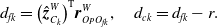 \begin{equation} d_{fk} ={\left (\hat{\boldsymbol{z}}_{C_k}^{W}\right )}^{\mathrm{T}}\boldsymbol{r}_{O_{P}O_{fk}}^{W}, \quad d_{ck} = d_{fk} - r. \end{equation}
We chose to model the ground as a horizontal plane, allowing point
 $P$
to be defined as the origin of the world frame and the ground plane orientation to be equal to the world frame, that is,
$P$
to be defined as the origin of the world frame and the ground plane orientation to be equal to the world frame, that is,
 $\mathbf{R}_{W}^{C_k} = \mathbf{R}_{C_k}^{W} = \mathbf{1}_3$
. Note that this procedure is also applicable when the ground plane is not horizontal.
$\mathbf{R}_{W}^{C_k} = \mathbf{R}_{C_k}^{W} = \mathbf{1}_3$
. Note that this procedure is also applicable when the ground plane is not horizontal.
Figure 4. Required components to compute the sphere-to-plane distance
 $d_{ck}$
used for contact detection.
$d_{ck}$
used for contact detection.
Given the point contact assumption, only the linear force element from the external wrench acting on each leg
 $k$
in contact is nonzero. This contact force is made up of three components, the normal component
$k$
in contact is nonzero. This contact force is made up of three components, the normal component
 $f_{\text{n}}$
which acts on the z-axis of the contact frame, and frictional components
$f_{\text{n}}$
which acts on the z-axis of the contact frame, and frictional components
 $f_{\text{t}x}$
and
$f_{\text{t}x}$
and
 $f_{\text{t}y}$
which act on the
$f_{\text{t}y}$
which act on the
 $x$
- and
$x$
- and
 $y$
-axis of the contact frame.
$y$
-axis of the contact frame.
Respective to leg
 $k$
, the contact frame
$k$
, the contact frame
 $\{C_k\}$
is located at the point on the foot that is closest to the ground plane. Each contact frame is equivalent to frame
$\{C_k\}$
is located at the point on the foot that is closest to the ground plane. Each contact frame is equivalent to frame
 $\{F_i\}$
in Algorithm 4, where
$\{F_i\}$
in Algorithm 4, where
 $i$
is the body respectively attached to foot
$i$
is the body respectively attached to foot
 $k$
(e.g.,
$k$
(e.g.,
 $i=3$
for
$i=3$
for
 $k=1$
). The force transformation matrix used to transform the contact wrench from
$k=1$
). The force transformation matrix used to transform the contact wrench from
 $\{C_k\}$
to
$\{C_k\}$
to
 $\{i\}$
is defined as:
$\{i\}$
is defined as:
 \begin{equation} \mathbf{\overline{X}}_{C_k}^i ={\left (\mathbf{X}_i^{C_k}\right )}^{\mathrm{T}} ={\left (\mathbf{X}_{fk}^{C_k}\mathbf{X}_{i}^{fk}\right )}^{\mathrm{T}}, \end{equation}
where
 $\mathbf{X}_i^{fk}$
is a known constant factor obtained from (16) and
$\mathbf{X}_i^{fk}$
is a known constant factor obtained from (16) and
 $\mathbf{X}_{fk}^{C_k}$
is the motion transformation matrix from the foot frame to the contact frame, which can be expressed as:
$\mathbf{X}_{fk}^{C_k}$
is the motion transformation matrix from the foot frame to the contact frame, which can be expressed as:
 \begin{equation} \mathbf{X}_{fk}^{C_k} = \begin{bmatrix} \mathbf{R}_{fk}^{C_k} \;\;\;\; & \mathbf{0}_{3 \times 3} \\[5pt] \tilde{\boldsymbol{r}}_{O_{C_k}O_{fk}}^{C_k}\mathbf{R}_{fk}^{C_k}\;\;\;\; & \mathbf{R}_{fk}^{C_k} \end{bmatrix},\quad \boldsymbol{r}_{O_{C_k}O_{fk}}^{C_k} = \begin{bmatrix} 0\\[5pt] 0\\[5pt] r \end{bmatrix}, \end{equation}
where
 $\mathbf{R}_{fk}^{C_k} ={\left (\mathbf{R}_{W}^{fk}\mathbf{R}_{C_k}^{W}\right )}^{\mathrm{T}}$
, with
$\mathbf{R}_{fk}^{C_k} ={\left (\mathbf{R}_{W}^{fk}\mathbf{R}_{C_k}^{W}\right )}^{\mathrm{T}}$
, with
 $\mathbf{R}_{W}^{fk}$
being the rotation matrix which can be extracted from (17) and
$\mathbf{R}_{W}^{fk}$
being the rotation matrix which can be extracted from (17) and
 $\mathbf{R}_{C_k}^{W}$
the rotation matrix which defines the ground plane orientation (in our case,
$\mathbf{R}_{C_k}^{W}$
the rotation matrix which defines the ground plane orientation (in our case,
 $\mathbf{R}_{C_k}^{W} = \mathbf{1}_3$
).
$\mathbf{R}_{C_k}^{W} = \mathbf{1}_3$
).
5.1. Normal contact force
The normal contact force
 $f_{\text{n}}$
results from the sum of an elastic and a damping term (
$f_{\text{n}}$
results from the sum of an elastic and a damping term (
 $f_{\text{n}} = f_{\text{s}} + f_{\text{d}}$
). The elastic term
$f_{\text{n}} = f_{\text{s}} + f_{\text{d}}$
). The elastic term
 $f_{\text{s}}$
is computed using a nonlinear Hertz model, that is,
$f_{\text{s}}$
is computed using a nonlinear Hertz model, that is,
 \begin{equation} f_{\text{s}} = -K \delta ^e, \end{equation}
where
 $K$
is the stiffness,
$K$
is the stiffness,
 $\delta =d_{ck}$
is the ground penetration, and
$\delta =d_{ck}$
is the ground penetration, and
 $e$
is the force exponent. The damping term
$e$
is the force exponent. The damping term
 $f_{\text{d}}$
can be expressed as:
$f_{\text{d}}$
can be expressed as:
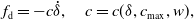 \begin{equation} f_{\text{d}} = -c\dot{\delta },\quad c = c(\delta, c_{\text{max}}, w), \end{equation}
where
 $\dot{\delta }$
is the ground penetration rate,
$\dot{\delta }$
is the ground penetration rate,
 $c$
is the effective damping coefficient,
$c$
is the effective damping coefficient,
 $c_{\text{max}}$
is the nominal damping coefficient, and
$c_{\text{max}}$
is the nominal damping coefficient, and
 $w$
is the ramp-up distance. An effective damping coefficient is used to avoid the natural discontinuity on impact. This term is computed through a smoothstep function used to ramp up the damping coefficient from 0 to
$w$
is the ramp-up distance. An effective damping coefficient is used to avoid the natural discontinuity on impact. This term is computed through a smoothstep function used to ramp up the damping coefficient from 0 to
 $c_{\text{max}}$
over the range
$c_{\text{max}}$
over the range
 $\delta \in [\!-\!w, 0]$
.
$\delta \in [\!-\!w, 0]$
.
As a result of taking the derivative of (31), the ground penetration rate
 $\dot{\delta }$
is found to be equivalent to the foot linear velocity component in the z-axis of the contact frame, that is,
$\dot{\delta }$
is found to be equivalent to the foot linear velocity component in the z-axis of the contact frame, that is,
 \begin{equation} \dot{\delta } ={\left (\hat{\boldsymbol{z}}_{C_k}^W\right )}^{\mathrm{T}}\boldsymbol{v}_{fk}^{W}. \end{equation}
Note that
 $\boldsymbol{v}_{fk}^{W}$
is the linear velocity component of the spatial velocity vector
$\boldsymbol{v}_{fk}^{W}$
is the linear velocity component of the spatial velocity vector
 $\mathbf{v}_{fk}^{W} = (\boldsymbol{\omega }_{fk}^{W}, \boldsymbol{v}_{fk}^{W})$
, which can be computed from the spatial velocity of the last link
$\mathbf{v}_{fk}^{W} = (\boldsymbol{\omega }_{fk}^{W}, \boldsymbol{v}_{fk}^{W})$
, which can be computed from the spatial velocity of the last link
 $i$
of leg
$i$
of leg
 $k$
such that
$k$
such that
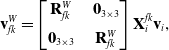 \begin{equation} \mathbf{v}_{fk}^{W} = \begin{bmatrix} \mathbf{R}_{fk}^{W} \;\;\;\; & \mathbf{0}_{3 \times 3} \\[5pt] \mathbf{0}_{3 \times 3} \;\;\;\; & \mathbf{R}_{fk}^{W} \end{bmatrix}\mathbf{X}_i^{fk}\mathbf{v}_{i}, \end{equation}
where
 $\mathbf{X}_i^{fk}$
is a known constant factor (16) and
$\mathbf{X}_i^{fk}$
is a known constant factor (16) and
 $\mathbf{R}_{fk}^{W}$
is obtained from the inverse of (17).
$\mathbf{R}_{fk}^{W}$
is obtained from the inverse of (17).
5.2. Friction contact force
The frictional components
 $f_x$
and
$f_x$
and
 $f_y$
of the contact force are computed using a Coulomb friction model such that
$f_y$
of the contact force are computed using a Coulomb friction model such that
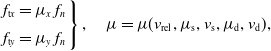 \begin{equation} \left .\begin{array}{c} f_{\text{t}x} = \mu _x \;f_n\\[5pt] f_{\text{t}y} = \mu _y \;f_n \end{array}\right \},\quad \mu = \mu (v_{\text{rel}}, \mu _{\text{s}}, v_{\text{s}}, \mu _{\text{d}}, v_{\text{d}}), \end{equation}
where
 $\mu$
is the effective friction coefficient,
$\mu$
is the effective friction coefficient,
 $v_{\text{rel}}$
is the relative velocity (either
$v_{\text{rel}}$
is the relative velocity (either
 $x$
or
$x$
or
 $y$
component of
$y$
component of
 $\boldsymbol{v}_{C_k}$
, the linear component of the contact frame velocity defined as
$\boldsymbol{v}_{C_k}$
, the linear component of the contact frame velocity defined as
 $\mathbf{v}_{C_k} = \mathbf{X}_i^{C_k}\mathbf{v}_{i}$
),
$\mathbf{v}_{C_k} = \mathbf{X}_i^{C_k}\mathbf{v}_{i}$
),
 $\mu _{\text{d}}$
is the dynamic friction coefficient,
$\mu _{\text{d}}$
is the dynamic friction coefficient,
 $v_{\text{d}}$
is the stiction-sliding transition velocity,
$v_{\text{d}}$
is the stiction-sliding transition velocity,
 $\mu _{\text{s}}$
is the static friction coefficient, and
$\mu _{\text{s}}$
is the static friction coefficient, and
 $v_{\text{s}}$
is the velocity where
$v_{\text{s}}$
is the velocity where
 $\mu =\mu _{\text{s}}$
. The effective friction coefficient is computed through a smoothstep function used to transition from the negative to the positive static friction coefficient (which occurs when the relative velocity sense is reversed) and from the static to the sliding friction coefficient.
$\mu =\mu _{\text{s}}$
. The effective friction coefficient is computed through a smoothstep function used to transition from the negative to the positive static friction coefficient (which occurs when the relative velocity sense is reversed) and from the static to the sliding friction coefficient.
6. Simulation setup
To evaluate the proposed method, the algorithms were implemented in Simulink using a Level-2 MATLAB S-Function block. Although the algorithms do not imply any specific coding language, Simulink was used due to the authors’ familiarity with the tool. Given that it can model continuous state behavior including state dynamics, the MATLAB S-Function block is the preferred method to implement continuous-time dynamic systems, such as our rigid-body mechanical system, within Simulink.
6.1. State-space formulation
Implementing the system in Simulink required a state-space representation of the EoM. Let
 $\mathbf{x}$
be the state vector such that
$\mathbf{x}$
be the state vector such that
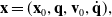 \begin{equation} \mathbf{x} = ( \mathbf{x}_0, \mathbf{q}, \mathbf{v}_0, \dot{\mathbf{q}}), \end{equation}
where
 $\mathbf{x}_0$
are the spatial coordinates (orientation and position) of the trunk,
$\mathbf{x}_0$
are the spatial coordinates (orientation and position) of the trunk,
 $\mathbf{q}$
are the leg joint angles,
$\mathbf{q}$
are the leg joint angles,
 $\mathbf{v}_0$
is the spatial velocity (angular and linear velocity) of the trunk, and
$\mathbf{v}_0$
is the spatial velocity (angular and linear velocity) of the trunk, and
 $\dot{\mathbf{q}}$
are the leg joint velocities. The state vector time derivative is defined as:
$\dot{\mathbf{q}}$
are the leg joint velocities. The state vector time derivative is defined as:
 \begin{equation} \dot{\mathbf{x}} = (\dot{\mathbf{x}}_0, \dot{\mathbf{q}}, \mathbf{a}_0,\ddot{\mathbf{q}}). \end{equation}
Note that the derivative of the orientation is not equivalent to the angular velocity, that is,
 $\dot{\mathbf{x}}_0 \neq \mathbf{v}_0$
. Given that the state derivative must be a function of the inputs, of the states, and possibly of time, this must be addressed by performing a conversion from angular velocity (which is part of the state vector) to Euler Angle rate. For a body-fixed ZYX Euler Angle sequence
$\dot{\mathbf{x}}_0 \neq \mathbf{v}_0$
. Given that the state derivative must be a function of the inputs, of the states, and possibly of time, this must be addressed by performing a conversion from angular velocity (which is part of the state vector) to Euler Angle rate. For a body-fixed ZYX Euler Angle sequence
 $\boldsymbol{\xi } = (\psi, \theta, \phi )$
, the conversion matrix
$\boldsymbol{\xi } = (\psi, \theta, \phi )$
, the conversion matrix
 $\mathbf{G}$
from Euler Angle rate
$\mathbf{G}$
from Euler Angle rate
 $\boldsymbol{\dot{\xi }}$
to angular velocity
$\boldsymbol{\dot{\xi }}$
to angular velocity
 $\boldsymbol{\omega }_0$
is formulated as:
$\boldsymbol{\omega }_0$
is formulated as:
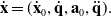
 \begin{equation} \mathbf{G} = \begin{bmatrix} 0 \;\;\;\; & -\sin\!(\psi )\;\;\;\; & \cos\!(\theta )\cos\!(\psi ) \\[5pt] 0\;\;\;\; & \cos\!(\psi )\;\;\;\; & \cos\!(\theta )\sin\!(\psi ) \\[5pt] 1\;\;\;\; & 0\;\;\;\; & -\sin\!(\theta ) \end{bmatrix},\quad \boldsymbol{\omega }_0 = \mathbf{G}\boldsymbol{\dot{\xi }}. \end{equation}
Taking the inverse of this conversion matrix,
 $\dot{\mathbf{x}}_0$
can be expressed as a function of
$\dot{\mathbf{x}}_0$
can be expressed as a function of
 $\mathbf{v}_0$
such that
$\mathbf{v}_0$
such that
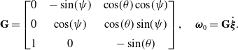
 \begin{equation} \dot{\mathbf{x}}_0 = \mathbf{T}\mathbf{v}_0,\quad \mathbf{T} = \begin{bmatrix} \mathbf{G}^{\mathrm{-1}}\;\;\;\; & \mathbf{0}_{3\times 3} \\[5pt] \mathbf{0}_{3\times 3}\;\;\;\; & \mathbf{1}_3 \end{bmatrix}. \end{equation}
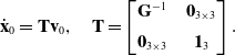
With the state vector and its first time derivative defined, by substituting the EoM (30) into the last two block-rows of (40), the state-space equations of the system can be expressed as:
 \begin{equation} \dot{\mathbf{x}} = \begin{bmatrix} \mathbf{T}\mathbf{v}_0 \\[5pt] \ddot{\mathbf{q}}\\[5pt] \mathbf{M}^{\mathrm{-1}}\left (\mathbf{S}_{\text{act}}^{\mathrm{T}}\boldsymbol{\tau }+\boldsymbol{\tau }_{\text{e}}-(\mathbf{c}+\mathbf{g})\right ) \end{bmatrix}. \end{equation}
6.2. Locomotion control
To make the quadruped robot move, a foot trajectory was established and a control scheme to track it was defined. The former was implemented using a foot trajectory generator defined in our previous work [Reference De Paula, Godoy and Becerra-Vargas20], while the latter was defined to be a PD-independent joint controller for each leg implemented using a MATLAB Function block. The foot trajectory generator is comprised of a Central Pattern Generator to synthesize rhythmic signals matching a quadruped gait (in this case, the trot gait) that drive Bézier curves respective to the two stages of locomotion (i.e., stance and swing phase). Given that the resulting curves are planar, inverse kinematics was used to compute the hip and knee joint angles, with the abduction/adduction joints always set to 0. Regarding control, for active joint
 $i$
, its control law can be expressed as:
$i$
, its control law can be expressed as:
 \begin{equation} \tau _i = k_{\text{p}}(q_i-q_{\text{d}i})+k_{\text{d}}\dot{q}_i. \end{equation}
where
 $k_{\text{p}}$
is the proportional gain,
$k_{\text{p}}$
is the proportional gain,
 $k_{\text{d}}$
is the derivative gain,
$k_{\text{d}}$
is the derivative gain,
 $q_i$
is the measured joint angle,
$q_i$
is the measured joint angle,
 $q_{\text{d}i}$
is the desired joint angle computed from the inverse kinematics of the leg trajectory, and
$q_{\text{d}i}$
is the desired joint angle computed from the inverse kinematics of the leg trajectory, and
 $\dot{q}_i$
is the measured joint velocity. Note that the derivative component was added as a feedforward term to increase stability.
$\dot{q}_i$
is the measured joint velocity. Note that the derivative component was added as a feedforward term to increase stability.
6.3. Baseline behavior
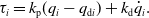
A comparative analysis with same robot implemented using the readily available physics engine MuJoCo [Reference Todorov, Erez and Tassa18] was performed to evaluate the implementation of the algorithms. While the quadruped robot model was the same in both software, the contact model was not. Unlike the compliant method described in Section 5, MuJoCo uses an augmented non-smooth method that models contact as geometric constraints with an added regularization term. Even though different methods were used to model the contact dynamics, this analysis serves as a way to show if the system behavior was at least similar. Table I summarizes the simulation parameters used for our simulator and MuJoCo, including the integration method, time step, simulation time, contact parameters, and controller gains. Note that both approaches use a three-component contact dimension (point contact) and have an elliptic friction cone shape.
Table I. Simulation parameters used for our simulator and the MuJoCo physics engine.
 $^{\dagger}\!$
For MuJoCo, stiffness and damping terms have a distinct meaning from those defined for our simulator’s contact model. MuJoCo employs these parameters alongside an impedance parameter [Reference Todorov, Erez and Tassa18] to compute the regularization term used to incorporate the geometric constraints that model the contact dynamics.
$^{\dagger}\!$
For MuJoCo, stiffness and damping terms have a distinct meaning from those defined for our simulator’s contact model. MuJoCo employs these parameters alongside an impedance parameter [Reference Todorov, Erez and Tassa18] to compute the regularization term used to incorporate the geometric constraints that model the contact dynamics.
Since the simulation is composed of the robot and the contact dynamics, aspects related to each of these elements were analyzed. The trunk pose was used to represent the robot behavior as its observed state reflects the states from all the legs and their interaction with the ground. Regarding the contact dynamics, contact activation, a binary signal where 1 (one) indicates when contact forces are nonzero, and the measured ground reaction forces from a single leg were used. To quantify the disparity between MuJoCo and our simulator, both the respective time series and mean absolute error of each scalar component were used.
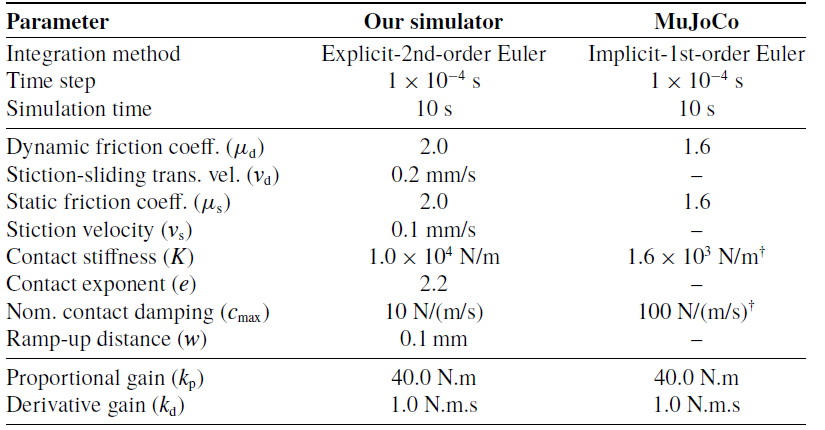
7. Results
Figure 5 shows the trunk’s position and orientation obtained in simulation. Very similar trunk pose was observed in both simulators, registering (63, 17, 4.6) mm mean absolute error for the position components and (1.5, 1.3, 2.7) deg for the Euler Angles. Despite using the same robot and controller, the trunk pose was not expected to be a perfect match due to the distinct methods used to model the contact dynamics, which affect how contact force generation is performed and, consequently, how a particular motion evolves in time.
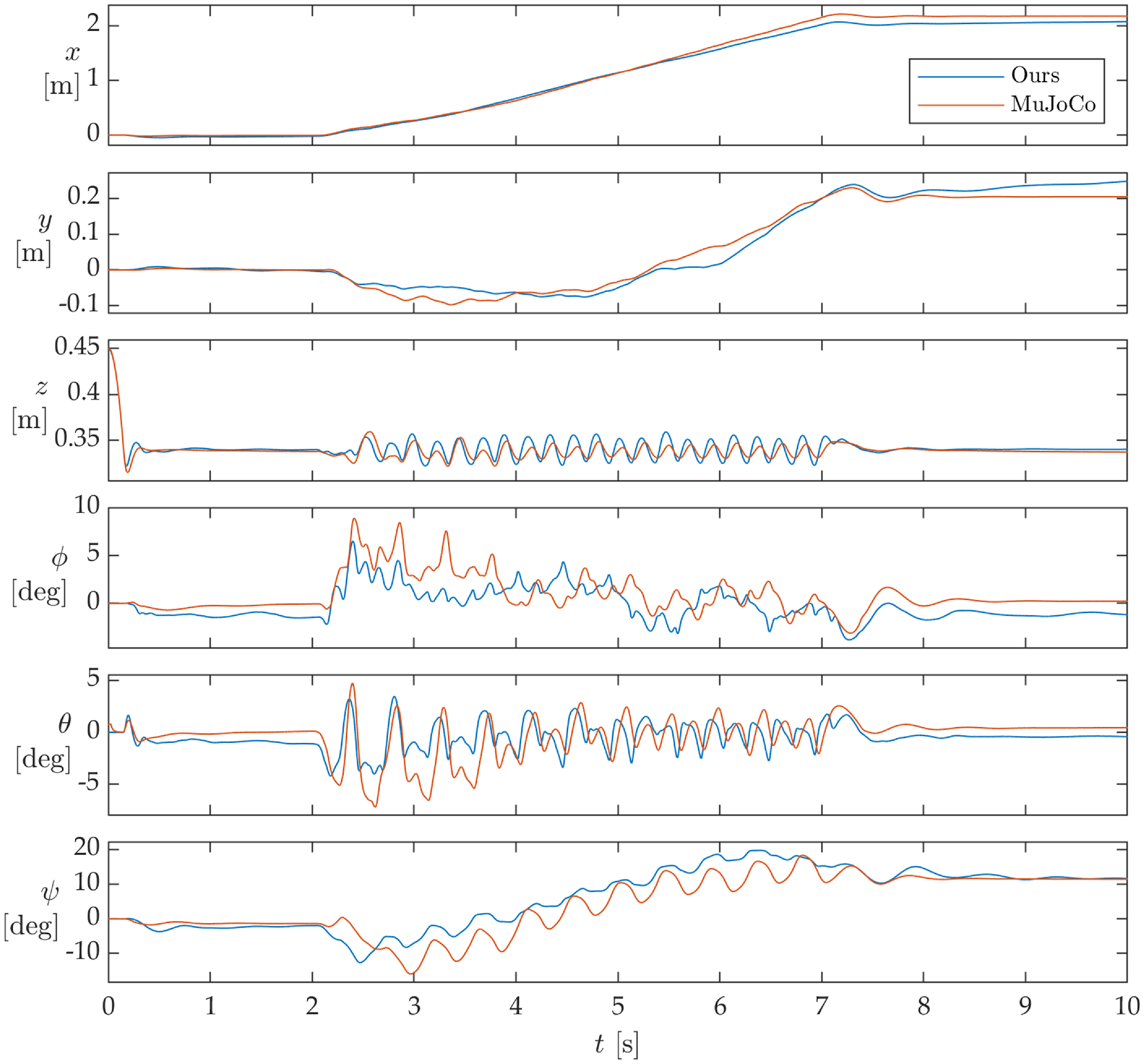
Figure 5. Quadruped robot trunk position and orientation obtained in simulation.
Figure 6. Contact activation and vertical contact forces applied to the left foreleg obtained in simulation.
Figure 6 shows the left forelimb’s contact activation and the vertical (normal) ground reaction force. Very similar activation time was observed, with MuJoCo having a few spurious impulsive signals at 2.8, 4.6, 5.0, 5.9, and 6.4 s. Regarding the ground reaction forces, our approach resulted in slightly higher peak values, yielding a mean absolute contact force error of 5.65 N. The higher peak values can be traced to the higher effective contact stiffness and lower damping defined for our contact model. Note that in MuJoCo, the stiffness and damping terms presented in Table I are used to compute a reference acceleration term, which is only a single component of the cost function that is optimized to generate the constraint forces and update the joint acceleration while accounting for the constraints. Also, with regard to processing time, simulating 10 s took 300 s using our implementation, while it took only 20 s with MuJoCo. This order of magnitude discrepancy can have a multitude of reasons, from the intrinsic overhead of the Level-2 MATLAB S-Function to the limitations of the contact dynamics method when using a high stiffness coefficient. Since simulation speed (though always desirable) was not a critical feature for this work, we restricted ourselves to only noting the issue here until we can address it in future works.
8. Conclusion
In this paper, we characterized the quadruped robot and contact dynamics that will compose our in-house simulator. The robot dynamics was derived using the RNEA and CRBA, ensuring each component of the bias term was explicit to allow for ease of usage in control systems. Contact dynamics was modeled using a compliant method composed of a nonlinear spring-damper model for the normal component and a smooth stick-slip model for the friction components. We used a simple PD-independent joint controller to track a desired leg trajectory and allow for the robot locomotion to be evaluated. When comparing the characteristic locomotion signals with the same robot and controller implemented using MuJoCo, we observed similar behavior for both simulators despite the significantly different contact models. Though activation timing was a very close match, the distinct methods used to generate the contact forces ended up causing differences in the contact forces and the resulting trunk pose. Despite our implementation being an order of magnitude slower than MuJoCo, the fact that it resulted in similar behavior shows that the underlying mechanics were sound, allowing for the next steps to be focused on improving aspects such as simulation speed. Future works can try to optimize the existing implementation to increase computational speed while maintaining an acceptable level of accuracy, making it applicable for both rapid prototyping and real-time legged robot control.
Author contributions
Conceptualization, provision of resources, software development, and data collection were carried out by Mauricio Becerra-Vargas. Data curation and analysis, visualization, and manuscript revision were performed by Daniel Teixeira de Paula. Supervision and project administration were done by Eduardo Paciencia Godoy. All authors have read and approved the final manuscript.
Financial support
This research received no specific grant from any funding agency, commercial, or not-for-profit sectors.
Competing interests
The authors declare no conflicts of interest exist.
Ethical approval
None.
Appendix
A. Definitions
A.1. Skew-symmetric matrix
Let
 $\boldsymbol{v}$
be a vector with components
$\boldsymbol{v}$
be a vector with components
 $v_1, v_2$
, and
$v_1, v_2$
, and
 $v_3$
. The skew-symmetric matrix
$v_3$
. The skew-symmetric matrix
 $\tilde{\boldsymbol{v}}$
is defined as:
$\tilde{\boldsymbol{v}}$
is defined as:
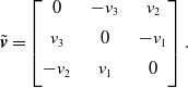 \begin{equation} \tilde{\boldsymbol{v}} = \begin{bmatrix} 0\;\;\;\; & -v_3\;\;\;\; & v_2\\[5pt] v_3\;\;\;\; & 0\;\;\;\; & -v_1\\[5pt] -v_2\;\;\;\; & v_1\;\;\;\; & 0\\[5pt] \end{bmatrix}. \end{equation}
A.2. Twist cross product
Given the spatial velocity
 $\mathbf{v}=(\boldsymbol{\omega }, \boldsymbol{v})$
composed of the angular velocity
$\mathbf{v}=(\boldsymbol{\omega }, \boldsymbol{v})$
composed of the angular velocity
 $\boldsymbol{\omega }$
and linear velocity
$\boldsymbol{\omega }$
and linear velocity
 $\boldsymbol{v}$
, the twist cross-product operator
$\boldsymbol{v}$
, the twist cross-product operator
 $\mathbf{v}\ast$
can be defined as:
$\mathbf{v}\ast$
can be defined as:
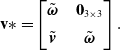 \begin{equation} \mathbf{v}\ast = \begin{bmatrix} \tilde{\boldsymbol{\omega }}\;\;\;\; & \mathbf{0}_{3 \times 3} \\[5pt] \tilde{\boldsymbol{v}}\;\;\;\; & \tilde{\boldsymbol{\omega }} \end{bmatrix}. \end{equation}
A.3. Wrench cross product
Given the spatial force
 $\mathbf{f}=(\boldsymbol{n}, \boldsymbol{f})$
composed of the couple moment
$\mathbf{f}=(\boldsymbol{n}, \boldsymbol{f})$
composed of the couple moment
 $\boldsymbol{n}$
and linear force
$\boldsymbol{n}$
and linear force
 $\boldsymbol{f}$
, the wrench cross-product operator
$\boldsymbol{f}$
, the wrench cross-product operator
 $\mathbf{f}\circledast$
can be defined as:
$\mathbf{f}\circledast$
can be defined as:
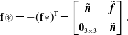 \begin{equation} \mathbf{f}\circledast = -(\mathbf{f}\!\ast\!)^{\mathrm{T}} = \begin{bmatrix} \tilde{\boldsymbol{n}}\;\;\;\; & \tilde{\boldsymbol{f}} \\[5pt] \mathbf{0}_{3 \times 3}\;\;\;\; & \tilde{\boldsymbol{n}} \end{bmatrix}. \end{equation}
B. Jacobian matrix computation
Let the geometric Jacobian matrix of the feet
 $\mathbf{J}_{\text{feet}}$
be a map from the joint velocities
$\mathbf{J}_{\text{feet}}$
be a map from the joint velocities
 $\mathbf{w} = (\mathbf{v}_0,\dot{\mathbf{q}})$
to the feet frame velocities
$\mathbf{w} = (\mathbf{v}_0,\dot{\mathbf{q}})$
to the feet frame velocities
 $\mathbf{v}_{\text{feet}}$
, such that
$\mathbf{v}_{\text{feet}}$
, such that
 $\mathbf{v}_{\text{feet}} = \mathbf{J}_{\text{feet}}\mathbf{w}$
, and let its transpose be a map from the forces applied to the foot frames
$\mathbf{v}_{\text{feet}} = \mathbf{J}_{\text{feet}}\mathbf{w}$
, and let its transpose be a map from the forces applied to the foot frames
 $\mathbf{f}_{\text{feet}}$
to the joint-space torques
$\mathbf{f}_{\text{feet}}$
to the joint-space torques
 $\boldsymbol{\tau }_{\text{e}}$
, such that
$\boldsymbol{\tau }_{\text{e}}$
, such that
 $\boldsymbol{\tau }_{\text{e}} ={\mathbf{J}_{\text{feet}}}^{\mathrm{T}}\mathbf{f}_{\text{feet}}$
. For
$\boldsymbol{\tau }_{\text{e}} ={\mathbf{J}_{\text{feet}}}^{\mathrm{T}}\mathbf{f}_{\text{feet}}$
. For
 $n_{\text{J}}$
joints and
$n_{\text{J}}$
joints and
 $m$
feet, the geometric Jacobian matrix of the feet
$m$
feet, the geometric Jacobian matrix of the feet
 $\mathbf{J}_{\text{feet}}$
is defined as:
$\mathbf{J}_{\text{feet}}$
is defined as:
 \begin{equation} \mathbf{J}_{\text{feet}} = \begin{bmatrix} \mathbf{J}_{\text{feet}, 1} \\[5pt] \vdots \\[5pt] \mathbf{J}_{\text{feet}, k} \\[5pt] \vdots \\[5pt] \mathbf{J}_{\text{feet}, m} \end{bmatrix},\quad \mathbf{J}_{\text{feet}, k} = \begin{bmatrix} \mathbf{J}_{\text{feet}, k1}\;\;\;\; & \cdots\;\;\;\; & \mathbf{J}_{\text{feet}, kn_{\text{J}}} \end{bmatrix}, \quad k\in [1, m], \end{equation}
where each block-row
 $\mathbf{J}_{\text{feet}, k}$
is associated with the spatial velocity
$\mathbf{J}_{\text{feet}, k}$
is associated with the spatial velocity
 $\mathbf{v}_{fk}$
of foot
$\mathbf{v}_{fk}$
of foot
 $k$
such that
$k$
such that
 $\mathbf{v}_{fk} = \mathbf{J}_{\text{feet}, k}\mathbf{w}$
. Given that each foot is attached to a specific body in the kinematic tree, we define a feet index array
$\mathbf{v}_{fk} = \mathbf{J}_{\text{feet}, k}\mathbf{w}$
. Given that each foot is attached to a specific body in the kinematic tree, we define a feet index array
 $\varphi$
that stores the bodies correspondent to each foot, where
$\varphi$
that stores the bodies correspondent to each foot, where
 $\varphi (k)$
is the body index respective to foot
$\varphi (k)$
is the body index respective to foot
 $k$
.
$k$
.
The spatial velocity
 $\mathbf{v}_{fk}$
can be computed from the spatial velocity of its attached body
$\mathbf{v}_{fk}$
can be computed from the spatial velocity of its attached body
 $\mathbf{v}_{i}$
, where
$\mathbf{v}_{i}$
, where
 $i = \varphi (k)$
, which can be expressed as a function of the joint velocities, that is,
$i = \varphi (k)$
, which can be expressed as a function of the joint velocities, that is,
 \begin{equation} \mathbf{v}_{fk} = \mathbf{X}^{fk}_i\mathbf{v}_{i} = \mathbf{X}^{fk}_i\sum _{j\in \kappa (i)}\mathbf{X}^i_j \mathbf{S}_j \dot{\mathbf{q}}_j, \end{equation}
where
 $\kappa (i)$
is the support set of body
$\kappa (i)$
is the support set of body
 $i$
(which contains all the joints between body
$i$
(which contains all the joints between body
 $i$
and the root node, in this case the ground). Note that index
$i$
and the root node, in this case the ground). Note that index
 $j$
is not necessarily
$j$
is not necessarily
 $\lambda (i)$
; therefore, not all motion transformation matrices will be available from the standard kinematics loop presented in Algorithm 1. Here, we assume that the necessary modifications were done and that all motion transformation matrices are available.
$\lambda (i)$
; therefore, not all motion transformation matrices will be available from the standard kinematics loop presented in Algorithm 1. Here, we assume that the necessary modifications were done and that all motion transformation matrices are available.
From (B2), we can infer that each term multiplying a joint velocity
 $\dot{\mathbf{q}}_j$
is equivalent to a block-column
$\dot{\mathbf{q}}_j$
is equivalent to a block-column
 $\mathbf{J}_{\text{feet}, kj}$
of (B1), that is,
$\mathbf{J}_{\text{feet}, kj}$
of (B1), that is,
 \begin{equation} \mathbf{J}_{\text{feet}, kj} = \mathbf{X}^{fk}_i \left (\mathbf{X}^i_j \mathbf{S}_j\right ). \end{equation}
This expression suggests that we can compute the Jacobian matrix by traversing the support path defined for each foot as presented in Algorithm 6. Note that the first transform
 $\mathbf{X}^{fk}_i$
is applied only once per foot to the entire block-row matrix
$\mathbf{X}^{fk}_i$
is applied only once per foot to the entire block-row matrix
 $\mathbf{J}_{\text{feet}, k}$
. If the measured contact forces or the desired spatial velocities are expressed in the contact frame
$\mathbf{J}_{\text{feet}, k}$
. If the measured contact forces or the desired spatial velocities are expressed in the contact frame
 $\{C_k\}$
, transform
$\{C_k\}$
, transform
 $\mathbf{X}_{fk}^{C_k}$
defined in (33) can be pre-multiplied to (B3).
$\mathbf{X}_{fk}^{C_k}$
defined in (33) can be pre-multiplied to (B3).
Algorithm 6. Jacobian computation