4.1. Solution for potential function $\varphi$

Considering the derivative relationship between gas-phase velocity and the scalar potential $\varphi$, as described in (2.4), we can, without compromising the generality of the solution, set the value of $\varphi$ to zero at infinity, i.e. $\varphi (\xi = 0, \theta = 0) = 0$. When $\varphi$ maintains constant values, $\varphi _{s,1}$ and $\varphi _{s,2}$, on the surfaces of two droplets, defined at $\xi = \xi _1$ and $\xi = \xi _2$, respectively, the Laplace equation of $\varphi$, given by (2.10), can be solved using the separation of variables method (Morse & Feshbach Reference Morse and Feshbach1954). This approach yields the exact solution for $\varphi$ in the form of an infinite series as

(4.1)\begin{align} \varphi &= \sqrt{ 2(\cosh \xi - \cos \theta) } \sum_{n=0}^\infty \left[ \frac{( \varphi_{s,1} \,\mathrm{e}^{(2n+1)\xi_1} - \varphi_{s,2} )}{\mathrm{e}^{(2n+1)\xi_1} - \mathrm{e}^{(2n+1)\xi_2}} \,\mathrm{e}^{(n + 1/2) \xi}\right.\nonumber\\ &\quad\left. {}+ \frac{\mathrm{e}^{(2n+1)\xi_1}\,( \varphi_{s,2} - \varphi_{s,1} \,\mathrm{e}^{(2n+1)\xi_2} ) }{ \mathrm{e}^{(2n+1)\xi_1} - \mathrm{e}^{(2n+1)\xi_2} } \,\mathrm{e}^{-(n + 1/2) \xi} \right] P_n (\cos \theta), \end{align}

where $P_n (\cdot )$ represents the $n$th-order Legendre polynomial.

Because the mass flux at the droplet surface is affected by the local gradient of the fuel vapour mass fraction, the values of $\varphi _{s,i}$ have not yet been determined. In fact, even the uniformity of $\varphi _{s,i}$ across the surfaces of the droplets cannot be ensured. To address this, it is necessary to incorporate the convection–diffusion equation of the coupling function $\beta _k$, as specified in (2.11). The corresponding boundary conditions on both droplet surfaces should be applied to derive coupled solutions for $\varphi$ and $\beta _k$.

4.2. Solution for coupling function $\beta _{FO}$

Considering the boundary conditions for $T_g$, $Y_F$ and $Y_O$ at the surfaces of both droplets and at infinity, the boundary conditions for the three coupling functions, as defined in (2.2), read

(4.2)\begin{equation} \left.\begin{array}{@{}c@{}} \beta_{FO,s,1} = \dfrac{Y_{F,s,1} }{ W_F \nu_F }, \quad \beta_{TF,s,1} = \dfrac{c_{p,g} T_{s,1} }{ q_c } + \dfrac{Y_{F,s,1} }{ W_F \nu_F }, \quad \beta_{TO,s,1} = \dfrac{c_{p,g} T_{s,1} }{ q_c }, \\[10pt] \beta_{FO,s,2} = \dfrac{Y_{F,s,2} }{ W_F \nu_F }, \quad \beta_{TF,s,2} = \dfrac{c_{p,g} T_{s,2} }{ q_c } + \dfrac{Y_{F,s,2} }{ W_F \nu_F }, \quad \beta_{TO,s,2} = \dfrac{c_{p,g} T_{s,2} }{ q_c }, \\[10pt] \beta_{FO,\infty} ={-} \dfrac{Y_{O,\infty} }{ W_O \nu_O }, \quad \beta_{TF,\infty} = \dfrac{c_{p,g} T_\infty }{ q_c }, \quad \beta_{TO,\infty} = \dfrac{c_{p,g} T_\infty }{ q_c } + \dfrac{Y_{O,\infty} }{ W_O \nu_O }. \end{array}\right\} \end{equation}

One possible solution for $\beta _k$ to (2.6) can be represented in the form

(4.3a,b)\begin{equation} \beta_k = A_k + B_k \times \mathcal{L} (\varphi), \quad \mathcal{L} (\varphi) \equiv \exp \left[ - \frac{\varphi }{ (\rho_g D)_\infty } \right], \end{equation}

where $A_k$ and $B_k$ are undetermined coefficients. This form of solution indicates that $\beta _k$ is a one-dimensional function of $\varphi$. Since (4.3) contains only two undetermined coefficients, while there are three boundary conditions to satisfy (see (4.2)), the validity of this general solution hinges on the existence of a specific relationship among these three boundary conditions.

Given that only fuel vapour exhibits mass flux at the surfaces of the droplets, i.e.

(4.4)\begin{equation} \left.\begin{array}{@{}c@{}} \dot{m}_{F,s,i} = \boldsymbol{n} \boldsymbol{\cdot} ( \rho_g \boldsymbol{v} Y_F - (\rho_g D)_\infty\,\boldsymbol{\nabla} Y_F )_{s,i} = ( \rho_g \boldsymbol{v})_{s,i},\\[3pt] \dot{m}_{O,s,i} = \boldsymbol{n} \boldsymbol{\cdot} ( \rho_g \boldsymbol{v} Y_O - (\rho_g D)_\infty\,\boldsymbol{\nabla} Y_O )_{s,i} = 0, \end{array}\right\} \end{equation}

where $\boldsymbol {n}$ represents the unit normal vector on the droplet surface. Considering (2.12) and (4.4), we have

(4.5a,b)\begin{equation} \left. (\rho_g D)_\infty\,\frac{\mathrm{d} Y_F}{\mathrm{d} \varphi} \right|_{s,i} = 1 - Y_{F,s,i}, \quad \left. {-(\rho_g D)_\infty}\,\frac{\mathrm{d} Y_O}{\mathrm{d} \varphi} \right|_{s,i} = Y_{O,s,i} = 0. \end{equation}

Then by using the relation between $\beta _{FO}$ and $Y_j$, we obtain

(4.6)\begin{equation} \left. \frac{\mathrm{d} \beta_{FO}}{\mathrm{d} \varphi} \right|_{s,i} = \frac{1 }{ (\rho_g D)_\infty }\,\frac{1 - Y_{F,s,i} }{ W_F \nu_F }. \end{equation}

Alternatively, if $\beta _{FO}$ adheres to the solution form provided in (4.3), based on the boundary conditions of $\beta _{FO}$ as outlined in (4.2), then we deduce that

(4.7)\begin{equation} \left. \frac{\mathrm{d} \beta_{FO}}{\mathrm{d} \varphi} \right|_{s,i} ={-} \frac{1 }{ (\rho_g D)_\infty } \left( \frac{Y_{O,\infty} }{ W_O \nu_O } + \frac{Y_{F,s,1} }{ W_F \nu_F } \right) \frac{\mathcal{L} (\varphi_{s,i}) }{ \mathcal{L} (\varphi_{s,1}) - 1 }. \end{equation}

Combining (4.6) and (4.7), we obtain

(4.8)\begin{equation} \frac{1 - Y_{F,s,i} }{ W_F \nu_F } ={-} \left( \frac{Y_{O,\infty} }{ W_O \nu_O } + \frac{Y_{F,s,1} }{ W_F \nu_F } \right) \frac{\mathcal{L} (\varphi_{s,i}) }{ \mathcal{L} (\varphi_{s,1}) - 1 }, \end{equation}

which is the relation that must be satisfied on the surfaces of both droplets. Further combining the expression of $\mathcal {L} (\varphi )$ from (4.3), the values of $\varphi$ on the droplet surfaces can be derived as

(4.9)\begin{equation} \varphi_{s,i} = (\rho_g D)_\infty \ln ( 1 + B_{v,i} ), \end{equation}

where $\varphi _{s,i}$ and $B_{v,i}$ represent the evaporation potential and Spalding transfer number of droplet $i$, respectively, and $B_{v,i}$ is defined as

(4.10)\begin{equation} B_{v,i} = \frac{Y_{F,s,i} + \phi Y_{O,\infty} }{ 1 - Y_{F,s,i} }, \quad \phi \equiv \frac{W_F \nu_F }{ W_O \nu_O }, \end{equation}

where $\phi$ is the fuel-to-oxygen mass stoichiometric ratio. According to (4.10), $B_{v,i}$ is a function of $\phi Y_{O,\infty }$ and $Y_{F,s,i}$, which further depends on $T_{s,i}$. Ultimately, with the boundary conditions of $\beta _{FO}$, its solution can be determined as

(4.11)\begin{equation} \beta_{FO} (\varphi) ={-} \frac{Y_{O,\infty} }{ W_O \nu_O } + \left( \frac{Y_{O,\infty} }{ W_O \nu_O } + \frac{Y_{F,s,1} }{ W_F \nu_F } \right) \frac{\mathcal{L} (\varphi) - 1 }{ \mathcal{L} (\varphi_{s,1}) - 1 }. \end{equation}

In light of the preceding derivation, provided that the values of $\varphi$ on the droplet surfaces conform to (4.9), $\beta _{FO}$ has a solution given by (4.11). Concurrently, the infinite series solution for $\varphi$, as specified in (4.1), is applicable. Considering the uniqueness theorem for partial differential equations, the above provides the exact solution for the current problem. As a result, we have successfully derived the solutions for both $\varphi$ and $\beta _{FO}$, applicable to pairs of droplets with differing evaporation potentials. Our analysis confirms that in such scenarios, the coupling function $\beta _{FO}$ preserves a one-to-one correspondence with the potential function, which has been established previously in studies addressing scenarios with identical evaporation potentials (Imaoka & Sirignano Reference Imaoka and Sirignano2005; Sirignano Reference Sirignano2014). It is important to note, however, that the other two coupling functions, $\beta _{TF}$ and $\beta _{TO}$, no longer maintain a one-to-one correspondence with $\varphi$ in instances where $\varphi _{s,1} \neq \varphi _{s,2}$, which will be further discussed in this paper.

4.3. Asymptotic solution for potential function $\varphi$

The infinite series solution for the potential function $\varphi$, detailed in (4.1), exhibits a slow convergence rate, particularly notable at considerably small inter-droplet distances. Therefore, a substantial number of terms must be considered to achieve satisfactory accuracy. Under such conditions, the practicality of the series solution for analytical exploration becomes limited due to the complexity involved in assessing the impact of various parameters. In response to this issue, we have performed a perturbation analysis of (4.1) (detailed in Appendix A), leading to the derivation of the following asymptotic solution for $\varphi$:

(4.12)\begin{align} \varphi &\sim \left[ \frac{\mathcal{A} (\xi, \theta) }{ \mathcal{A} (\xi - 2 \xi_1, \theta) } - \frac{\mathcal{B} (\xi)\,\mathcal{A} (\xi, \theta) }{ \mathcal{A} (\xi_2 - 2 \xi_1, \theta) } \right] \varphi_{s,1}\nonumber\\ &\quad + \left[ \frac{\mathcal{A} (\xi, \theta) }{ \mathcal{A} (2\xi_2 - \xi, \theta) } - \frac{( 1 - \mathcal{B} (\xi) )\, \mathcal{A} (\xi, \theta) }{ \mathcal{A} (2\xi_2 - \xi_1, \theta) } \right] \varphi_{s,2}, \end{align}

where

(4.13a,b)\begin{equation} \mathcal{A} (\xi, \theta) \equiv \sqrt{ \cosh \xi - \cos \theta }, \quad \mathcal{B} (\xi) \equiv \frac{\xi - \xi_1 }{ \xi_2 - \xi_1 } \in [0, 1]. \end{equation}

The asymptotic solution, expressed in (4.12), satisfies the boundary conditions at both droplet surfaces ($\xi = \xi _i$) and at infinity ($\xi = \theta = 0$). It distinctively elucidates the influence of each droplet's evaporation potential on $\varphi$ in different external regions. This solution contrasts with the series solution in (4.1), which demands numerous terms to achieve a comparable level of accuracy. Notably simpler, the asymptotic solution in (4.12) employs only a single term and yet effectively approximates the exact solution. To the best of our knowledge, this particular solution has not been reported previously. In cases where the two droplets have identical radii ($r_1 = r_2 \Rightarrow \xi _1 = - \xi _2$), (4.12) can be simplified further as

(4.14)\begin{align} \varphi |_{r_1 = r_2}&\sim \mathcal{A} (\xi, \theta) \left[ \frac{\varphi_{s,1} }{ \mathcal{A} (2 \xi_2 + \xi, \theta) } + \frac{\varphi_{s,2} }{ \mathcal{A} (2\xi_2 - \xi, \theta) } \right.\nonumber\\ &\quad \left.{}- \frac{(\varphi_{s,1} + \varphi_{s,2}) \, \xi_2 + (\varphi_{s,1} - \varphi_{s,2}) \, \xi }{ 2 \xi_2 \, \mathcal{A} (3\xi_2, \theta) } \right]. \end{align}

Figures 2 and 3 present a comparison between the asymptotic solution (see (4.12)) and the numerical solution for $\varphi$, demonstrating a reasonably good agreement across various parameter conditions. Since the infinite series solution (see (4.1)) closely matches the numerical solution when up to $32$ terms in the series are considered, it is not illustrated separately in these contour plots. In these plots, the direction of the gradient descent in $\varphi$ indicates the direction of the local mass flux, with larger absolute values of the gradient denoting higher local mass flow rates. At relatively large distances between the droplets, as shown in figures 2(a,c) and 3(a,c), the distribution of $\varphi$ near each droplet's surface appears almost spherically symmetric, suggesting minimal droplet interaction and nearly uniform evaporation rates across each droplet surface. In contrast, at shorter inter-droplet distances, as seen in figures 2(b,d) and 3(b,d), the flow field around each droplet is significantly influenced by the presence of the other, particularly for the smaller droplet in the dual-droplet system.

Figure 2. Comparative distribution of the dimensionless potential function $\varphi / \varphi _{s,1}$ for different droplet sizes and distances, with $r_1 = 100$ ${\rm \mu}$m. The evaporation potentials of the two droplet surfaces are identical, i.e. $\varphi _{s,2} / \varphi _{s,1} = 1$. The asymptotic solutions (see (4.12)) are presented alongside corresponding numerical solutions for comparison. Plots are for (a) $r_2/r_1=1$, ${\mathcal {H}}=2$, (b) $r_2/r_1=1$, ${\mathcal {H}}=1.1$, (c) $r_2/r_1=2$, ${\mathcal {H}}=2$, and (d) $r_2/r_1=2$, ${\mathcal {H}}=1.1$.

Figure 3. Comparative distribution of the dimensionless potential function $\varphi / \varphi _{s,1}$ for different droplet sizes and distances, with $r_1 = 100$ ${\rm \mu}$m. The two droplet surfaces have differing evaporation potentials, specifically, $\varphi _{s,2} / \varphi _{s,1} = 1.5$. The asymptotic solutions (see (4.12)) are presented alongside corresponding numerical solutions for comparison. Plots are for (a) $r_2/r_1=1$, ${\mathcal {H}}=2$, (b) $r_2/r_1=1$, ${\mathcal {H}}=1.1$, (c) $r_2/r_1=2$, ${\mathcal {H}}=2$, and (d) $r_2/r_1=2$, ${\mathcal {H}}=1.1$.

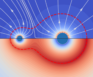
As depicted in figures 3(b,d), in scenarios where $\varphi _{s,1} \neq \varphi _{s,2}$ and $\mathcal {H}$ is relatively small ($\mathcal {H} = 1.1$), it is observed that Droplet 1, which has a lower evaporation potential, exhibits a negative evaporation rate on its side facing the other droplet. This phenomenon essentially manifests as condensation on the surface of one droplet, a result of the high fuel vapour concentration on the surface of its adjacent counterpart. The occurrence of local condensation arises wherever the partial vapour pressure near a liquid surface segment surpasses the saturation pressure. To the best of our knowledge, this effect has not been addressed theoretically in the existing literature on interactive burning droplets, as it is absent in scenarios where both droplets possess identical surface temperatures and consequently the same evaporation potentials.

Our subsequent focus is the distribution of $\varphi$ in certain critical areas for the present problem. These areas of interest include primarily the region along the symmetrical axis, particularly the portion of the axis extending outside the two droplets (indicated by $\theta = 0$), as well as the portion of the axis situated between the two droplets (denoted by $\theta = {\rm \pi}$). The interaction is comparatively weak on the sides of the droplets that are furthest apart from each other. In contrast, the area directly between the droplets, where they face each other, is characterized by the most intense interaction. Based on (4.12), for the portion of the axis extending outside the two droplets ($\theta = 0$), we obtain

(4.15)\begin{align} \varphi (\theta = 0) &\sim |\mathrm{e}^{\xi} - 1 | \times \left[ \left( \frac{1 }{ \mathrm{e}^{\xi - 2\xi_1} - 1 } - \frac{\mathrm{e}^{(\xi_2 - \xi)/2} }{ \mathrm{e}^{\xi_2 - 2\xi_1} - 1 }\,\mathcal{B} (\xi) \right)\mathrm{e}^{- \xi_1}\,\varphi_{s,1} \right.\nonumber\\ &\quad \left.{}+ \left( \frac{1 }{ \mathrm{e}^{2\xi_2 - \xi} - 1 } - \frac{\mathrm{e}^{(- \xi_1 + \xi)/2} }{ \mathrm{e}^{2\xi_2 - \xi_1} - 1 }\,( 1 - \mathcal{B} (\xi) ) \right) \mathrm{e}^{\xi_2 - \xi}\,\varphi_{s,2} \right], \end{align}

while for the portion of the axis located between the two droplets ($\theta = {\rm \pi}$), we have

(4.16)\begin{align} \varphi (\theta = {\rm \pi}) &\sim ( \mathrm{e}^{\xi} + 1 ) \times \left[ \left( \frac{1 }{ \mathrm{e}^{\xi - 2\xi_1} + 1 } - \frac{\mathrm{e}^{(\xi_2 - \xi)/2} }{ \mathrm{e}^{\xi_2 - 2\xi_1} + 1 }\,\mathcal{B} (\xi) \right) \mathrm{e}^{- \xi_1}\,\varphi_{s,1} \right.\nonumber\\ &\quad \left.{}+ \left( \frac{1 }{ \mathrm{e}^{2\xi_2 - \xi} + 1 } - \frac{\mathrm{e}^{(- \xi_1 + \xi)/2} }{ \mathrm{e}^{2\xi_2 - \xi_1} + 1 }\,( 1 - \mathcal{B} (\xi) ) \right) \mathrm{e}^{\xi_2 - \xi}\,\varphi_{s,2} \right]. \end{align}

Figure 4 displays the asymptotic solutions for $\varphi (\theta = 0)$ and $\varphi (\theta = {\rm \pi})$, as detailed in (4.15) and (4.16). These solutions demonstrate good agreement with the numerical solutions, particularly for the portion of the axis extending outside the two droplets ($\theta = 0$), where the asymptotic solution in (4.15) aligns perfectly with the numerical result. As shown in figure 4(a), a smaller inter-droplet distance results in reduced $|\xi |_i$ values, leading to larger gradients of $\varphi$ on the droplet surfaces. This signifies a more intense mass flux on the surface of both droplets in the facing area. According to figure 4(b), when the droplets are closely spaced (i.e. $\mathcal {H} = 1.1$), the variation of $\varphi$ along the portion of the axis located between the two droplets ($\theta = {\rm \pi}$) is generally linear. In this case, the gradients of $\varphi$ on the surfaces of the two droplets exhibit opposite signs, suggesting evaporation on the droplet, with a higher evaporation potential and condensation on the other. As the distance between the droplets increases (e.g. $\mathcal {H} = 3$), this distribution evolves into a concave shape, with a minimum $\varphi$ value between the two droplets. Under these circumstances, the closest points on both droplet surfaces undergo evaporation, leading to the inference that condensation does not occur on either surface.

Figure 4. Distribution of the dimensionless potential function $\varphi / \varphi _{s,i}$ along the symmetrical axis: (a) the portion of the axis extending outside the two droplets (indicated by $\theta = 0$), and (b) the portion of the axis situated between the two droplets (denoted by $\theta = {\rm \pi}$). Here, $r_1 = 100$ ${\rm \mu}$m and $\varphi _{s,2} / \varphi _{s,1} = 1.5$. The scatter data represent numerical results, while the solid lines depict asymptotic solutions provided by (4.15) and (4.16).

Referring to the derivations presented in Appendix A, when the inter-droplet distance becomes substantially large ($\mathcal {H} \to \infty$), the asymptotic solution for $\varphi$ (4.12) can be simplified further. Specifically, for the areas near Droplets 1 and 2, as well as for the region not in close proximity to the surfaces of either droplet, we respectively have

(4.17)\begin{gather} \left.\begin{gathered} \varphi |_{\mathcal{H} \to \infty} ( \xi \to \xi_1 ) \sim \mathrm{e}^{- (\xi - \xi_1)}\, \varphi_{s,1} + ( 1 - \mathrm{e}^{- (\xi - \xi_1)/2} )\, \mathrm{e}^{- \xi_2}\,\varphi_{s,2}, \\ \varphi |_{\mathcal{H} \to \infty} ( \xi \to \xi_2 ) \sim ( 1 - \mathrm{e}^{(\xi - \xi_2)/2} ) \,\mathrm{e}^{\xi_1}\,\varphi_{s,1} + \mathrm{e}^{\xi - \xi_2}\,\varphi_{s,2}, \\ \varphi |_{\mathcal{H} \to \infty} ( \xi \not\to \xi_1, \xi_2 ) \sim ( 1 - \mathrm{e}^{-(\xi_2 - \xi)/2} + \mathrm{e}^{-\xi} ) \,\mathrm{e}^{\xi_1}\, \varphi_{s,1} + ( 1 - \mathrm{e}^{- (\xi - \xi_1)/2} + \mathrm{e}^{\xi}) \,\mathrm{e}^{- \xi_2}\,\varphi_{s,2}, \end{gathered}\right\} \end{gather}

which intuitively demonstrates the interaction between two distant droplets. As stated in (4.17), $\varphi$ is an exclusive function of $\xi$ and remains independent of $\theta$. This implies that when two droplets are significantly separated, the evaporation flux along their surfaces is nearly uniformly distributed. The uniform distribution arises because a large $\mathcal {H}$ value leads to the evaporation of one droplet generating a weak yet consistent concentration of fuel vapour around the other droplet. In such circumstances, the evaporation (or burning) behaviour of each droplet is predominantly governed by its own evaporation potential. The presence of the other droplet exerts a relatively minor effect, as reflected in the expression for $\varphi$ at the limits $\xi \to \xi _1$ and $\xi \to \xi _2$ in (4.17).

4.4. Droplet evaporation/burning rates and interaction coefficients

4.4.1. Droplet evaporation/burning rates

By employing the derived solution for $\varphi$, and leveraging the relationship between local mass flux and $\varphi$ (see (2.12)), the local evaporation rate on the two droplet surfaces can be obtained with

(4.18)\begin{equation} \dot{m}_{ev,i} (\theta) = ({-}1)^{i} \times \left( \frac{\cosh \xi - \cos \theta }{ a }\, \frac{\partial \varphi}{\partial \xi} \right)_{\xi = \xi_i}, \end{equation}

where $(-1)^i$ accounts for the direction of evaporation flux on droplet surfaces. Owing to the axial symmetry of the problem, the evaporation rate $\dot {m}_{ev,i}$ varies as a function of $\theta$, a relationship depicted in figure 5. Note that the horizontal axis in the figure represents the $\theta$ axis in the bispherical coordinate system $(\xi, \theta )$ (refer to figure 1). This axis does not exhibit a uniform variation across the droplet surface. The results shown in figure 5 correspond to a pair of droplets of identical size, where Droplet 2 possesses a slightly larger Spalding number, i.e. $B_{v,2} > B_{v,1}$. It is found that the asymptotic solutions from (4.12) and (4.18) effectively capture the local evaporation rates for both droplets.

Figure 5. Evaporation rate distribution on two equal-sized droplets at varying distances ($r_1 = r_2 = 100$ $\mathrm {\mu }$m; $B_{v,1} = 3$, corresponding to $T_{s,1} \approx 341$ K and $Y_{F,s,1} \approx 0.67$; $B_{v,2} = 4$, corresponding to $T_{s,2} \approx 347$ K and $Y_{F,s,2} \approx 0.74$). The scatter data represent numerical solutions, while the solid lines denote asymptotic solutions provided by (4.12) and (4.18).

Figure 5 reveals distinct $\dot {m}_{ev,i} (\theta )$ distributions due to different droplet temperatures. Droplet 1, at a lower temperature, exhibits a less uniform distribution of evaporation rate compared to the warmer Droplet 2, implying a more significantly impacted evaporation/burning process. When the droplets are distantly spaced (e.g. $\mathcal {H} > 1.5$, not shown in figure 5 for clarity), both possess positive evaporation rates across their surfaces, though the rate diminishes near the facing areas. As the droplets move closer, $\dot {m}_{ev,i} (\theta )$ becomes progressively non-uniform. According to figure 5, as $\mathcal {H}$ falls below a critical threshold, a portion of the Droplet 1 surface facing Droplet 2 experiences condensation instead of evaporation, a phenomenon that intensifies with decreasing $\mathcal {H}$. In contrast, Droplet 2 demonstrates a non-monotonic evaporation rate distribution, featuring an elevated rate on its side facing Droplet 1. Overall, the proximity of the droplets reduces the system's total evaporation rate, attributable primarily to the decreased evaporation rate of the cooler droplet.

By integrating $\dot {m}_{ev,i}$ from (4.18) over the surface of each droplet, their cumulative evaporation rates can be derived as

(4.19)\begin{equation} \dot{Q}_i = \oint_{s,i} \dot{m}_{ev,i} \, \mathrm{d} S = ({-}1)^{i} \times 2 {\rm \pi}a \int_0^{\rm \pi} \left( \mathcal{K} (\xi, \theta)\,\frac{\partial \varphi}{\partial \xi} \right)_{\xi = \xi_i} \mathrm{d} \theta. \end{equation}

Substituting the solution for $\varphi$ (see (4.1)) into (4.19) and integrating yields the cumulative evaporation rates for the two droplets:

(4.20a)$$\begin{gather} \dot{Q}_1 = 8 {\rm \pi}a \sum_{n=0}^\infty \frac{\mathrm{e}^{(2n+1)\xi_1}\,( \varphi_{s,2} - \varphi_{s,1} \,\mathrm{e}^{(2n+1)\xi_2} ) }{ \mathrm{e}^{(2n+1)\xi_1} - \mathrm{e}^{(2n+1)\xi_2} }, \end{gather}$$

(4.20b)$$\begin{gather}\dot{Q}_2 = 8 {\rm \pi}a \sum_{n=0}^\infty \frac{\varphi_{s,1} \,\mathrm{e}^{(2n+1)\xi_1} - \varphi_{s,2} }{ \mathrm{e}^{(2n+1)\xi_1} - \mathrm{e}^{(2n+1)\xi_2} }. \end{gather}$$

According to (4.20), the sign of $\dot {Q}_i$ is determined by the combined effect of the evaporation potentials of both droplet surfaces. Specifically, $\dot {Q}_i$ can be either positive, signifying evaporation, or negative, indicating condensation. This suggests that a droplet may experience either evaporation or condensation collectively, a variability that is absent when the surfaces of both droplets possess identical temperatures. Furthermore, it is crucial to note that the fuel vapour evaporating from each droplet might not fully react with oxygen; instead, it may condense on the surface of the adjacent droplet. Therefore, $\dot {Q}_i$ should be interpreted strictly as the evaporation rate of droplet $i$ and not as a measure of its burning rate.

It is noted that localized condensation on the surface of a droplet can occur when its temperature is lower than that of an adjacent droplet, as depicted in figure 5. However, for the cumulative evaporation rate of a droplet to become negative (i.e. $\dot {Q}_i < 0$), more stringent criteria, as indicated in (4.20), must be satisfied. These criteria necessitate the droplets being in close proximity, with one droplet being comparatively smaller and having a substantially lower temperature than the other.

Utilizing the individual evaporation rates of the two droplets as specified in (4.20), the total evaporation rate of the entire dual-droplet system can be calculated accordingly as

(4.21)\begin{equation} \dot{Q}_{tot} = 8 {\rm \pi}a \sum_{n=0}^\infty \frac{\mathrm{e}^{(2n+1)\xi_1}\,( 1 - \mathrm{e}^{(2n+1)\xi_2} ) \varphi_{s,1} + ( \mathrm{e}^{(2n+1)\xi_1} - 1 ) \varphi_{s,2} }{ \mathrm{e}^{(2n+1)\xi_1} - \mathrm{e}^{(2n+1)\xi_2} } > 0. \end{equation}

Taking into account the signs of $\xi _i$, we can deduce from (4.21) that $\dot {Q}_{tot}$ is invariably positive. This suggests that in scenarios where two adjacent droplets exhibit surface temperature disparities, the system predominantly remains in an evaporation state. This observation persists even when the cooler droplet experiences condensation collectively. Since $\dot {Q}_{tot}$ inherently accounts for the mass transfer between the two droplets, it can also be interpreted as the overall burning rate of the dual-droplet system.

For the special case where the evaporation potentials of the two droplet surfaces are equal ($\varphi _{s,1} = \varphi _{s,2} \equiv \varphi _s$), the individual cumulative evaporation rates of the two droplets, as expressed in (4.20), can be reduced to:

(4.22a)$$\begin{gather} \dot{Q}_1 = 8 {\rm \pi}a \varphi_s \sum_{n=0}^\infty \frac{\mathrm{e}^{(2n+1)\xi_1} ( 1 - \mathrm{e}^{(2n+1)\xi_2} ) }{ \mathrm{e}^{(2n+1)\xi_1} - \mathrm{e}^{(2n+1)\xi_2} }, \end{gather}$$

(4.22b)$$\begin{gather}\dot{Q}_2 = 8 {\rm \pi}a \varphi_s \sum_{n=0}^\infty \frac{\mathrm{e}^{(2n+1)\xi_1} - 1 }{ \mathrm{e}^{(2n+1)\xi_1} - \mathrm{e}^{(2n+1)\xi_2} }. \end{gather}$$

According to (4.22), when $\varphi _{s,1} = \varphi _{s,2}$, both $\dot {Q}_i$ values are greater than $0$, indicating the absence of condensation on each droplet.

Based on (4.20), figure 6 depicts the variation of the cumulative evaporation rates of the two droplets of equal size as their separation distance increases. The Spalding number for Droplet 2 either matches or surpasses that of Droplet 1, leading to the Droplet 2 total evaporation rate being at least as high as that of Droplet 1. In particular, when $B_{v,1} = B_{v,2} = 4$, the evaporation rates of both droplets equalize and converge to a finite value of approximately $\dot {Q}_i \approx 0.8$ kg s$^{-1}$, provided that the droplets are in close proximity ($\mathcal {H} = 1$). As $\mathcal {H}$ increases, their evaporation rates also rise, eventually approaching the limiting value for isolated droplet combustion, estimated at $\dot {Q}_i \approx 1.2$ kg s$^{-1}$.

Figure 6. Theoretical solution for the variation in evaporation rates for two equal-sized droplets at varying distances ($r_1 = r_2 = 100$ $\mathrm {\mu }$m). Here, $B_{v,1} = 4$ is held constant (corresponding to $T_{s,1} \approx 347$ K and $Y_{F,s,1} \approx 0.74$), while $B_{v,2}$ varies among $[4,5,6,7]$ (corresponding to $T_{s,2} \approx [347, 350, 353, 355]$ K and $Y_{F,s,2} \approx [0.74, 0.78, 0.81, 0.84]$).

On the other hand, in cases where $B_{v,2} > B_{v,1}$, the deviation of $\dot {Q}_1$ from $\dot {Q}_2$ increases as the gap between $B_{v,1}$ and $B_{v,2}$ widens. In close proximity, the evaporation rate of Droplet 2 tends towards positive infinity, while that of Droplet 1 approaches negative infinity, representing a singularity of infinite evaporation and condensation rates at their contact point. Despite this, the total evaporation/burning rate $\dot {Q}_{tot}$ of the system remains finite due to the mutual counteraction of these processes. Note that the singularity resulting from the interaction of two droplets with different temperatures is not sustainable in practical scenarios, and serves primarily as a theoretical construct.

4.4.2. Droplet interaction coefficients

In cases where each of the two burning droplets is independently situated in an infinite space, the respective cumulative evaporation rate for each droplet is determined as (Law Reference Law2006; Li et al. Reference Li, Zhang and Law2023b)

(4.23)\begin{equation} \dot{Q}_{iso, i} = 4 {\rm \pi}r_i \times (\rho_g D)_\infty \ln ( 1 + B_{v,i} ) = 4 {\rm \pi}r_i \, \varphi_{s,i}. \end{equation}

Employing the isolated droplet evaporation/burning rate $\dot {Q}_{iso, i}$ given in (4.23) as a reference, the individual interaction coefficients $\eta _i$ for the two droplets, as well as the total interaction coefficient $\eta _{tot}$ for the system, can be determined as

(4.24a,b)\begin{equation} \eta_i \equiv \frac{\dot{Q}_i }{ \dot{Q}_{iso,i} } = \frac{\dot{Q}_i }{4 {\rm \pi}r_i\, \varphi_{s,i}}, \quad \eta_{tot} \equiv \frac{\sum_i \dot{Q}_i }{ \sum_i \dot{Q}_{iso,i} }. \end{equation}

Based on the formulation of $\dot {Q}_i$ as presented in (4.20), the individual interaction coefficients for the two droplets are obtained as

(4.25a)$$\begin{gather} \eta_1 = \frac{2a }{ r_1 } \sum_{n=0}^\infty \frac{\mathrm{e}^{(2n+1)\xi_1}\,( \varphi_{s,2} / \varphi_{s,1} - \mathrm{e}^{(2n+1)\xi_2} ) }{ \mathrm{e}^{(2n+1)\xi_1} - \mathrm{e}^{(2n+1)\xi_2} }, \end{gather}$$

(4.25b)$$\begin{gather}\eta_2 = \frac{2a }{ r_2 } \sum_{n=0}^\infty \frac{(\varphi_{s,1} / \varphi_{s,2})\, \mathrm{e}^{(2n+1)\xi_1} - 1 }{ \mathrm{e}^{(2n+1)\xi_1} - \mathrm{e}^{(2n+1)\xi_2} }. \end{gather}$$

Then, utilizing the expression for $\dot {Q}_{tot}$ in (4.21), the total interaction coefficient for the system can be expressed as

(4.26)\begin{align} \eta_{tot} = \frac{2 a }{ r_1 \varphi_{s,1} + r_2 \varphi_{s,2} } \sum_{n=0}^\infty \frac{\mathrm{e}^{(2n+1)\xi_1}\,( 1 - \mathrm{e}^{(2n+1)\xi_2} ) \varphi_{s,1} + ( \mathrm{e}^{(2n+1)\xi_1} - 1 ) \varphi_{s,2} }{ \mathrm{e}^{(2n+1)\xi_1} - \mathrm{e}^{(2n+1)\xi_2} }> 0. \end{align}

According to (4.25) and (4.26), it is evident that the interaction coefficients $\eta _i$ and $\eta _{tot}$ are affected by the geometric parameters of the system, including the radii of the two droplets $r_i$ and their separation distance $H$. Additionally, these coefficients are influenced by the relative evaporation potential of the droplet surfaces ($\varphi _{s,2} / \varphi _{s,1}$). In particular, in instances where the evaporation potentials of the two droplets are equal, i.e. $\varphi _{s,2} / \varphi _{s,1} = 1$, the interaction coefficients are determined exclusively by the geometric parameters of the system.

Based on (4.25), figure 7 illustrates the variation of $\eta _{i}$ with respect to different droplet radii and distances. It is observed that as $\mathcal {H}$ approaches infinity, $\eta _i$ converges to $1$, signifying minimal interaction. Conversely, at typical droplet distances, $\eta _i$ is less than $1$ and generally decreases with a reduction in $\mathcal {H}$. Notably, when $B_{v,2} = B_{v,1}$, both $\eta _1$ and $\eta _2$ exhibit a gradual decrease as $\mathcal {H}$ reduces, approaching a finite value when $\mathcal {H} \to 1$. In contrast, for $B_{v,2} > B_{v,1}$, a distinct trend is observed: $\eta _1$ decreases rapidly, while $\eta _2$ correspondingly increases sharply as $\mathcal {H}$ descends below a certain threshold. As $\mathcal {H}$ approaches $1$, $\eta _1 \to -\infty$ and $\eta _2 \to +\infty$. This trend is attributed to localized extreme evaporation and condensation rates on the inner sides of the droplets when they are in close proximity, a phenomenon unique to situations where the two droplet surfaces have differing temperatures. A comparison between figures 7(a,b) reveals that as Droplet 1 becomes relatively smaller, its interaction coefficient $\eta _1$ diminishes, indicating a greater suppression of its evaporation rate. Conversely, the interaction coefficient for the larger Droplet 2, $\eta _2$, approaches closer to $1$. Therefore, droplets with higher temperatures and larger radii experience less impact from their neighbouring droplets.

Figure 7. Interaction coefficients for two droplets with varying radii and distances ($r_1 = 100$ $\mathrm {\mu }$m, $B_{v,1} = 4$): (a) $r_2/r_1=1$, (b) $r_2/r_1=2$. The theoretical solution given in (4.25), and the asymptotic solution for $H \to \infty$ given in (4.27) and (4.28), are presented. Here, $\eta = 1$ represents isolated droplet combustion.

4.4.3. Interaction coefficients for two distant droplets

When the two droplets are considerably far apart (i.e. $\mathcal {H} \to \infty$, resulting in $|\xi _i| \to \infty$), based on (4.25) and (4.26), and using the summation formula $\sum _{n=0}^{\infty } \mathrm {e}^{-(2n+1)|\xi |} = 1 / (2 \sinh |\xi |)$, the interaction coefficients for the two droplets can be derived respectively as

(4.27)\begin{equation} \eta_1 |_{\mathcal{H} \to \infty} \sim \frac{a }{ r_1 } \left[ \frac{\varphi_{s,2} / \varphi_{s,1} }{ \sinh (\xi_1 - \xi_2) } - \frac{1 }{ \sinh \xi_1 } \right] \sim 1 - \frac{r_2 }{ H }\,\frac{\varphi_{s,2} }{ \varphi_{s,1} }, \end{equation}

and

(4.28)\begin{equation} \eta_2 |_{\mathcal{H} \to \infty} \sim \frac{a }{ r_2 } \left[ \frac{\varphi_{s,1} / \varphi_{s,2} }{ \sinh (\xi_1 - \xi_2) } + \frac{1 }{ \sinh \xi_2 } \right] \sim 1 - \frac{r_1 }{ H }\,\frac{\varphi_{s,1} }{ \varphi_{s,2} }. \end{equation}

Additionally, the total interaction coefficient can be obtained as

(4.29)\begin{equation} \eta_{tot} |_{\mathcal{H} \to \infty} \sim 1 - \frac{r_1 r_2 }{ H }\, \frac{\varphi_{s,1} + \varphi_{s,2} }{ r_1 \varphi_{s,1} + r_2 \varphi_{s,2} }. \end{equation}

Based on (4.27) and (4.28), it is evident that the interaction coefficient for a droplet reduces as the size and relative evaporation potential of the other droplet increase. As the separation between the two droplets narrows (i.e. $\xi _2 - \xi _1$ decreases), the mutual interference between them intensifies. Notably, when the droplets are substantially separated, their interaction resembles that of point sources. Therefore, the results for $\eta _i$ and $\eta _{tot}$ in the limit of $\mathcal {H} \to \infty$, as determined from (4.27), (4.28) and (4.29), can also be deduced using the point-source method, a technique explored in various studies (Marberry et al. Reference Marberry, Ray and Leung1984; Annamalai & Ryan Reference Annamalai and Ryan1992; Cossali & Tonini Reference Cossali and Tonini2020). However, it is worth mentioning that the existing literature has not explored the impact of differing $\varphi _{s,i}$. Figure 7 compares the asymptotic solutions of $\eta _i$ for two distant droplets with the exact solution from (4.25). It is observed that except in cases involving essentially small $\mathcal {H}$, the asymptotic solution aligns closely with the exact solution. This agreement is particularly apparent for droplets with relatively smaller sizes and Spalding numbers.

Upon comparing the expressions for $\eta _i$ of the two distant droplets, as specified in (4.27) and (4.28), the following relationship is derived:

(4.30)\begin{equation} r_i \varphi_{s,i}^2 (1 - \eta_i) = \frac{r_1 r_2 }{ H } \, \varphi_{s,1} \varphi_{s,2}. \end{equation}

The left-hand side of (4.30) delineates the characteristics of an individual droplet, including its radius, surface evaporation potential and interaction coefficient, while the right-hand side reflects the overall characteristics of the dual-droplet system. This relationship suggests that for a system with distant droplet pairs, the product $r_i \varphi _{s,i}^2 (1 - \eta _i)$ can be considered approximately constant. Consequently, a larger radius $r_i$ and a higher surface evaporation potential $\varphi _{s,i}$ lead to an increased $\eta _i$, simulating a scenario where droplet evaporation and combustion are minimally affected by neighbouring droplets. This finding, in line with our previous discussions, implies that in sparse sprays within a stationary environment, larger and warmer droplets experience less influence from nearby droplets compared to smaller and cooler droplets, which are more susceptible to such influences.

Based on the asymptotic solutions of $\eta _i$ for $\mathcal {H} \to \infty$, as outlined in (4.27) and (4.28), we can deduce that in a multi-droplet burning system with sparsely distributed droplets, their interactions can be linearly superimposed, similar to treating them as point sources. In this context, $\eta _i$ and $\eta _{tot}$ can be expressed as

(4.31a,b) \begin{equation} \eta_i \sim 1 - \sum_{\substack{j = 1 \\ j \neq i}}^{j=N} \frac{r_j }{ H_{ij} }\, \frac{\varphi_{s,j} }{ \varphi_{s,i} }, \quad \eta_{tot} \sim 1 - \frac{1}{ \displaystyle\sum_{i=1}^N ( r_i \varphi_{s,i}) } \times \sum_{i=1}^N \begin{pmatrix}\displaystyle r_i \sum_{\substack{j = 1 \\ j \neq i}}^{j=N} \frac{r_j \varphi_{s,j} }{ H_{ij} } \end{pmatrix}, \end{equation}

where $N$ represents the total number of droplets in the system, $r_j$ is the radius of the $j$th droplet, and $H_{ij}$ is the distance between the $i$th and $j$th droplets. The applicability of (4.31) is $( r_j / H_{ij} ) ( \varphi _{s,j} / \varphi _{s,i} ) \ll 1$ ($i, j = 1, 2, \ldots N$; $j \neq i$). When all droplets in the system maintain the same temperature, and thus the same evaporation potential $\varphi _{s,i}$, the condition simplifies to requiring that the inter-droplet distance be substantially larger than the size of any individual droplet. Conversely, in scenarios where $\varphi _{s,i}$ varies, the condition necessitates that droplets with a higher evaporation potential be positioned farther away from other droplets.

4.4.4. Interaction coefficients for two closely approaching droplets

As the inter-droplet distance reduces, the convergence rate for the infinite series solution of $\eta _i$, detailed in (4.25), becomes slower. In such instances, an integral approach can be employed as a practical approximation for the infinite series. Specifically, for Droplet 1, the value of $\eta _1$ can be approximated using the integral

(4.32a,b)\begin{equation} \eta_1 \approx \frac{2a }{ r_1 } \int_{0}^{\infty} F (n) \,\mathrm{d} n, \quad F (n) \equiv \frac{\mathrm{e}^{(2n+1)\xi_1}\,( \varphi_{s,2} / \varphi_{s,1} - \mathrm{e}^{(2n+1)\xi_2} ) }{ \mathrm{e}^{(2n+1)\xi_1} - \mathrm{e}^{(2n+1)\xi_2}}. \end{equation}

Considering the complexity of the integral in (4.32) under general circumstances, our discussion will focus on the specific case where the two droplets possess equal radii. By employing the defined expression for $F(n)$, the integral in (4.32) can be derived as

(4.33)\begin{equation} \int_{0}^{\infty} F (n) \,\mathrm{d} n = \left( \frac{\varphi_{s,2} }{ \varphi_{s,1} } - 1 \right) \left( \frac{\ln (\mathrm{e}^{2\xi_2} - 1) }{ 4 \xi_2 } - \frac{1 }{ 2 } \right) + \left( \frac{\ln (1 + \mathrm{e}^{\xi_2}) }{2 \xi_2} - \frac{1 }{ 2 } \right). \end{equation}

As two droplets with equal radii approach each other, we can deduce that $a \to r_1 \sqrt {2(\mathcal {H} - 1)}$ and $\mathrm {e}^{\xi _2} \to 1 + \sqrt {2(\mathcal {H} - 1)}$. Utilizing these relationships, the limit of $\eta _1$ as $\mathcal {H} \to 1$ can be determined as

(4.34)\begin{equation} \lim_{\mathcal{H} \to 1} \eta_1 |_{r_1 = r_2} = \ln 2 + \frac{1 }{ 2 } \left( \frac{\varphi_{s,2} }{ \varphi_{s,1} } - 1 \right) \times \lim_{\mathcal{H} \to 1} \ln ( \sqrt{2 (\mathcal{H} - 1)} ). \end{equation}

Similarly, for Droplet 2, the limit of $\eta _2$ as $\mathcal {H} \to 1$ reads

(4.35)\begin{equation} \lim_{\mathcal{H} \to 1} \eta_2|_{r_1 = r_2} = \ln 2 + \frac{1 }{ 2 } \left( \frac{\varphi_{s,1} }{ \varphi_{s,2} } - 1 \right) \times \lim_{\mathcal{H} \to 1} \ln ( \sqrt{2 (\mathcal{H} - 1)} ). \end{equation}

Additionally, the total interaction coefficient for the dual-droplet system can be calculated as

(4.36)\begin{equation} \lim_{\mathcal{H} \to 1} \eta_{tot} |_{r_1 = r_2} = \frac{\varphi_{s,1} \lim_{\mathcal{H} \to 1} \eta_1 |_{r_1 = r_2} + \varphi_{s,2} \lim_{\mathcal{H} \to 1} \eta_2 |_{r_1 = r_2} }{ \varphi_{s,1} + \varphi_{s,2} } = \ln 2. \end{equation}

In cases where $\varphi _{s,1}$ and $\varphi _{s,2}$ differ, (4.34) and (4.35) suggest that $\lim _{\mathcal {H} \to 1} \eta _i = O ( \ln (\mathcal {H} - 1) )$. As the droplets approach each other closely, the interaction coefficient for the droplet with the larger evaporation potential approaches infinity, while for the droplet with the smaller evaporation potential, it tends towards negative infinity. However, in the particular case where $\varphi _{s,1} = \varphi _{s,2}$, $\eta _i (\mathcal {H} \to 1)$ for two equal-sized droplets stabilizes at $\ln 2 \approx 0.693$. This finding aligns with the numerical solutions shown in figure 7(a), and is consistent with previous research (Annamalai & Ryan Reference Annamalai and Ryan1992; Sirignano Reference Sirignano2014). Interestingly, as indicated in (4.36), the total interaction coefficient $\eta _{tot}$ for the system consistently equals $\ln 2$ in close proximity situations, regardless of the relative evaporation potentials. This outcome arises from the counterbalancing of infinite mass transfer at the contact point between the two droplets.

4.5. Flame position and combustion mode transition

The position and morphology of the flame surface are crucial in the analysis of interactive combustion within multi-droplet systems. These aspects play a key role in discerning whether the system exhibits a separated combustion mode or a group combustion mode (Sirignano Reference Sirignano2014). Under the assumption of infinitely fast reactions, the mass fractions of fuel and oxygen on the flame sheet are both reduced to zero (i.e. $Y_F = Y_O = 0$). Therefore, in accordance with the definition of $\beta _{FO}$ in (2.2), it is deduced that $\beta _{FO,f} = \beta _{FO} (\varphi _f) = 0$. Utilizing the solution for $\beta _{FO}$ as presented in (4.11), the value of $\varphi _f$ at the flame surface can be established as

(4.37)\begin{equation} \varphi_f = (\rho_g D)_\infty \ln (1 + \phi Y_{O,\infty}). \end{equation}

Equation (4.37) implies that the flame surface aligns with an isosurface of $\varphi$, a finding consistent with earlier research on multi-droplet systems with identical temperatures (Labowsky Reference Labowsky1980; Imaoka & Sirignano Reference Imaoka and Sirignano2005). As per (4.37), $\varphi _f$ correlates with the oxygen content $Y_{O,\infty }$ in the far field, and remains unaffected by the surface temperature $T_{s,i}$ or the fuel vapour mass fraction $Y_{F,s,i}$ at the droplet surfaces. We introduce a dimensionless quantity $\mathcal {R}_{f,i}$ to quantify the relative distance between the flame surface and individual droplets:

(4.38)\begin{equation} \mathcal{R}_{f,i} \equiv \left( \frac{\varphi_f }{ \varphi_{s,i} } \right)^{{-}1} = \frac{\ln ( 1 + B_{v,i} ) }{ \ln ( 1 + \phi Y_{O,\infty} ) }. \end{equation}

Note that $\mathcal {R}_{f,i}$ represents the relative position of the flame surface within a one-dimensional $\varphi$-based coordinate system, as opposed to its physical location in three-dimensional Cartesian space. The formulation of $\mathcal {R}_{f,i}$ in (4.38) resembles the radius ratio between the flame and droplet surface during the burning of a single, isolated droplet (Sirignano Reference Sirignano2014). According to (4.38), the distance between the flame surface and a droplet within the system increases in response to either a higher evaporation potential of the droplet or a reduced oxygen concentration in the surrounding environment. This observation is believed to apply not only to isolated droplets but also to systems encompassing two or more droplets.

In scenarios where two droplets are significantly distant from each other, each droplet is encircled by a nearly spherical flame, resembling combustion individually in an infinite space, characterizing the system as being in a separated combustion mode. As the droplets approach each other more closely, the shape of their flames starts to change. When the separation becomes sufficiently small, the two distinct flames coalesce into a single flame surface that encompasses both droplets, signifying a transition to group combustion mode. This transition of combustion mode alters the topological properties of the flame surface. Additionally, the operating combustion mode serves as an indicator of the interaction intensity between the burning droplets.

Given the axial symmetry of the problem, the initial point of contact between the two separate flames surrounding the droplets, occurring as $\mathcal {H}$ decreases, is situated along the axis between the surfaces of the two droplets. In cases where the droplets have identical radii and surface potentials, this contact point is precisely at their midpoint $(\xi = 0, \theta = {\rm \pi})$. For more general scenarios, as illustrated in figure 4(b), the criterion for the transition of combustion mode can be established as

(4.39)\begin{equation} \min_{\xi \in [\xi_1, \, \xi_2]} \varphi (\theta = {\rm \pi}) = \varphi_f. \end{equation}

By applying the asymptotic solution for $\varphi (\theta = {\rm \pi})$ from (4.16) into (4.39), the critical droplet distance $\mathcal {H}_{cri}$ that signifies the transition between combustion modes can be determined. Comparing the solution for $\varphi _{s,i}$ (see (4.9)) with the expression for $\varphi _f$ (see (4.37)), it is evident that $\varphi _{s,i}$ is consistently greater $\varphi _f$ across all valid values of $B_{v,i}$ and $\phi Y_{O,\infty }$. This indicates that the minimum value of $\varphi (\theta = {\rm \pi})$ is situated between the surfaces of the two droplets, rather than being directly on either surface. Considering the concave profile of the $\varphi (\theta = {\rm \pi})$ curve, as shown in figure 4, it is demonstrated that during the critical transition of combustion mode, evaporation occurs at the two closest points between the droplets, without any condensation. Accordingly, evaporation is the exclusive process taking place on all surface areas of both droplets. Consequently, the previously discussed phenomenon of partial surface condensation on a droplet, as illustrated in figure 5, is feasible exclusively within group combustion mode.

Based on (4.39), figure 8(a) displays the critical inter-droplet distance $\mathcal {H}_{cri}$ for the transition between combustion modes in a dual-droplet system with varying droplet radii. When $\mathcal {H}$ is greater than $\mathcal {H}_{cri}$, the dual-droplet system displays a separated combustion mode, as depicted in figure 8(b). Conversely, if $\mathcal {H}$ falls below $\mathcal {H}_{cri}$, then the system transitions to a group combustion mode, as shown in figure 8(d).

Figure 8. (a) Critical inter-droplet distance for combustion mode transition ($r_1 = 100$ $\mathrm {\mu }$m). The theoretical solution is calculated based on (4.12) and (4.39), while the asymptotic solution for $r_2 / r_1 \to \infty$ is obtained from (4.40). (b–d) The three typical combustion modes indicated in (a): separated combustion, critical combustion and group combustion modes.

Figure 8(a) shows that for $r_2 / r_1 = 1$, indicating droplets of equal size, the evaporation potentials of both droplets contribute equally to determining $\mathcal {H}_{cri}$. Increasing $B_{v,i}$ results in a greater $\mathcal {H}_{cri}$. Generally, $\mathcal {H}_{cri}$ decreases monotonically as the ratio $r_2 / r_1$ increases. However, in assessing the dimensional counterpart of $\mathcal {H}_{cri}$, represented by $H_{cri} = \mathcal {H}_{cri} (r_1 + r_2)$, it becomes evident that $H_{cri}$ actually increases with an increasing ratio $r_2 / r_1$. It suggests that all else being constant, enlarging the size of either droplet facilitates the interaction between their flames.

In situations with a marked size difference between the two droplets, the contact point of the two distinct flames, during the critical transition of combustion mode, is notably closer to the smaller droplet (see figure 12). In light of this, by applying the asymptotic solution for $\varphi$ from (4.17), the explicit expression for $\mathcal {H}_{cri}$ can be obtained as

(4.40a)$$\begin{gather} \mathcal{H}_{cri} |_{{r_2 }/{ r_1 } \to 0} \sim \left( 1 - \sqrt{1 - \frac{\varphi_f }{ \varphi_{s,2} } } \right)^{{-}1} \frac{\varphi_{s,1} }{ 2 \varphi_{s,2} }, \end{gather}$$

(4.40b)$$\begin{gather}\mathcal{H}_{cri} |_{{r_2 }/{ r_1 } \to \infty} \sim \left( 1 - \sqrt{1 - \frac{\varphi_f }{ \varphi_{s,1} } } \right)^{{-}1} \frac{\varphi_{s,2} }{ 2 \varphi_{s,1}}. \end{gather}$$

According to (4.40), when there is a substantial size difference between the two droplets, resembling a scenario of a droplet adjacent to a large liquid plane, the critical distance $\mathcal {H}_{cri}$ is not determined by the size of the droplets. Instead, it is determined exclusively by $\varphi _f$, which is influenced primarily by $\phi Y_{O,\infty }$, in addition to $\varphi _{s,i}$ of the two droplets. As shown in figure 8(a), when the ratio $r_2 / r_1$ approaches infinity, $\mathcal {H}_{cri}$ approximately converges to the limit specified in (4.40). It is found that this limit is more sensitive to variations in the surface potential of Droplet 2 compared to Droplet 1, indicating that the evaporation potential of the larger droplet exerts a greater influence on the transition between combustion modes.

It should be noted that the results presented in figure 8 are based on the condition where $Y_{O,\infty } = 1$, indicative of an oxygen-rich environment, which brings the flame closer to the droplet surface and results in a smaller $\mathcal {H}_{cri}$. For instance, with $B_{v,1} = B_{v,2} = 1$, $\mathcal {H}_{cri}$ is approximately $4.3$ when $Y_{O,\infty } = 1$, in contrast to approximately $21.8$ in an environment where $Y_{O,\infty } = 0.2$. To provide a clear illustration of the distribution of various physical quantities near the droplet and flame surfaces, subsequent results are obtained based on $Y_{O,\infty } = 1$.

4.6. Solutions for scalar fields and flame temperature distribution

In our above analyses, we have successfully derived both the exact solution, as presented in (4.1), and the asymptotic solution, as per (4.12), for the potential function $\varphi$. Furthermore, as indicated in (4.11), the coupling function $\beta _{FO}$ exhibits a one-to-one correspondence with $\varphi$. This correlation has led to the conclusion that the flame surface aligns with an isosurface of $\varphi$, as outlined in (4.37).

The distribution of fuel vapour and oxygen can be deduced by referencing the definition of $\beta _{FO}$, as presented in (2.2), in conjunction with the flame-sheet assumption. However, to determine the temperature field, it is imperative to find solutions for the additional two coupling functions, $\beta _{TF}$ and $\beta _{TO}$, also defined in (2.2). In cases where the temperatures of the two droplets differ, leading to $\varphi _{s,1} \neq \varphi _{s,2}$, these two coupling functions do not maintain a one-to-one correspondence with $\varphi$ as $\beta _{FO}$ does. Nonetheless, by employing a derivation approach similar to that used for the asymptotic solution of $\varphi$ in Appendix A, we have successfully derived asymptotic solutions for $\beta _{TF}$ and $\beta _{TO}$ as

(4.41)\begin{equation} \beta_k \sim \beta_{k,\infty} - \left[ \frac{\beta_{k,\infty} - \beta_{k,s,1} }{ \mathcal{L} (\varphi_{s,1}) - 1 }\,( 1 - \mathcal{B} (\xi) ) + \frac{\beta_{k,\infty} - \beta_{k,s,2} }{ \mathcal{L} (\varphi_{s,2}) - 1 }\,\mathcal{B} (\xi) \right] ( \mathcal{L} (\varphi) - 1 ), \end{equation}

where $\beta _{k,s,i}$ and $\beta _{k,\infty }$ are specified in the boundary conditions as given in (4.2). Equation (4.41) indicates that $\beta _{TF}$ and $\beta _{TO}$ can be approximated as functions reliant on both $\varphi$ and $\mathcal {B} (\xi )$, which is a bending function ranging from $0$ to $1$ (see (4.13)). Incorporating the boundary conditions for $\beta _{TF}$ and $\beta _{TO}$ from (4.2) into (4.41), the solutions for these two coupling functions can be derived as

(4.42)\begin{align} \beta_{TF} &= \frac{c_{p,g} T_\infty }{ q_c } - \left[ \frac{1 - \mathcal{B} (\xi) }{ \mathcal{L} (\varphi_{s,1}) - 1 } \left( \frac{c_{p,g} (T_\infty - T_{s,1}) }{ q_c } - \frac{Y_{F,s,1} }{ W_F \nu_F } \right) \right. \nonumber\\ &\quad \left.{}+ \frac{\mathcal{B} (\xi) }{ \mathcal{L} (\varphi_{s,2}) - 1 } \left( \frac{c_{p,g} (T_\infty - T_{s,2}) }{ q_c } - \frac{Y_{F,s,2} }{ W_F \nu_F } \right) \right]( \mathcal{L} (\varphi) - 1 ) \end{align}

and

(4.43)\begin{align} \beta_{TO} &= \left( \frac{c_{p,g} T_\infty }{ q_c } + \frac{Y_{O,\infty} }{ W_O \nu_O } \right) - \left[ \frac{1 - \mathcal{B} (\xi) }{ \mathcal{L} (\varphi_{s,1}) - 1 } \left( \frac{c_{p,g} (T_\infty - T_{s,1}) }{ q_c } + \frac{Y_{O,\infty} }{ W_O \nu_O } \right) \right. \nonumber\\ &\quad \left.{}+ \frac{\mathcal{B} (\xi) }{ \mathcal{L} (\varphi_{s,2}) - 1 } \left( \frac{c_{p,g} (T_\infty - T_{s,2}) }{ q_c } + \frac{Y_{O,\infty} }{ W_O \nu_O } \right) \right]( \mathcal{L} (\varphi) - 1 ). \end{align}

Utilizing the solutions for the three coupling functions, namely $\beta _{FO}$, $\beta _{TF}$ and $\beta _{TO}$, as presented respectively in (4.11), (4.42) and (4.43), the scalar fields including $T_g$, $Y_F$ and $Y_O$, for regions both inside and outside the flame surface, can be obtained. These computations are facilitated by integrating the definitions of these coupling functions provided in (2.2). In scenarios of infinitely fast chemical reactions, oxygen does not exist between the droplet and flame surfaces, and fuel vapour is absent beyond the flame surfaces. Consequently, in the region enclosed by the diffusion flame (where $\varphi > \varphi _f$), we have

(4.44a–c)\begin{equation} Y_F = (W_F \nu_F) \times \beta_{FO}, \quad Y_O = 0, \quad T_g = \frac{q_c }{ c_{p,g} } \times \beta_{TO}, \end{equation}

while for the region outside the flame surface (where $\varphi < \varphi _f$), we obtain

(4.45a–c)\begin{equation} Y_F = 0, \quad Y_O ={-} (W_O \nu_O) \times \beta_{FO}, \quad T_g = \frac{q_c }{ c_{p,g} } \times \beta_{TF}. \end{equation}

Upon substituting $\varphi = \varphi _f$ into the solutions for $\beta _{TF}$ and $\beta _{TO}$ given in (4.42) and (4.43), and considering the absence of fuel and oxygen on the flame surface, the temperature distribution along the flame surface can be determined as

(4.46)\begin{align} T_f (\xi)& = T_\infty + \phi Y_{O,\infty} \left[ \frac{1 - \mathcal{B} (\xi) }{ \phi Y_{O,\infty} + Y_{F,s,1} } \left( (T_{s,1} - T_\infty) + \frac{q_c }{ c_{p,g} }\,\frac{Y_{F,s,1} }{ W_F \nu_F } \right) \right. \nonumber\\ &\quad \left.{}+ \frac{\mathcal{B} (\xi) }{ \phi Y_{O,\infty} + Y_{F,s,2} } \left( (T_{s,2} - T_\infty) + \frac{q_c }{ c_{p,g} }\,\frac{Y_{F,s,2} }{ W_F \nu_F } \right)\right]. \end{align}

According to (4.46), contrasting with the results from existing studies based on equal surface temperatures for the droplets (Labowsky Reference Labowsky1980; Umemura et al. Reference Umemura, Ogawa and Oshima1981b; Imaoka & Sirignano Reference Imaoka and Sirignano2005), it is evident that the flame temperature $T_f$ is not uniform when the droplet temperatures are unequal. Given that the chemical energy released during combustion substantially outweighs the internal energy of the evaporated fuel vapour, $T_f$ is influenced primarily by $Y_{F,s,i}$ rather than $T_{s,i}$. In accordance with the Clausius–Clapeyron relation (see (2.14)), which establishes a direct correlation between $Y_{F,s,i}$ and $T_{s,i}$ in thermodynamic equilibrium, elevating the surface temperature of a droplet notably increases its adjacent flame temperature, whereas lowering the droplet's temperature reduces the flame temperature on that side.

Based on (4.46), figure 9 presents the theoretical flame temperature distribution. For the case with $B_{v,1} = 1$ and $B_{v,2} = 2$, the respective surface temperatures of the two droplets are approximately $315\ {\rm K}$ and $333\ {\rm K}$. Despite the modest difference of $18\ {\rm K}$ in droplet surface temperatures, a substantial temperature variation becomes apparent on the flame surface, with the maximum discrepancy exceeding $200\ {\rm K}$. This substantial variation suggests that differences in surface fuel vapour concentrations, stemming from the distinct droplet surface temperatures, are the primary factors contributing to the observed uneven temperature distribution on the flame surface.

Figure 9. Theoretical distribution of flame temperature outside the two droplets at varying droplet distances and sizes ($r_1 = 100$ $\mathrm {\mu }$m; $B_{v,1} = 1$, corresponding to $T_{s,1} \approx 315\ {\rm K}$ and $Y_{F,s,1} \approx 0.35$; $B_{v,2} = 2$, corresponding to $T_{s,2} \approx 333\ {\rm K}$ and $Y_{F,s,2} \approx 0.57$). The theoretical solution is calculated using (4.12), (4.37) and (4.46).

In scenarios where $B_{v,2} > B_{v,1}$, as depicted in figure 9, the lowest temperature on the flame surface resides at the outermost side of Droplet 1, denoted as $T_{f,out,1}$, while the highest temperature is found at the outermost side of Droplet 2, identified as $T_{f,out,2}$. When $\mathcal {H}$ is smaller than $\mathcal {H}_{cri}$, a unified flame surface encompasses both droplets, resulting in a gradual transition of flame temperature $T_f$ from $T_{f,out,1}$ to $T_{f,out,2}$ along the flame surface. In contrast, when $\mathcal {H}$ surpasses $\mathcal {H}_{cri}$, the flame surface surrounding the droplets separates, leading to two distinct temperature discontinuities. These discontinuities are located at the nearest points of the two separate flames, with the temperatures at these points identified as $T_{f,in,1}$ and $T_{f,in,2}$, respectively. The $T_{f,in,i}$ value for each droplet rapidly approaches its corresponding $T_{f,out,i}$ value for increasing $\mathcal {H}$, indicating a more uniform temperature distribution across each flame surface. According to figure 9, as $\mathcal {H}$ approaches infinity, both $T_{f,in,i}$ and $T_{f,out,i}$ converge to $T_{f,iso,i}$, which represents the flame temperature of Droplet $i$ when it burns in isolation.

Figure 9 provides additional insight into the influence of the relative sizes of the two droplets on the range of flame temperatures. Specifically, within the group combustion mode, an increase in the size of Droplet 2 results in a higher maximum temperature $T_{f,out,2}$ on the flame surface. This increase in the maximum temperature also simultaneously raises the minimum temperature of the flame surface, $T_{f,out,1}$. However, when the system transitions into the separated combustion mode, the sensitivity of the variation in flame temperatures to the relative sizes of the droplets diminishes.

Figure 10 displays the contours of various physical quantities during the QS combustion of two interacting droplets, identical in both temperature and radius. A comparison with numerical solutions reveals that the asymptotic solutions, derived from (4.11), (4.12), (4.42) and (4.43), effectively capture variations in the flow, composition and temperature fields at different inter-droplet distances. It is seen that with droplets at equal temperatures, the flame temperature distribution remains uniform. When the droplets are in close proximity, as shown in figure 10(a) with $\mathcal {H} = 1.5$, they are enveloped by an ellipsoidal-shaped flame. As the inter-droplet distance increases, as depicted in figure 10(b) with $\mathcal {H} = 3$, the ellipsoidal flame stretches, and the Stefan flow intensifies around both droplets, particularly on their adjacent sides. Further increase of $\mathcal {H}$, as illustrated in figure 10(c) with $\mathcal {H} = 5$, leads to the division of the enveloping flame into two distinct flames, each surrounding one droplet. These two separate flames initially exhibit an inward-pointing egg shape around each droplet. As $\mathcal {H} \to \infty$, the two flames gradually transition into spherical shapes, with the evaporation and combustion dynamics of each droplet mirroring that of an isolated droplet.

Figure 10. Distributions of various physical quantities during the combustion of two droplets of equal size and temperature at varying distances ($r_1 = r_2 = 100$ $\mathrm {\mu }$m; $B_{v,1} = B_{v,2} = 1$, corresponding to $T_{s,i} \approx 315\ {\rm K}$ and $Y_{F,s,i} \approx 0.35$). Asymptotic solutions, calculated primarily using (4.11), (4.12), (4.42) and (4.43), are compared with numerical solutions.

In contrast to the special case of equal-temperature droplets shown in figure 10, figure 11 presents a more general scenario involving droplets with disparate temperatures, as indicated by their differing Spalding numbers. It is evident that our theoretical solutions maintain a close alignment with the numerical results. In figure 11, the Spalding number for Droplet 2, $B_{v,2}$, is increased from $1$ to $2$, in contrast to the case shown in figure 10. As a result, Droplet 2 exhibits a higher temperature and fuel vapour concentration on its surface, which is visible in figures 11(a iii), 11(b iii) and 11(c iii). This leads to a faster evaporation rate for Droplet 2, causing its adjacent flame surface to be located further from the droplet surface. A comparison between figures 10(c) and 11(c) reveals that a higher Spalding number for either of the droplets increases the probability of group combustion and reinforces the interaction between the droplets. In contrast to the uniform flame temperature distribution observed in figure 10, scenarios involving differing droplet temperatures, as shown in figure 11, display a non-uniform temperature distribution across the flame surface. This non-uniformity is characterized by notably lower flame temperatures near Droplet 1 in comparison to the flame temperatures observed on the side of Droplet 2.

Figure 11. Distributions of various physical quantities during the combustion of two droplets of equal size but unequal temperatures at varying distances ($r_1 = r_2 = 100$ $\mathrm {\mu }$m; $B_{v,1} = 1$, corresponding to $T_{s,1} \approx 315\ {\rm K}$ and $Y_{F,s,1} \approx 0.35$; $B_{v,2} = 2$, corresponding to $T_{s,2} \approx 333\ {\rm K}$ and $Y_{F,s,2} \approx 0.57$). Asymptotic solutions, calculated primarily using (4.11), (4.12), (4.42) and (4.43), are compared with numerical solutions.

While this study focuses primarily on the QS combustion of two interacting droplets with differing temperatures by assuming infinitely fast reactions, the insights gained are invaluable for understanding important phenomena associated with finite-rate reactions, such as flame spreading, as well as local flame extinction and ignition, in multi-droplet systems (Brzustowski et al. Reference Brzustowski, Sobiesiak and Wojcicki1981; Mikami et al. Reference Mikami, Oyagi, Kojima, Wakashima, Kikuchi and Yoda2006, Reference Mikami, Matsumoto, Chikami, Kikuchi and Dietrich2023; Yoshida et al. Reference Yoshida, Iwai, Nagata, Seo, Mikami, Moriue, Sakashita, Kikuchi, Suzuki and Nokura2019). In scenarios involving finite-rate reactions, the high sensitivity of combustion reactions to temperature variations is crucial. A reduction in temperature at any segment of the flame surface can potentially cause local flame extinction (Farouk & Dryer Reference Farouk and Dryer2023). In the context of the present dual-droplet system, such local extinction is likely to occur near the cooler droplet, resulting in the leakage of unburned fuel vapour. Conversely, raising the temperature of either one or both droplets in the pair may lead to local ignition and flame spreading.

Indeed, in real-world scenarios, droplet temperatures are influenced by their surroundings, including heat transfer through thermal conduction and radiation from the flames. In this context, when a burning droplet approaches an unignited, cold droplet, two primary outcomes are possible. First, the cold droplet can be heated up substantially, eventually leading to its ignition, and potentially resulting in group combustion involving both droplets. Alternatively, the burning droplet could cool down considerably, with a significant reduction in its flame temperature, which may cause flame extinction. For simplicity, this paper focuses exclusively on scenarios with fixed droplet temperatures, enabling valuable discussions regarding the one-way influence of droplet temperatures on flame temperature distributions in dual-droplet systems. To comprehensively address the intricate aspects of transient ignition, extinction and flame spreading in such systems, further research and advanced modelling efforts are essential.

Note that figures 10 and 11 illustrate cases of droplets with equal radii; figure 12 broadens the scope to include a more general situation with droplets that have unequal radii. Specifically, Droplet 2 has a radius double that of Droplet 1. Figures 12(a–d) display the situation where $B_{v,2} / B_{v,1} = 0.5$, while figures 12(e–h) depict the scenario when the ratio is $2$. These figures reveal that a larger droplet radius enhances inter-droplet interaction, enlarges the flame, and delays flame separation as $\mathcal {H}$ increases. In figures 12(a–d), despite Droplet 2 being larger, its lower evaporation potential results in a flame size comparable to that of Droplet 1. Conversely, figures 12(e–h) show Droplet 2 as having both a larger radius and a greater evaporation potential, leading to a notably larger flame surface. In this instance, the evaporation and combustion process of the dual-droplet system is dominated primarily by the characteristics of Droplet 2. The flame shape and size around Droplet 2 remain relatively unchanged, irrespective of the inter-droplet distance or the combustion mode. Droplet 2 exhibits a comparatively uniform evaporation rate, characterized by spherically symmetric streamlines in the contours. In contrast, Droplet 1 shows a more variable evaporation rate with disturbed streamlines, particularly at small droplet distances (see figure 12e). Notably, regions exhibiting higher flame temperatures are consistently located closer to the droplet with a higher evaporation potential. This observation holds regardless of the relative sizes of the two droplets, in accordance with the theoretical solution presented in (4.46).

Figure 12. Theoretical solutions for the flow and temperature fields during the combustion of two droplets with dissimilar radii and temperatures at various inter-droplet distances ($r_1 = 100$ $\mathrm {\mu }$m, $r_2 = 200$ $\mathrm {\mu }$m). The theoretical solutions are calculated using (4.11), (4.12), (4.42) and (4.43).

It should be noted that more intricate evaporation/condensation and combustion phenomena are anticipated with multi-component droplets or those exhibiting non-uniform temperature distributions (Sirignano & Wu Reference Sirignano and Wu2008; Cira, Benusiglio & Prakash Reference Cira, Benusiglio and Prakash2015; Tonini & Cossali Reference Tonini and Cossali2016; Diddens et al. Reference Diddens, Kuerten, Van der Geld and Wijshoff2017; Wang et al. Reference Wang, Orejon, Takata and Sefiane2022). However, these complexities are outside the scope of the current study.