1. Introduction
Neutral hydrogen (HI) provides the raw material for the formation of stars and so the abundance of this at various redshifts should closely trace the star-forming activity over the history of the Universe. Specifically, the star formation rate density, ψ *, exhibits a steep climb from z = 0 before peaking at z ∼ 2.5, followed by a steep decline at higher redshifts (Hopkins & Beacom Reference Hopkins and Beacom2006; Burgarella et al. Reference Burgarella2013; Sobral et al. Reference Sobral, Smail, Best, Geach, Matsuda, Stott, Cirasuolo and Kurk2013; Lagos et al. Reference Lagos, Baugh, Zwaan, Lacey, Gonzalez-Perez, Power, Swinbank and van Kampen2014; Madau & Dickinson Reference Madau and Dickinson2014; Zwart et al. Reference Zwart, Jarvis, Deane, Bonfield, Knowles, Madhanpall, Rahmani and Smith2014). However, the mass density of the neutral gas exhibits very little redshift evolution: Over 0 ≲ z ≲ 0.5, where HI 21-cm can be detected in emission (e.g. Fernández et al. Reference Fernández2016), the mass density is ΩHI ≈ 0.5 × 10⁻³ (Zwaan et al. Reference Zwaan, van der Hulst, Briggs, Verheijen and Ryan-Weber2005; Lah et al. Reference Lah2007; Braun Reference Braun2012; Delhaize et al. Reference Delhaize, Meyer, Staveley-Smith and Boyle2013; Rhee et al. Reference Rhee, Zwaan, Briggs, Chengalur, Lah, Oosterloo and van der Hulst2013; Hoppmann et al. Reference Hoppmann, Staveley-Smith, Freudling, Zwaan, Minchin and Calabretta2015). At higher redshift, where the HI column density is obtained from either space (z ≲ 1.7) or ground (z ≳ 1.7) based observations of damped Lyman-α systems (DLAs, where N HI ≥ 2 × 1020 cm−2),Footnote a the mass density rises to ΩHI ≈ 1 × 10⁻³, remaining constant up to at least z ∼ 5 (Rao & Turnshek Reference Rao and Turnshek2000; Prochaska & Herbert-Fort Reference Prochaska and Herbert-Fort2004; Rao, Turnshek & Nestor Reference Rao, Turnshek and Nestor2006; Curran Reference Curran2010; Prochaska & Wolfe Reference Prochaska and Wolfe2009; Noterdaeme et al. Reference Noterdaeme2012; Crighton et al. Reference Crighton2015; Neeleman et al. Reference Neeleman, Prochaska, Ribaudo, Lehner, Howk, Rafelski and Kanekar2016). Thus, there is a clear disparity between the star formation density and the neutral gas available to fuel it.
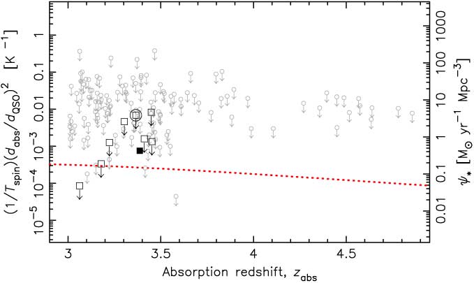
The Lyman-α (λ = 1215.67 Å) transition traces all of the neutral gas, specifically both the cold (CNM, where T ∼ 150 K and n ∼ 10 cm−3) and warm neutral media (WNM, where T ∼ 10 000 K and n ∼ 0.2 cm−3, Field, Goldsmith & Habing Reference Field, Goldsmith and Habing1969; Wolfire et al. Reference Wolfire, Hollenbach, McKee, Tielens and Bakes1995). Given that only the gas clouds which are cool enough to collapse under their own gravity are expected to initiate star formation, we may only expect the cool component, the CNM, to follow the star formation history. Radio-band 21-cm absorption traces this component of the hydrogen, and the comparison of this with the total column density provides a temperature measure of the gas. Using this method, Curran (Reference Condon, Cotton, Greisen, Yin, Perley, Taylor and Broderick2017a) showed that the spin temperature and the star formation density may be inversely related (Figure 1). As seen from the figure, however, while 1/T spin (degenerate with the ratio of the absorber and emitter extents, d abs/d QSO) does follow a similar increase as ψ * up to the z ∼ 2.5 peak, what happens beyond this is as yet unknown. In this paper, we explore the feasibility of obtaining the required data with current state-of-the-art radio telescopes, in addition to exploring the prospects with the Square Kilometre Array (SKA).

Figure 1. The cosmological mass density of neutral hydrogen (solid trace, Crighton et al. Reference Crighton, Gil de Paz, Knapen and Lee2017) and the star formation density (dotted trace, Hopkins & Beacom Reference Hopkins and Beacom2006) versus redshift. The error bars show the binned (n = 50 per bin) ±1σ values of (1/T spin)(d abs/d QSO)2, normalised on the ordinate by 500 M⊙ yr−1 Mpc−3 K (Curran, Reference Curran2017b).
2. The sample
From Figure 1 it is clear that higher redshift (z abs ≳ 3) data are required in order to determine whether the spin temperature, degenerate with the ratio of the absorber/emitter extent, is anti-correlated with the star formation density, or whether it just (coincidentally) increases by the same approximate factor out to the peak ψ *. Since we wish to find the typical sensitivity limits attainable by current and future facilities, we require a large readily available sample of DLAs. Such a sample is provided by the spectra of quasi-stellar objects (QSOs) in the Sloan Digital Sky Survey (SDSS), which provides the largest catalogue of DLAs (Prochaska & Herbert-Fort Reference Prochaska and Herbert-Fort2004; Prochaska et al. Reference Prochaska, Herbert-Fort and Wolfe2005; Noterdaeme et al. Reference Noterdaeme, Petitjean, Ledoux and Srianand2009), with the SDSS-III DR9 DLA (Noterdaeme et al. Reference Noterdaeme2012) being the most recently published catalogue of reliable absorbers.Footnote b This contains 12 081 DLAs and sub-DLAs (all with N HI ≥ 1 × 1020 cm−2), over redshifts of 1.951 ≤ z abs ≤ 5.343.
We match each QSO to the nearest radio source (within 10 arcsec) in each of the NRAO VLA Sky Survey (NVSS, Condon et al. Reference Condon, Cotton, Greisen, Yin, Perley, Taylor and Broderick1998), the Very Large Array’s Faint Images of the Radio Sky at Twenty-Centimeters (FIRST, White et al. Reference White, Becker, Helfand and Gregg1997), and the Sydney University Molonglo Sky Survey (SUMSS, Mauch et al. Reference Mauch, Murphy, Buttery, Curran, Hunstead, Piestrzynski, Robertson and Sadler2003). This yields 336 radio-loud sight-lines, containing a total of 414 absorbers (Figure 2). For each of the large radio interferometers, the Murchison Widefield Array (MWA), the Low-Frequency Array (LOFAR), the Giant Metrewave Radio Telescope (GMRT), the Very Large Array (VLA), as well as the forthcoming SKA, we determine which of the DLAs occulting a radio-loud source would have the 21-cm transition redshifted into an available band. From an estimate of the flux density, we then determine the best expected sensitivity of the instrument and whether this is sufficient to detect the putative high redshift downturn in 1/T spin (Figure 1). Note that we do not include large single dish instruments (e.g. the Green Bank Telescope, GBT) due to the restrictions in mitigating the radio frequency interference (RFI) at these frequencies (e.g. Curran et al. Reference Curran, Allison, Whiting, Sadler, Combes, Pracy, Bignell and Athreya2016a).
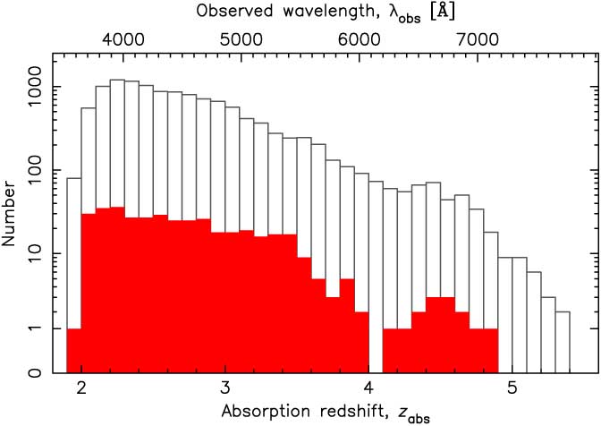
Figure 2. The redshift distribution of the DR9 DLAs (unfilled histogram) overlaid with those occulting a known radio source (filled histogram).
3. Analysis
3.1. Attainable limits
From the radiometer equation (e.g. Rohlfs & Wilson Reference Rohlfs and Wilson2000), the r.m.s. noise level obtained after an integration time of t int is given by
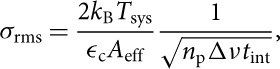 $${\sigma _{{\rm{rms}}}} = {{2{k_{\rm{B}}}{T_{{\rm{sys}}}}} \over {{\epsilon_{\rm{c}}}{A_{{\rm{eff}}}}}}{1 \over {\sqrt{{n_{\rm{p}}}\Delta \nu {t_{{\rm{int}}}}} }},$$
where k B is the Boltzmann constant, T sys the system temperature, ɛc the correlator efficiency, A eff the effective collecting area of the telescope, n p the number of polarisations, and Δv is the channel bandwidth. This is related to the velocity resolution, Δv, via Δv = (Δv/c)v obs, where c is the speed of light and v obs is the observed frequency.
The observed optical depth, τ obs, of the absorption is given by the ratio of the line depth, ΔS, to the observed background flux, S, and is related to the intrinsic optical depth, τ, via
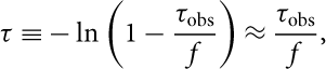 $$\tau \equiv - \ln\left( {1 - {{{\tau _{{\rm{obs}}}}} \over f}} \right) \approx {{{\tau _{{\rm{obs}}}}} \over f},$$
in the optically thin regime (ΔS/S ≲ 0.3), where the covering factor, f, is the fraction of S intercepted by the absorber. In the case of a 3σ upper limit, the optical depth is thus given by τ obs ≲ 3σ rms/S.
Using the flux density (see 3.2), we can therefore estimate the upper limits to the observed velocity-integrated optical depth. Inserting ∫τ obs dv ≤ (3σ rms/S) Δv per Δv channel (see Curran Reference Curran2012) into N Hi = 1.823 × 10¹⁸ T spin ∫τ dv (Wolfe & Burbidge Reference Wolfe and Burbidge1975) gives
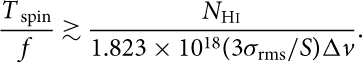 $$\frac{T_\textrm{ spin}}{f} \gtrsim \frac{N_\textrm{H\textsc{i}}}{1.823\times10^{18} (3\sigma_\textrm{rms}/S)\Delta v}.$$
Providing that the Lyman-α and 21-cm absorption arise along the same sight-line, Equation (3) yields the limit to the spin temperature of the gas attainable by each instrument. T spin is a measure of the excitation of the gas by 21-cm absorption (Purcell & Field Reference Purcell and Field1956), excitation above ground state by Lyman-α absorption (Field Reference Field1959), and collisional excitation (Bahcall & Ekers Reference Bahcall and Ekers1969). This provides a thermometer—allowing a measure of the fraction of the CNM—the cool gas in which star formation occurs. The spin temperature is, however, degenerate with the covering factor (Equation (3)), whose value requires knowledge of the relative extents of the absorber–frame 1 420 MHz absorption and emission cross-sections (d abs/d QSO). This can, however, be expressed as
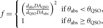 $$f = \left\{{\matrix{{{{\left( {{{{d_{{\rm{abs}}}}D{A_{{\rm{QSO}}}}} \over {{d_{{\rm{QSO}}}}D{A_{{\rm{abs}}}}}}} \right)}^2}} \hfill& {\;{\rm{if}}\;{\theta _{{\rm{abs}}}} \lt {\theta _{{\rm{QSO}}}},} \hfill\cr \\ 1 \hfill& {{\rm{if}}\;{\theta _{{\rm{abs}}}} \ge{\theta _{{\rm{QSO}}}},} \hfill\cr} }\right.$$
where DA abs and DA QSO are the angular diameter distances and θ abs and θ QSO the angular extents of the absorbers and emitter, respectively (Curran Reference Curran2012).
The angular diameter distance is obtained from line-of-sight co-moving distance, DC, (e.g. Peacock Reference Peacock1999),
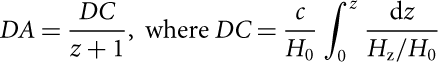 $$DA = {{DC} \over {z + 1}} ,\ {\rm {where}}\;DC = {c \over {{H_0}}}\int_0^z {{{\rm {d}}z} \over {{H_{\rm {z}}}/{H_0}}}$$
in which c is the speed of light, H 0 the Hubble constant, H z the Hubble parameter at redshift z, and
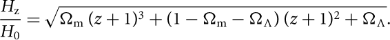 $${{{H_{\rm {z}}}} \over {{H_0}}} = \sqrt {{\Omega _{\rm {m}}}{\kern 1pt} {{(z + 1)}^3} + (1 - {\Omega _{\rm {m}}} - {\Omega _\Lambda }){\kern 1pt} {{(z + 1)}^2} + {\Omega _\Lambda }}.$$
For a standard Λ cosmology, with H 0 = 71 km s −1 Mpc−1, Ωm = 0.27 and, ΩΛ = 0.73, this gives a range of possible values of DA abs/DA QSO at, z abs ≲ 1.6 whereas above this redshift the ratio of angular diameter distances is always close to unity, i.e. DA abs/DA QSO ∼ 1, ∀z abs ≳ 1.6. If left uncorrected, this will introduce a bias to the covering factors between low and high redshift DLAs (Curran & Webb Reference Curran and Webb2006). Correcting for this, by inserting Equation (4) into Equation (3), gives
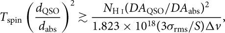 $$T_\textrm{spin}\left(\frac{d_\textrm{QSO}}{d_\textrm{abs}}\right)^2 \gtrsim\frac{N_\textrm{H \textsc{i}}(DA_\textrm{QSO}/DA_\textrm{abs})^2}{1.823\times10^{18} (3\sigma_\textrm{rms}/S)\Delta v},$$
for f < 1, which is expected for the high redshift absorbers (Curran Reference Curran2017a).
Binning the current 21-cm absorption data, the spin temperature degenerate with the ratio of the emitter–absorber extent, (1/T spin)(d abs/d QSO)2, traces the star formation density up to the redshift limit of the data (Figure 1) and reproduces the observed CNM fractions in DLAs for a mean 〈d QSO/d qbs〉 ∼ 4 (Curran Reference Curran2017b). With Equation (5), we can estimate the attainable limit for each radio-illuminated DLA in the SDSS DR9 and whether its addition to the current data could help determine if (1/T spin)(d abs/d QSO)2 follows the ψ * downturn at z abs ≳ 3.
3.2. Radio fluxes
For each of the 336 radio-loud sight-lines (Section 2), we obtain the radio photometry from NASA/IPAC Extragalactic Database (NED) and estimate the flux density from the background source at the redshifted 21-cm frequency of each DLA, via a fit in logarithm space:
– for at least four radio-band photometry points, a second-order polynomial, according to the prescription of Curran et al. (Reference Curran, Whiting, Sadler and Bignell2013),
– for two or three radio-band photometry points, a first-order polynomial (a power law),
– for a single radio-band photometry point, we assume a spectral index. Values of α ≈ −1 are typical of z ≳ 3 radio sources (e.g. De Breuck et al. Reference De Breuck, van Breugel, Stanford, Röttgering, Miley and Stern2002; Curran et al. Reference Curran, Whiting, Sadler and Bignell2013), although there may be a redshift dependence (Athreya & Kapahi Reference Athreya and Kapahi1998).
There are 14 sources which are fit by the second-order polynomial and 58 fit by a power law, leaving 264 requiring an estimate of the spectral index. In Figure 3 we show how the spectral indices of the 58 power law fits vary with redshift. From this, it is clear that, since the measured flux is generally at a higher frequency than the redshifted 21-cm absorption (Figure 4), assuming too steep a spectral index could significantly overestimate the flux density. Rather than assuming α = −1, we therefore use a redshift-dependent spectral index, where α = −0.087 z QSO – 0.175 (Figure 3). The resulting flux density distribution is shown in Figure 5.
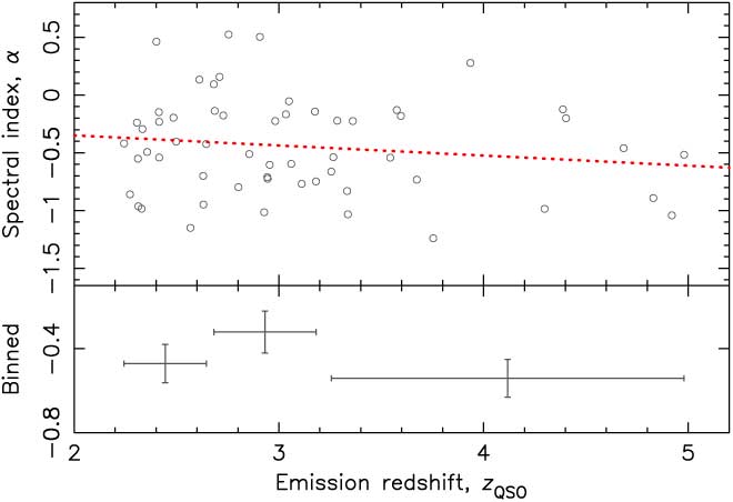
Figure 3. The radio-band spectral index versus redshift for the 58 SED (spectral energy distribution) fit by a power law, where the dotted line shows the least-squares fit. The bottom panel shows the binned values in equally sized bins, where the horizontal error bars show the range of points in the bin and the vertical error bars the error in the mean value.
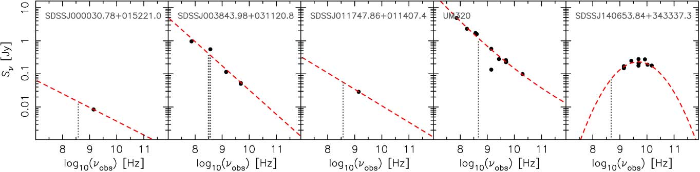
Figure 4. Examples of SED fits to the radio photometry of the background sources. The vertical dotted lines show the frequency of the 21-cm transition at the absorber redshift (the second source has four intervening absorbers).
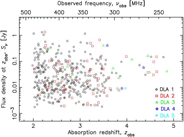
Figure 5. The flux density estimated at the absorption redshift. The colour/shape of the symbol indicates which absorber, since some sight-lines have multiple DLAs—48 sight-lines with a second DLA, ten with a third, two with a fourth and one with a fifth.
3.3. Prospects with current instruments
3.3.1. Murchison Widefield Array
The MWA (Tingay et al. Reference Tingay2013) has a coverage of 80–300 MHz, which spans HI 21-cm at redshifts of z abs > 3.735. For declinations of δ < 33°, this range gives 15 DLAs illuminated by a radio source observable by the MWA. The spectrometer is limited to a channel spacing of ≥ 10 kHz, which corresponds to a spectral resolution of Δv ≥ 10 km s−1 at v obs ≤ 300 MHz.Footnote c At v obs = 200 MHz and T sys = 195 K, using all 128 tiles (A eff = 2 534 m2) gives a theoretical r.m.s. noise level of σ rms = 11 mJy per 10 kHz channel after t int = 10 h per sight-line (Equation (1)).Footnote d From a search for Hi 21-cm absorption within the hosts of high redshift radio sources,Footnote e a multiplicative (fudge) factor of ≈2 is found, i.e. we should expect an r.m.s. noise level of σ rms ≈ 22 mJy per 10 kHz channel. Combining this with the estimated flux densities, we obtain limits of (1/T spin)(d abs/d QSO)2 ≳ 0.01 K−1, which are insufficient to confirm the putative downturn in (1/T spin)(d abs/d QSO)2 at z ≳ 3 (Figure 6).
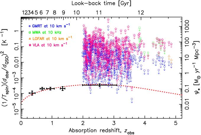
Figure 6. As Figure 1, but showing the 3σ limits in (1/T spin)(d abs/d QSO)2 reached after 10 h of integration at a spectral resolution of 10 km s−1 per channel for the current instruments.
3.3.2. Low-Frequency Array
LOFAR (van Haarlem et al. Reference van Haarlem2013) has a frequency range of 10–250 MHz, which covers the 21-cm transition for only two of the DR9 DLAs, with the δ > −7° declination limit imposing no additional cut. From the point source sensitivity (Figure 7), t int = 10 h gives an r.m.s. noise level of σ rms = 11 − 13 mJy per 10 km s−1 channel, cf. the theoretical 1.5 mJy using all stations (24 core, 14 remote, and 13 international). A fudge factor of ≲ 10 in the noise level is expected,Footnote f giving the values in Figure 7, although spectral line observations suggest that this should be 3–5 (e.g. Oonk et al. Reference Oonk2014). Applying a factor of 4 gives σ rms = 5.4 – 6.5 mJy per 10 km s−1 channel and limits of (1/T spin)(d abs/d QSO)2 ∼ 0.01 K−1, which are, again, insufficient to detect the downturn (Figure 6).

Figure 7. Polynomial fits to the system equivalent flux density of LOFAR (van Haarlem et al. Reference van Haarlem2013).
3.3.3. (Upgraded) Giant Metrewave Radio Telescope
For the GMRT (Ananthakrishnan Reference Ananthakrishnan1995), there are two bands available which can detect 21-cm over the redshift range of the DR9 DLAs—the 230–250 and 250–500 MHz bands, the latter of which is currently being commissioned as part of the upgraded GMRT (uGMRT). Combining these gives 414 sight-lines towards a radio-loud source for which 21-cm is redshifted to 230–500 MHz and is at a declination observable with the GMRT (δ ≳ −40°). In order to calculate the telescope sensitivity, we estimate the system temperature by interpolating the values quoted for the 151, 235, and 325 MHz bands,Footnote g giving T sys = 0.0175v obs2 – 11.2v obs + 1915, where v obs is in MHz, resulting in T sys = 106 – 215 K for the sample. For a t int = 10 h integration using all 30 antennas (A eff = 26 508 m2) and a fudge factor of 5 in the time estimate,Footnote h we reach σ rms = 1.3 − 16 mJy per 10 km s−1 channel.
The radiometer equation Equation (1) gives the theoretical noise level, which can be significantly lower than the actual value obtained in the production of an image (e.g. 3.3.2). The fudge factor is intended to correct for this and, in order to check the validity of the value used, we show actual measured sensitivities (Table 1) in comparison to our predicted limits (Figure 8). From this we see that the predicted values are close to those observed and that the fudge factor may even overcompensate the correction somewhat. Using these conservative estimates, however, we see that sufficiently sensitive limits, (1/T spin)(d abs/d QSO)2 ∼ 10−4 K−1, are attainable, although only at redshifts of z abs ≲ 3.5 (Figure 6).
Table 1. The z abs > 3 DLAs searched for HI 21-cm absorption
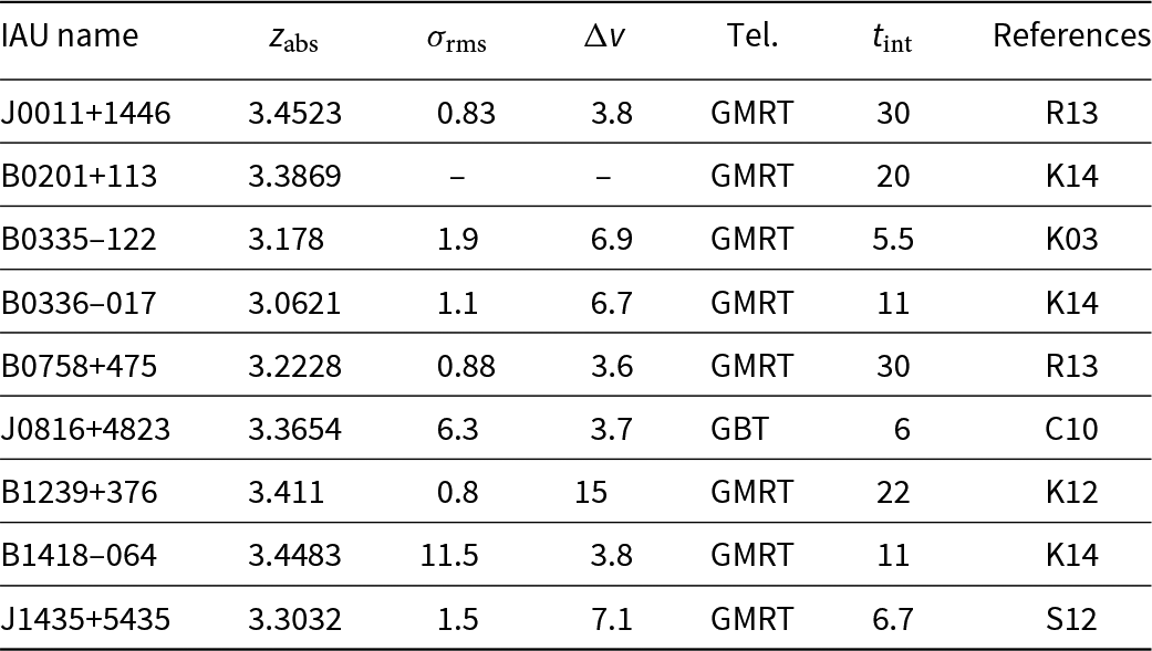
σ rms [mJy] is the r.m.s. noise level per Δv [km s−1] channel after t int [hours] obtained with the listed telescope. The absorber towards B0201+113 is detected in 21-cm absorption with ∫ τ obs dv = 0.71 km s−1
References: K03—Kanekar & Chengalur (Reference Kanekar and Chengalur2003), C10—Curran et al. (Reference Curran, Tzanavaris, Darling, Whiting, Webb, Bignell, Athreya and Murphy2010), K12—Kanekar et al. (Reference Kanekar, Ellison, Momjian, York and Pettini2013), S12—Srianand et al. (Reference Srianand, Gupta, Petitjean, Noterdaeme, Ledoux, Salter and Saikia2012), R13—Roy et al. (Reference Roy, Mathur, Gajjar and Nath Patra2013), K14—Kanekar et al. (Reference Kanekar2014).

3.3.4. (Expanded) Very Large Array
The VLA P-band spans 230–470 MHz and so is suitable for 21-cm searches at the redshifts of interest, yielding 408 DR9 DLAs at declinations of δ ≳ −30°. Using the improved sensitivity of the Expanded Very Large Array (EVLA) upgrade (Figure 9), with 27 antennas, giving 351 baseline pairs, a correlator efficiency of ϵ c = 0.93, assuming a fudge factor of 2 in the time estimate,Footnote i in dual polarisation, gives σ rms = 4.7 – 55 mJy per 10 km s−1, after 10 h of integration. As per the GMRT, limits of (1/T spin)(d abs/d QSO)2 ∼ 10−4 K−1 are attainable, but again only at z abs ≲ 3.5 (Figure 6).

Figure 9. Two-component (above and below 405 MHz) polynomial fits to the system equivalent flux density of the EVLA P-band.
3.4. Prospects with the SKA
It is therefore apparent that current instruments are unlikely to be able to provide sufficiently sensitive limits to determine whether (1/T spin)(d abs/d QSO)2 exhibits the same downturn as the star formation density at high redshift. Surveys for 21-cm absorption with the SKA pathfinders, the APERture Tile Array In Focus (APERTIF), the Australian Square Kilometre Array Pathfinder (ASKAP) and MeerKAT (Karoo Array Telescope) will be limited to z ≲ 0.26, z ≲ 1.0 and z ≲ 1.4, respectively (see Maccagni et al. Reference Maccagni, Morganti, Oosterloo, Geréb and Maddox2017). Therefore, if (1/T spin)(d abs/d QSO)2 does trace the star formation density, i.e. this is not ruled out by a number of z abs ≳ 3 detections with (1/T spin)(d abs/d QSO)2 ≳ 10 K−1 (Figure 6), the SKA will be required to verify this. The first phase of the SKA is expected to be complete in 2020, comprising 125 000 low-frequency (50–350 MHz) antennas, located in Australia, and 300 mid-frequency (350 MHz–14 GHz) dishes, located in South Africa. Phase-2, expected around 2028, is planned to comprise one million low-frequency antennas and 2 000 dishes. The natural weighted sensitivity for each phase is shown in Figure 10. However, again this represents an ideal and so in Figure 11 we show the expected sensitivity, at least for the SKA phase-1, where this is available (Braun Reference Braun2017). From this, we see that the fudge factor is expected to remain close to 2 for both phase-1 low- and mid-frequency apertures, which we assume to be the case for the SKA phase-2.

Figure 10. Polynomial fits to the point source sensitivity of the SKA (Braun Reference Braun2017).
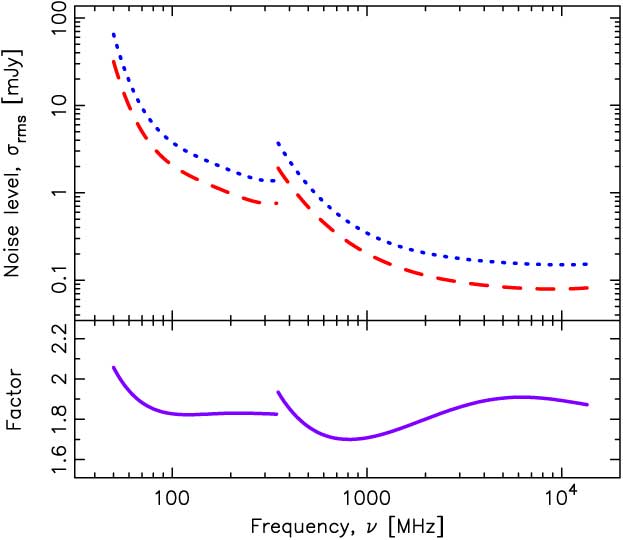
Figure 11. The noise level per each 10 km s−1 channel after 1 h of integration with the SKA1. The dotted curve shows the natural weighted array sensitivities (Figure 10) and the broken curve the expected sensitivities (Tables 1 and 2 of Braun Reference Braun2017). The bottom panel shows the ratio, i.e. the fudge factor in the noise level.
Inserting the values for A eff/T sys into Equation (1) and scaling by the fudge factor gives σ rms = 0.5 – 1.2 and 0.03 – 0.06 mJy per 10 km s−1 for phase-1 and phase-2, respectively. For the estimated flux densities, these result in (1/T spin)(d abs/d QSO)2 ∼ 10−3 K−1 and (1/T spin)(d abs/d QSO)2 ∼ 10−4 K−1 at z abs ≳ 3.5, respectively (Figure 12). We see that these limits approach those required to confirm the downturn in (1/T spin)(d abs/d QSO)2, particularly for the SKA phase-2. Examining this in detail, in Figure 13 we show the integration times required to reach the necessary sensitivities at z ≳ 3.5. From this, we see that most of the absorbers can be searched to sufficiently deep limits within a total of ∼ 1 000 h. Since we used the longest integration required along the sight-lines with multiple absorbers, we expect a number of observations to be significantly more sensitive than required. Furthermore, if the fraction of cool gas, as traced by (1/T spin)(d abs/d QSO)2, does not follow the same steep decline as the star formation density (Figure 1) at high redshift, we may expect detections within much shorter integration times. The wide SKA-low field-of-view will allow this time to be cut further by observing multiple sight-lines simultaneously (Figure 14), which, given the high sky density of DLAs (figure inset), will yield radio flux measurements (rather than estimates, 3.2), at 7″ resolution (Dewdney Reference Dewdney2015), and, possibly, unexpected 21-cm absorption.
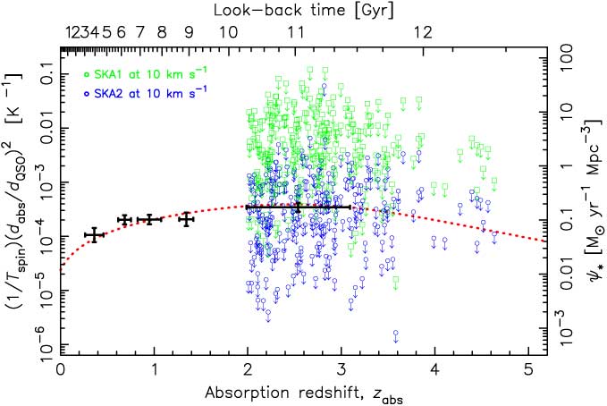
Figure 12. As Figure 6, but showing the limits reached by the SKA after 10 h of integration at 10 km s−1 per channel for sight-lines at δ < 29° (where 237 absorbers reach elevations of > 30°).
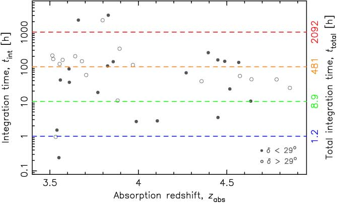
Figure 13. The integration times expected by the SKA2-low to obtain a 3σ detection if ψ * T spin (d QSO/d abs)2 = 500 M⊙ yr−1 Mpc−3 K (e.g. the dotted trace in Figure 12). The filled symbols show the sources at declinations of δ < 29° and the unfilled those with δ > 29°, although all of the targets have δ ≤ 41.8°. The right axis shows the total integration time required on the basis of the longest single integration for that sight-line. For example, restricting all targets to t int < 100 h gives 21 absorbers along 16 sight-lines with z abs > 3.5, for a total observing time of 481 h.
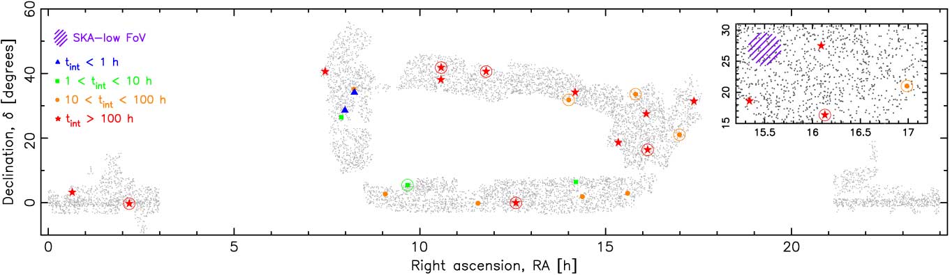
Figure 14. The sky distribution of the known radio-illuminated z abs > 3.5 absorbers. The shapes designate the maximum required integration time (see Figure 13) with those circled having more than one absorber at z abs > 3.5 along the sight-line. The small markers show the positions of the DR9 DLAs and the hatched region the SKA-low field-of-view (21 deg2, Dewdney Reference Dewdney2015). The inset shows a region of relatively high DLA density.
Looking further, several thousand 21-cm absorbers are expected to be detected with the SKA phase-1 at z abs ≲ 3, with no estimate for the numbers at high redshift (Morganti, Sadler & Curran Reference Morganti, Sadler and Curran2015; Allison et al. Reference Allison, Zwaan, Duchesne and Curran2016). Even in the absence of further large DLA catalogues, blind surveys with the SKA are expected to yield a large number of redshifted absorption systems which are dust reddened (Webster et al. Reference Webster, Francis, Peterson, Drinkwater and Masci1995; Carilli et al. Reference Carilli, Menten, Reid, Rupen and Yun1998; Curran et al. Reference Curran, Whiting, Allison, Tanna, Sadler and Athreya2017) and thus missed by those pre-selected based upon their optical/UV spectrum. The lack of an optical spectrum does, of course, prevent the nature of the absorber being determined—whether it arises in a quiescent galaxy, intervening a more distant continuum source (as per the DLAs), or is associated with the host of the background continuum source itself. Machine learning techniques do, however, offer the possibility of determining the nature of the absorber purely from its 21-cm absorption profile (Curran et al. Reference Curran, Duchesne, Divoli and Allison2016b). The other issue with avoiding optical pre-selection is the lack of a Lyman-α spectrum from which to determine the total neutral hydrogen column density. A statistical value for use in Equation (5) may, however, be derived from the cosmological HI density (Curran Reference Curran2017b).
4. Discussion and summary
It is now well established that the evolution of the mass density of neutral hydrogen is in stark disagreement to that of the star formation density. There is, however, recent compelling evidence that the fraction of cool gas, as traced through the HI 21-cm absorption strength normalised by the total column density, could trace ψ *. However, the paucity of 21-cm absorption searches at z abs ≳ 3.5 prevents us from confirming whether the cold gas fraction follows the same downturn as the star formation density. In this paper, we examine the possibility of testing this through observations of a large sample of damped Lyman-α absorption systems, the SDSS SDSS-III DR9 catalogue (Noterdaeme et al. Reference Noterdaeme2012). For each of the 12 081 N HI ≥ 1 ×1020 cm−2 absorption systems,
We search each sight-line in the NVSS, FIRST, and SUMSS for background radio emission. This yields 336 radio-loud sight-lines, containing a total of 414 absorbers. For each of these we obtain all of the available radio photometry and use this to estimate the flux density at the redshifted 21-cm frequency of each absorber.
For each of the current large radio interferometers, we determine which absorbers are redshifted into an available band and is visible from the telescope location.
From the instrument specifications, we calculate the sensitivity after a 10-h integration which we combine with the flux density and the neutral hydrogen column density, as well as removing line-of-sight geometry effects, to estimate the best expected limit to the spin temperature (degenerate with the ratio of the emitter–absorption extents) obtainable for each absorber.
From this, we find that none of the current instruments are of sufficient sensitivity to place useful limits on (1/T spin)(d abs/d QSO)2 at z abs ≳ 3.5, although both the upgraded (u)GMRT and (E)VLA may be sufficiently sensitive at 3 ≲ z abs ≲ 3.5. This, of course, does not preclude the possibility that a number of detections at these redshifts could rule out the hypothesis that ψ * is traced by(1/T spin)(d abs/d QSO)2, a possibility which can only be addressed through observation.
With the SKA, the required sensitivity is achievable at z abs ≳ 3.5, but only for a small number (≈ 10) of absorbers. This is due to the sensitivity function of the SDSS, exhibiting a steep decline in the number of sight-lines at z abs ≳ 3 (λobs ≳ 5000 Å, Noterdaeme et al. Reference Noterdaeme, Petitjean, Ledoux and Srianand2009, Reference Noterdaeme2012), above which the Lyman-α transition is shifted out of the optical and into the near-infrared band (at z abs ≳ 5.5). If our derived radio fluxes are representative at these redshifts, in addition to new DLAs found through further optical surveys over the next decade, we expect an increased number of absorbers to be detected through the wide instantaneous bandwidth and field-of-view of the SKA. The detection of new absorption systems in radio surveys would not be subject to the same dust obscuration as their optical counterparts. In the absence of an optical spectrum, it may be possible to determine whether the absorption is intervening or associated, through machine learning techniques (Curran et al. Reference Curran, Duchesne, Divoli and Allison2016b), and apply a statistical column density in order to yield a statistical (1/T spin)(d abs/d QSO)2 (Curran Reference Curran2017b).
Radio selection may also uncover intervening absorbers rich in molecular gas: although molecular absorption has been detected in 26 DLAs, through H2 vibrational transitions redshifted into the optical band at z abs ≳ 1.7 (compiled in Srianand et al. Reference Srianand, Gupta, Petitjean, Noterdaeme and Ledoux2010 with the addition of Reimers et al. Reference Reimers, Baade, Quast and Levshakov2003; Fynbo et al. Reference Fynbo2011; Guimarães et al. Reference Guimarães, Noterdaeme, Petitjean, Ledoux, Srianand, López and Rahmani2012; Srianand et al. Reference Srianand, Gupta, Petitjean, Noterdaeme, Ledoux, Salter and Saikia2012; Noterdaeme et al. Reference Noterdaeme, Srianand, Rahmani, Petitjean, Pâris, Ledoux, Gupta and López2015, Reference Noterdaeme2017; Balashev et al. Reference Balashev2017), extensive millimetre-wave observations have yet to detect absorption from any rotational transition (e.g. Curran et al. Reference Curran, Murphy, Pihlström, Webb, Bolatto and Bower2004b). Since the DLAs in which H2 has been detected have molecular fractions  ${\cal F} \equiv 2{N_{{{\rm {H}}_2}}}/(2{N_{{{\rm {H}}_2}}} + {N_{{\rm {H1}}}}) \sim {10^{ - 7}} - 0.3$ and optical—near-infrared colours of V – K ≲ 4 (Curran et al. Reference Curran2011), compared to the five known redshifted radio-band absorbers, where ℱ ≈ 0.7 – 1.1 and V – K ≥ 4.80 (Curran et al. Reference Curran, Whiting, Murphy, Webb, Longmore, Pihlström, Athreya and Blake2006), we suspect that the selection of optically bright objects selects against dusty environments, which are more likely to harbour molecules in abundance. Thus, radio-selected surveys offer the possibility of finally detecting dust obscured DLAs which have similarly high molecular fractions (ℱ ∼ 1). Comparison of the atomic and molecular line strengths will provide an invaluable probe of the conditions in the highest redshift galaxies. Furthermore, comparison of the relative shifts of the atomic and molecular transitions in the radio-band offers a measure of the fundamental constants of nature at large-look back times to much greater precision than optical spectroscopy (e.g. Murphy, Webb & Flambaum Reference Murphy, Webb and Flambaum2003; Tzanavaris et al. Reference Tzanavaris, Murphy, Webb, Flambaum and Curran2007), making the SKA ideal in resolving this contentious issue (Curran, Kanekar & Darling Reference Curran, Kanekar and Darling2004).
Acknowledgements
I wish to thank the referee for their very helpful comments, as well as James Allison and Randall Wayth for their help with the MWA specifications, Raymond Oonk, Vanessa Moss, and Antonis Polatidis for the LOFAR specifications and Robert Braun for the SKA specifications. This research has made use of the NASA/IPAC Extragalactic Database (NED) which is operated by the Jet Propulsion Laboratory, California Institute of Technology, under contract with the National Aeronautics and Space Administration and NASA’s Astrophysics Data System Bibliographic Service. This research has also made use of NASA’s Astrophysics Data System Bibliographic Service and ASURV Rev 1.2 (Lavalley, Isobe, & Feigelson Reference Lavalley, Isobe and Feigelson1992), which implements the methods presented in Isobe, Feigelson, & Nelson (Reference Isobe, Feigelson and Nelson1986).