2.1. Simulation of supersonic turbulent boundary layers

We first introduce the governing equations and the numerical settings for the fluid phase. The compressible turbulent boundary layer flows are governed by the three-dimensional Navier–Stokes equations for Newtonian perfect gases, cast as

(2.1)$$\begin{gather} \frac{\partial \rho}{\partial t} +\frac{\partial (\rho u_i)}{\partial x_i} = 0, \end{gather}$$

(2.2)$$\begin{gather}\frac{\partial (\rho u_i)}{\partial t} +\frac{\partial (\rho u_i u_j)}{\partial x_j} ={-}\frac{\partial p}{\partial x_i} + \frac{\partial \tau_{ij}}{\partial x_j}, \end{gather}$$

(2.3)$$\begin{gather}\frac{\partial (\rho E)}{\partial t} +\frac{\partial (\rho E u_j)}{\partial x_j} ={-}\frac{\partial (p u_j)}{\partial x_j} + \frac{\partial (\tau_{ij} u_i)}{\partial x_j} -\frac{\partial q_j}{\partial x_j}, \end{gather}$$

where $u_i$ is the velocity component of the fluid in the $x_i$ direction, with $i=1,2,3$ (also $x$, $y$ and $z$) denoting the streamwise, wall-normal and spanwise directions. Here, $\rho$ is density, $p$ is pressure, and $E$ is total energy, related by the following state equations of perfect gases:

(2.4a,b)\begin{equation} p=\rho R T,\quad E=C_v T + \tfrac{1}{2} u_i u_i, \end{equation}

where $T$ is temperature, $R$ is the gas constant, and $C_v$ is the constant volume specific heat. The viscous stresses and the molecular heat conductivity are determined by the following constitutive equations for Newtonian fluids and Fourier's law, respectively:

(2.5a,b)\begin{equation} \tau_{ij}= \mu \left( \frac{\partial u_i}{\partial x_j}+\frac{\partial u_j}{\partial x_i} \right) -\frac{2}{3}\,\mu\,\frac{\partial u_k}{\partial x_k}\,\delta_{ij},\quad q_j ={-} \kappa\, \frac{\partial T}{\partial x_j}, \end{equation}

where $\mu$ is the viscosity, calculated by Sutherland's law, and $\kappa$ is the molecular heat conductivity, determined as $\kappa = C_p \mu /Pr$.

The DNS are performed utilizing the open-source code STREAmS developed by Bernardini et al. (Reference Bernardini, Modesti, Salvadore and Pirozzoli2021), using the finite difference method to solve the governing equations. The convective terms are approximated by the sixth-order kinetic energy preserving scheme (Kennedy & Gruber Reference Kennedy and Gruber2008; Pirozzoli Reference Pirozzoli2010) in the smooth region and the fifth-order weighted essentially non-oscillation (WENO) scheme (Shu & Osher Reference Shu and Osher1988) when the flow discontinuity is detected by the Ducros sensor (Ducros et al. Reference Ducros, Ferrand, Nicoud, Weber, Darracq, Gacherieu and Poinsot1999). The viscous terms are approximated by the sixth-order central scheme. The low-storage third-order Runge–Kutta scheme is adopted for time advancement (Wray Reference Wray1990).

The boundary conditions are given as follows. The turbulent inlet is composed of the mean flow obtained by empirical formulas (Musker Reference Musker1979) and the synthetic turbulent fluctuations using the digital filtering method (Klein, Sadiki & Janicka Reference Klein, Sadiki and Janicka2003). The no-reflecting conditions are enforced at the upper and outlet boundaries. Periodic conditions are adopted in the spanwise direction. The no-slip condition for velocity and the isothermal condition for temperature are given at the lower wall.

Herein, the free stream flow parameters are denoted by the subscript $\infty$. The free stream Mach number is defined as the ratio between the free stream velocity and the sound speed $M_\infty = U_\infty / \sqrt {\gamma R T_\infty }$, and the free stream Reynolds number is defined as $Re_\infty = \rho _\infty U_\infty \delta _0/\mu _\infty$, with $\delta _0$ the nominal boundary layer thickness at the turbulent inlet. The ensemble average of a generic flow quantity $\varphi$ is marked as $\bar \varphi$, the corresponding fluctuations as $\varphi '$, the density-weighted average (Favre average) as $\tilde \varphi$, and the corresponding fluctuations as $\varphi ''$. The viscous scales are defined based on the mean shear stress $\tau _w$, viscosity $\mu _w$, and density $\rho _w$ at the wall, resulting in the friction velocity $u_\tau =\sqrt {\tau _w/\rho _w}$, viscous length scale $\delta _\nu = \mu _w / (\rho _w u_\tau )$ and friction Reynolds number $Re_\tau = \rho _w u_\tau \delta /\mu _w$ (with $\delta$ the nominal boundary layer thickness at a given streamwise station). The flow quantities normalized by these viscous scales are denoted by the superscript $+$. Local viscous scales are defined accordingly by substituting the wall density $\rho _w$ and wall viscosity $\mu _w$ with their local mean values, and the flow quantities normalized by these local viscous scales are marked by the superscript $*$.

The streamwise, wall-normal and spanwise sizes of the computational domain are set as $L_1=80 \delta _0$, $L_2 = 9 \delta _0$ and $L_3 = 8 \delta _0$, discretized by $2400$, $280$ and $280$ grids, respectively. The grids are distributed uniformly in the streamwise and spanwise directions, and stretched by a hyperbolic sine function in the wall-normal direction, with $240$ grids clustered below $y= 2.5 \delta _0$. At the inlet, the friction Reynolds number is set as $Re_{\tau 0} = 200$, according to which the free stream Reynolds number $Re_\infty$ is calculated. The streamwise and spanwise grid intervals defined based on the viscous scales at the turbulent inlet are $\Delta x^+ = 6.67$ and $\Delta z^+ = 5.71$. The first grid off the wall is located at $\Delta y^+_w=0.5$, and the grid interval in the free stream is $\Delta y^+=7.06$. Such grid intervals are sufficient with the presently used low-dissipative numerical schemes (Pirozzoli Reference Pirozzoli2011).

The free stream Mach numbers of the turbulent boundary layers are set as $M_\infty = 2$, 4 and 6. The wall temperatures $T_w$ are set to be constant values equal to the recovery temperature $T_r = T_\infty (1+(\gamma -1) r M^2_\infty )/2$, the mean wall temperature with adiabatic conditions at the given Mach number, with $\gamma =1.4$ the specific heat ratio, $r=Pr^{1/2}$ the recovery factor, and $Pr=0.71$ the Prandtl number. The streamwise variation of the nominal ($Re_\delta$), displacement ($Re_{\delta ^*}$), momentum ($Re_\theta$) and friction ($Re_\tau$) Reynolds numbers in the statistically equilibrium regions are listed in table 1. Although the ranges of $Re_\delta$, $Re_{\delta ^*}$ and $Re_\theta$ are different at various Mach numbers, the friction Reynolds numbers $Re_\tau$ are of the same level, which is the most important parameter in wall-bounded turbulence. Hereinafter, the results reported are obtained within the streamwise range $(60\unicode{x2013} 70) \delta _0$ and the time span $240 \delta _0/U_\infty$ to obtain converged statistics. The data are not collected until the simulations have been run for $1000 \delta _0/U_\infty$, during which the turbulent flows are fully developed and the distributions of particles in the wall-normal direction reach steady states, as we will demonstrate subsequently.

Table 1. Flow parameters. Here, $Re_\delta$, $Re_\delta ^*$ and $Re_\theta$ are the Reynolds numbers defined by the nominal ($\delta$), displacement ($\delta ^*$) and momentum ($\theta$) boundary layer thicknesses.

In figure 1(a) we present the van Driest transformed mean velocity obtained by the integration

(2.6)\begin{equation} u^+_{1,VD} = \frac{1}{u_\tau} \int^{\bar u_1}_0 \left( \frac{\bar \rho}{\bar \rho_w} \right)^{1/2} {\rm d} u_1, \end{equation}

along with values reported by Bernardini & Pirozzoli (Reference Bernardini and Pirozzoli2011) at $M_\infty =2$ and $Re_\tau \approx 450$ for comparison. For all the cases considered, the van Driest transformed mean velocity profiles are well collapsed and consistent with the reference data below $y^+=100$, obeying the linear law in the viscous sublayer, and the logarithmic law in the log region (if any). The disparity in the wake region can be ascribed to the slightly lower friction Reynolds number $Re_\tau$ in the present study. The mean temperatures $\bar T$ are shown in figure 1(b), manifesting zero gradients close to the wall due to the quasi-adiabatic thermal condition and monotonic decrement as it approaches the outer edge of the boundary layer. The mean temperature profiles are well collapsed with the generalized Reynolds analogy proposed by Zhang et al. (Reference Zhang, Bi, Hussain and She2014) that relates the mean temperature and the mean velocity:

(2.7)\begin{equation} \frac{\bar T}{T_\infty} = \frac{T_w}{T_\infty} + \frac{T_{rg}-T_w}{T_\infty}\,\frac{\bar u}{U_\infty} +\frac{T_\infty-T_{rg}}{T_\infty} \left( \frac{\bar u}{U_\infty} \right)^2,\end{equation}

where $T_{rg}$ is the generalized total temperature

(2.8)\begin{equation} T_{rg} = T_\infty + r_g\,\frac{U^2_\infty}{2C_p}, \end{equation}

with $r_g$ the generalized recovery coefficient.

Figure 1. Wall-normal distributions of (a) van Driest transformed mean velocity $u^+_{1,VD}$, (b) mean temperature $\bar T/T_\infty$, (c,d) Reynolds stresses $R^+_{ij}$. Blue dash-dotted lines indicate case M2; red dashed lines indicate case M4; black solid lines indicate case M6. Grey lines in (a) indicate logarithmic law $2.44 \ln (y^+) + 5.2$. Symbols in (a,c,d) indicate reference data from Bernardini & Pirozzoli (Reference Bernardini and Pirozzoli2011) at $M_\infty =2$ and $Re_\tau \approx 450$; symbols in (b) indicate mean temperature obtained by the generalized Reynolds analogy.

Figures 1(c) and 1(d) display the distributions of the Reynolds stresses $R^+_{ij} = \overline {\rho u''_i u''_j}/\tau _w$ for the three cases, amongst which those of case M2 show agreement with the reference data reported by Bernardini & Pirozzoli (Reference Bernardini and Pirozzoli2011) in the near-wall region when plotted against the viscous coordinate (figure 1c), and also in the outer region when plotted against the global coordinate (figure 1d), except for the slightly lower peaks of $R^+_{11}$ due to the lower Reynolds number. The Reynolds stresses are weakly dependent on the Mach number, showing a slight increment of the inner peaks with the Mach number. This is consistent with the previous studies of Cogo et al. (Reference Cogo, Salvadore, Picano and Bernardini2022) and Yu, Xu & Pirozzoli (Reference Yu, Xu and Pirozzoli2019).

2.2. Particle simulations in the Lagrangian framework

The dispersed phase considered herein is composed of heavy spherical particles with infinitesimal volume and mass fractions, thereby disregarding the inter-particle collisions and the feedback effects from the particles to the fluid (Kuerten Reference Kuerten2016). In the one-way coupling approximation, the trajectories and the motions of the spherical particles are solved by the equations

(2.9a,b)\begin{equation} \frac{{\rm d} r_{p,i}}{{\rm d}t} = v_i,\quad \frac{{\rm d} v_{i}}{{\rm d}t} = a_i, \end{equation}

with $r_{p,i}$, $v_i$ and $a_i$ denoting the particle position, velocity and acceleration. We consider merely the Stokes drag force induced by the slip velocity, while neglecting the other components such as the lift force, Basset history force and virtual mass force due to the large density of particles compared with that of the fluid (Maxey & Riley Reference Maxey and Riley1983; Armenio & Fiorotto Reference Armenio and Fiorotto2001; Mortimer et al. Reference Mortimer, Njobuenwu and Fairweather2019), cast as

(2.10)\begin{equation} a_i = \frac{f_{D}}{\tau_p}\,(u_i-v_i),\end{equation}

where $\tau _p = \rho _p d^2_p/18 \mu$ is the particle relaxation time, $d_p$ is the particle diameter, and $\rho _p$ is the particle density. The coefficient $f_D$ is estimated as

(2.11)$$\begin{gather} f_D = (1+0.15\,Re^{0.687}_p) H_M, \end{gather}$$

(2.12)$$\begin{gather}H_M = \begin{cases} 0.0239 M^3_p + 0.212 M^2_p - 0.074 M_p + 1, & M_p \le 1, \\ 0.93 + \dfrac{1}{3.5 + M^5_p}, & M_p >1 \end{cases} \end{gather}$$

incorporating the compressibility effects, as suggested by Loth et al. (Reference Loth, Tyler Daspit, Jeong, Nagata and Nonomura2021), with $Re_p = \rho \,|u_i - v_i|\,d_p/\mu$ and $M_p = |u_i - v_i|/\sqrt {\gamma R T}$ being the particle Reynolds and Mach numbers, respectively. Note that we have neglected the rarefied effects, for according to a preliminary estimation and the DNS results, particle Knudsen numbers rarely reach higher than 0.01, the criterion where the rarefied effects should be taken into account. The high Reynolds number modification incorporating the effects of the fully turbulent wake (Clift & Gauvin Reference Clift and Gauvin1971) has also been disregarded, for the particle Reynolds numbers are always lower than $100$.

We adopt the same strategy in the time advancement of the particle equations as the fluid phase using the third-order low-storage Runge–Kutta scheme. Trilinear interpolation is used to obtain information about the fluid at the particle position (Eaton Reference Eaton2009; Bernardini Reference Bernardini2014). We performed DNS of particles in turbulent channel flows for validation; for details, refer to Appendix A. The initial positions of the particles in the simulation are distributed randomly within $y=2 \delta _0$, with their initial velocities set to be the same as those of the fluid. The perfectly elastic collisions are assumed when the particles hit the wall. Periodic conditions are imposed as in the fluid phase in the spanwise direction. When the particles pass through the upper boundary and the flow outlet, they are recycled to the flow inlet with a random wall-normal and spanwise position below $y=\delta _0$, and the same velocity as that of the fluid at that location so as to retain the total number of particles. As mentioned in the previous subsection, the flow statistics reported hereinafter are obtained within the range $(60 \unicode{x2013}70) \delta _0$, where the particle fields are considered to be fully developed, with the validation presented in Appendix B.

The dispersed phase contains seven particle populations with the same particle numbers $N_p = 10^6$. As reported in table 2, these particle populations share the identical diameter $d_p=0.001 \delta _0$ and various density ratios $\rho _p / \rho _\infty$ ranging from 20 to 50 000. Within the nominal boundary layer thickness, the volume fraction of the dispersed particle phase is approximately $4\times 10^{-7}$, and the mass fraction ranges from $8 \times 10^{-6}$ to $0.02$, suggesting the appropriateness of the one-way coupling approximation. In figure 2(a), we present the ratios between the particle diameter and the Kolmogorov scale $d_p/\eta$, which are lower than $1.0$ across the boundary layer, satisfying the requirements of the point-particle approach (Maxey & Riley Reference Maxey and Riley1983; Kuerten Reference Kuerten2016). When normalized by the local viscous length scale, as shown in figure 2(b), the particle diameters $d^*_p$ are approximately $0.185$ at the wall and increase monotonically towards the edge of the boundary layer, with the highest value $4.734$ at $M_\infty =6$.

Table 2. Particle diameters, density ratios and Stokes numbers.

Figure 2. Wall-normal distribution of the particle diameters (a) $d_p/\eta$ and (b) $d^*_p$, and the relative particle Stokes numbers (c) $St_K/St_{Kw}$ and (d) $St^*/St^+$. Blue dash-dotted lines indicate case M2; red dashed lines indicate case M4; black solid lines indicate case M6.

The different particle densities lead to the disparity in the particle relaxation time $\tau _p$. In table 2, we list three sets of particle Stokes numbers,

(2.13a–c)\begin{equation} St_\infty = \tau_p / \tau_\infty,\quad St^+{=} \tau_p / \tau_\nu,\quad St_{K,w} = \tau_p / \tau_{K,w}, \end{equation}

representing the ratio between the particle relaxation time $\tau _p$ and the characteristic time scale of the flow under the outer scale $\tau _\infty = \delta _0 / U_\infty$, under the viscous scale $\tau _\nu = \delta _\nu / u_\tau$, and under the Kolmogorov scale at the wall $\tau _{K,w} = (\mu _w/\varepsilon _w)^{1/2}$. Amongst these parameters, $St_{K,w}$ is a crucial parameter in isotropic turbulence, determining the features of the particle dynamics and accumulation (Balachandar & Eaton Reference Balachandar and Eaton2010; Brandt & Coletti Reference Brandt and Coletti2022), whereas $St^+$ is commonly used in wall turbulence. For particles in incompressible wall turbulence without viscosity stratification, both $\tau _p$ and $\tau _\nu$ are constant. However, this is not the case for the presently considered flow, for the viscosity $\mu$ is a function of temperature, complicating the evaluation of the particle inertia. In figures 2(c,d), we present the distributions of $St_K$ and $St^+$ compared with their values at the wall. Due to the lower dissipation, $St_K$ decreases monotonically away from the wall, showing weak Mach number dependence. The $St^*$ values, on the other hand, increase with the wall-normal coordinate, and escalate with the Mach number, indicating that the response of the particle to the turbulent fluctuation of the fluid flow is varying across the boundary layer due to the stratification of the mean density and viscosity, especially near the edge of the boundary layer.

3.1. Instantaneous particle distribution

We first present in figure 3 the instantaneous distribution of the particle populations P1, P4, P5 and P6, and the fluid density $\rho$ in case M4, along with the edge of the boundary layer marked by $u_1 = 0.99 U_\infty$. For population P1, with the lowest particle density $\rho _p$ and Stokes number $St^+$, the particles appear to be uniformly distributed within the region where the fluid density is lower than that of the free stream value, even inside the small ‘blobs’ that are spatially separated from the turbulent boundary layer, but fail to fill in the regions between these ‘blobs’ and the primary turbulent regions of the boundary layers, the region where the density is the free stream value but the momentum is lower. As the Stokes number increases to $St^+ \approx 17.6$ (P4) and $70.44$ (P5), the particles accumulate close to the wall, thereby leading to their lower concentration at higher locations. Due to their comparatively larger inertia away from the wall (recall figure 2d), some of the particles with high vertical velocities are capable of escaping from the low-fluid-density regions and reaching the free stream. This is especially the case for population P6 ($St^+ \approx 140.81$) with an even larger particle density, a considerable portion of which can be ejected to the free stream, while the tendency of wall accumulation is weakened. The variation of the particle distributions with the Stokes numbers in other flow cases is similar to this case, showing non-monotonic behaviour of near-wall accumulation. This is consistent with previous studies in incompressible wall turbulence (Marchioli & Soldati Reference Marchioli and Soldati2002; Bernardini Reference Bernardini2014).

Figure 3. Instantaneous density distribution at $z=0$ (flooded) and particles within $z=0\unicode{x2013} 0.01 \delta _0$ in case M4, for particle populations (a) P1, (b) P4, (c) P5, (d) P6. Black solid lines indicate $u_1 = 0.99 U_\infty$.

We would like to remark on the resemblance in the instantaneous distributions of the low Stokes number particles and the fluid density. It has been shown that in the limit of small volumetric loading, the concentration field $c$ (number of particles per volume) of the particles can be approximated as (Ferry & Balachandar Reference Ferry and Balachandar2001, Reference Ferry and Balachandar2002)

(3.1)\begin{equation} \frac{\partial c}{\partial t} + \frac{\partial c v_j}{\partial x_j} = c\,\frac{\partial u_i}{\partial x_i}. \end{equation}

Under the conditions $\rho _p / \rho _f \gg 1$ and $St^+ \ll 1$, the velocities of the fluid and particles are approximately the same, $v_i \approx u_i$, with the deviation being of the order of $O(\tau _p)$ in outer scales. For the presently considered compressible flow over a quasi-adiabatic flat plate, the flow dilatation can be disregarded in comparison with the vortical and shear (Yu et al. Reference Yu, Xu and Pirozzoli2019; Yu & Xu Reference Yu and Xu2021), so the right-hand side of (3.1) can be neglected, leading to the identical expression of (3.1) and the continuity equation. It is therefore reasonable that the density and the low Stokes number particle concentration fields are similar, except that there are mean gradients in the fluid density due to the restriction of the state equation of the perfect gas and the non-uniformity of the mean temperature in the wall-normal direction.

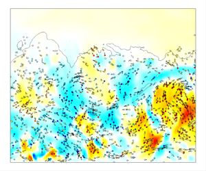
To further characterize the wall-normal transport of the particles, in figure 4 we present the wall-normal velocity of the fluid and the in-plane particle velocity vectors. For population P1, the wall-normal velocities of these low Stokes number particles follow almost exactly that of the fluid, in that the particles are moving upwards in the regions of ejections and downwards in the regions of sweeps within the boundary layer. However, near the edge of the boundary layer, the particles prefer to accumulate by the strong ejections, as suggested by higher particle concentration within the regions of positive wall-normal velocity $u_2>0$ compared to those of the negative wall-normal velocity $u_2<0$. This has been examined via probability density distributions, as demonstrated in Appendix C. A simple reason is that there is no particle outside the boundary layers, so no particle can be brought downwards into the turbulent boundary layers from the free stream flow. This will be reflected in the statistics of particles as well, as will be shown subsequently. As for the other particle populations with larger Stokes numbers $St^+$, their wall-normal transport processes are still approximately following those of the fluid, while the magnitudes are reduced due to the larger particle inertia. In spite of this, the particles are more inclined to move outwards to the free stream, even inside $u_2<0$ regions, which is probably the remnant of the strong ejection events or equivalently the historical effects of the large-inertia particles (Soldati Reference Soldati2005). However, it should be noted that the number of particles escaping the turbulent boundary layers does not increase monotonically with the Stokes number. On the one hand, it can be derived that in the comparatively quiescent flow, the initial slip velocity required for the particles to reach the free stream is proportional to the reciprocal of the Stokes number. Henceforth, the high Stokes number particles are capable of escaping the boundary layers even though their wall-normal velocities are generally small. On the other hand, the bursting events endowed with high-intensity vertical momentum are usually short-lived (Tardu Reference Tardu1995; Jiménez Reference Jiménez2013, Reference Jiménez2018), so it is unlikely that the extremely high Stokes number particles can be accelerated to the threshold of escaping the boundary layer. Subject to these counteracting factors, the number of particles reaching the free stream should be first increasing then diminished, and when the Stokes numbers are sufficiently large, recovers to zero, for the particles will remain an almost straight trajectory with slight influences by the turbulent motions.

Figure 4. Instantaneous wall-normal velocity of the fluid $u_2$ (flooded) at $x=60 \delta _0$ and particle distribution within $x=(60\unicode{x2013}60.01) \delta _0$ in case M4, for (a) P1, (b) P4, (c) P5, (d) P6. Arrows indicate in-plane particle velocity vectors.

In figure 5, we present the distribution of the streamwise velocity fluctuation $u'_1$ at $y^+=15$ and the particles within the range $y^+=3\unicode{x2013}15$. As is commonly observed in dilute multi-phase wall turbulence (Rouson & Eaton Reference Rouson and Eaton2001; Sardina et al. Reference Sardina, Schlatter, Brandt, Picano and Casciola2012; Bernardini et al. Reference Bernardini, Pirozzoli and Orlandi2013), the particles with low $St^+$ are evenly distributed in the wall-parallel plane, while their clustering with the low-speed streaks can be spotted for moderate $St^+$ particles (populations P4 and P5), which is induced by the near-wall quasi-streamwise vortices that transport the particles towards the viscous sublayer and are deposited by the spanwise velocity below the low-speed streaks, where they are either trapped or brought upwards when encountered with the strong ejections (Marchioli & Soldati Reference Marchioli and Soldati2002; Soldati & Marchioli Reference Soldati and Marchioli2009). At larger $St^+$ in type P6, the ‘particle streaks’ are weakened, showing a more uniform distribution, which is caused by the highly different particle response time and characteristic time scale of the near-wall self-sustaining cycle. Much longer particle streaks with wider spanwise intervals will be observed in high Reynolds number flows in which the very-large-scale motions are becoming more and more manifest, and contribute significantly to the Reynolds stress (Jie et al. Reference Jie, Cui, Xu and Zhao2022; Motoori et al. Reference Motoori, Wong and Goto2022).

Figure 5. Instantaneous streamwise velocity fluctuation $u'_1$ at $y^+=15$ (flooded) and particle distribution within $y^+=3\unicode{x2013}15$ in case M4, for (a) P1, (b) P4, (c) P5, (d) P6.

3.2. Near-wall accumulation and clustering

The non-uniform wall-normal distribution can be characterized quantitatively by the mean particle concentration, calculated based on the grid centre of the Eulerian frame as

(3.2) \begin{equation} c(y_j) = \frac{N_p(y_j)}{\displaystyle\sum\nolimits_{j} N_p(y_j)}\, \displaystyle\frac{\displaystyle\sum\nolimits_{j} \Delta h_j}{\Delta h_j},\quad j=1, 2,\ldots, N_y-1, \end{equation}

where $N_p (y_j)$ is the particle number located between the $j$th and $(j+1)$th grid points, and $\Delta h_j$ is the grid interval. The distributions of the mean particle concentration $\bar c(y)/c_0$ are displayed in figures 6(a–c), with $c_0$ the particle concentration in the case of the perfect uniform wall-normal distribution. In general, the particles are almost evenly distributed across the boundary layer for the populations with the lowest Stokes number $St^+$, and the phenomenon of the near-wall accumulation, namely the turbophoresis, becomes more evident with increasing $St^+$. The maximal near-wall particle number density is attained for the particle type P4, beyond which it is gradually diminished. This is consistent with the conclusions in low-speed turbulent channel flows (Sardina et al. Reference Sardina, Schlatter, Brandt, Picano and Casciola2012; Bernardini Reference Bernardini2014). Comparing these cases, we found that the particle concentrations $\bar c(y)$ within the range $y^+ = 50\unicode{x2013}200$ remain almost constant in case M2, whereas those in cases M4 and M6 slightly increase and manifest secondary peaks in the outer region, especially for the large $St^+$ particle populations. Such non-monotonic variations are probably caused by the evident variation of the particle Stokes number $St^*$ at high Mach numbers when evaluated by the local density and viscosity of the fluid.

Figure 6. Wall-normal distribution of the particle concentration in cases (a) M2, (b) M4 and (c) M6; and (d) the Shannon entropy at different Stokes numbers $St^+$ at $t=515 \delta _0/U_\infty$. Lines in (d) are the cubic splines using the data within $St^+ = 1 \unicode{x2013}300$.

A commonly used indicator of the non-uniform wall-normal distribution is the Shannon entropy (Picano, Sardina & Casciola Reference Picano, Sardina and Casciola2009). It is defined by the ratio of two entropy parameters, $S_p = \mathscr{S}/\mathscr {S}_{max}$, in which $\mathscr {S}$ is calculated in equidistant slabs in the wall-normal direction within $1.2 \delta$:

(3.3)\begin{equation} \mathscr{S} ={-} \sum^{N_{yu}}_{j=1} P_j \ln (P_j), \end{equation}

with $N_{yu}=200$, and $P_j$ the probability of finding a particle in the $j$th slab. In the case of evenly distributed particles, $\mathscr {S}$ attains a maximum $\mathscr {S}_{max}=\ln N_{yu}$. The Shannon entropy $S_p$ therefore ranges from 0 to 1. In figure 6(d), we plot the values of $S_p$ of each particle population in all three cases against $St^+$. As expected, the values of $S_p$ are close to unity for low Stokes number particles, corresponding to the uniform distribution across the boundary layer, and decrease rapidly and attain a minimum at $St^+ \approx 30$ for all the cases considered, irrespective of the free stream Mach numbers, suggesting the highest level of near-wall accumulation. This is consistent with previous studies on particles in incompressible turbulent channels (Marchioli & Soldati Reference Marchioli and Soldati2002; Bernardini Reference Bernardini2014). For particles with $St^+$ greater than $300$, the $S_p$ values tend to reach an asymptotic value $0.85$, implying that the tendency of near-wall accumulation of particles remains even when the particles respond to the turbulent motions rather slowly, which is probably caused by the integral effects of their remaining inside the turbulent boundary layer. Comparing the cases at different Mach numbers, we further found that the higher Mach numbers tend to alleviate the turbophoresis phenomenon. This can be inferred from the larger particle number density near the edge of the boundary layer. It is reminiscent of the higher particle concentration near the channel centre within the quiescent cores (Jie et al. Reference Jie, Andersson and Zhao2021) and the free surface of the open channel (Yu et al. Reference Yu, Lin, Shao and Wang2017; Gao, Samtaney & Richter Reference Gao, Samtaney and Richter2023), which was attributed to the corresponding lower turbulent intensities (Mortimer & Fairweather Reference Mortimer and Fairweather2020). Such a phenomenon is found to be more evident for larger Stokes number particles. Therefore, the more intense particle concentration near the edge of the boundary layer with increasing Mach number should probably be attributed to the larger $St^*$, as reported in figure 2(d).

Since the near-wall accumulation is related mainly to the ejection and sweeping events induced by the quasi-streamwise vortices (Marchioli & Soldati Reference Marchioli and Soldati2002; Soldati & Marchioli Reference Soldati and Marchioli2009), the dependence of the Shannon entropy on the Mach number is probably caused by the variation of the characteristics of the streamwise vortices. In figure 7, we present the root mean square (RMS) of the streamwise vorticity fluctuations, $\bar \omega '_x$, normalized by the viscous scales and local viscous scales, respectively. For the local peaks at $y^+ \approx 10\unicode{x2013}20$ that represent the average intensity of the quasi-streamwise vortices, the former shows weak dependence on the Mach number, while the latter manifests a systematic decreasing trend of variation. From another point of view, the normalization using the viscous scales is more of a kinetic description of the fluid motions, while that using the local viscous scales incorporates the variation of the fluid density and viscosity that influence the motions of the particles. Therefore, we conclude that the decreasing $\bar \omega '^*_x$ suggests the weaker impacts of the streamwise vortices on the near-wall particle motions, consistent with the observations of the less intensified near-wall accumulation with the Mach number.

Figure 7. Wall-normal distribution of the streamwise vorticity fluctuation root mean square, normalized by (a) viscous scale $\delta _\nu /u_\tau$, $\bar \omega '^+_x$, (b) local viscous scales $\delta ^*_\nu /u^*_\tau$, $\bar \omega '^*_x$. Blue dash-dotted lines indicate case M2; red dashed lines indicate case M4; black solid lines indicate case M6.

Besides the near-wall accumulation, another crucial aspect of the particle organization in wall turbulence is the clustering behaviour in the wall-parallel planes induced by the turbulent structures. Amongst the multiple methods of quantifying such a phenomenon, such as the maximum deviation from randomness or the segregation parameter (Fessler, Kulick & Eaton Reference Fessler, Kulick and Eaton1994; Picciotto et al. Reference Picciotto, Marchioli and Soldati2005b), the scaling of the radial distribution function (RDF) (Wang & Maxey Reference Wang and Maxey1993; Pumir & Wilkinson Reference Pumir and Wilkinson2016), the statistics of particle concentration and the Voronoï tessellation analysis (Monchaux, Bourgoin & Cartellier Reference Monchaux, Bourgoin and Cartellier2010, Reference Monchaux, Bourgoin and Cartellier2012), we adopt the angular distribution function (ADF) proposed by Gualtieri, Picano & Casciola (Reference Gualtieri, Picano and Casciola2009), which has been applied to turbulent channel flows in Sardina et al. (Reference Sardina, Schlatter, Brandt, Picano and Casciola2012) for the characterization of the inhomogeneous near-wall particle organization. Following Sardina et al. (Reference Sardina, Schlatter, Brandt, Picano and Casciola2012), we define the two-dimensional ADF as

(3.4)\begin{equation} g(r,\theta)=\frac{1}{r}\,\frac{{\rm d} \nu_r}{{\rm d} r}\,\frac{1}{n_0(y)}, \end{equation}

with $r$ the wall-parallel inter-particle distance, $\theta$ the deviation angle from the $x$ direction, $\nu _r (r, \theta )$ the averaged particle pair number at a certain off-wall distance $y$, and $n_0$ the total number of particle pairs per unit area obtained by

(3.5)\begin{equation} n_0(y)=\frac{1}{2A}\,N_p(y)\,(N_p(y)-1), \end{equation}

where $A$ is the wall-parallel area where the statistics are performed.

In figure 8, we present the ADF distributions for particle populations P2 to P7 in case M4. The trend of variation is qualitatively consistent with that in low-speed turbulent channels (Sardina et al. Reference Sardina, Schlatter, Brandt, Picano and Casciola2012). Specifically, the particle population P2 with $St^+$ closest to unity manifests the weakest degree of small-scale clustering and the general uniform distribution, as indicated by the merely slightly higher value of ADF at $r=0$ compared to those away from it, where they remain almost constant. For particle populations P3 to P5 with the gradually larger $St^+$, the probability of finding particles adjacent to them in the streamwise direction is higher, corresponding to the formation and the more evident streamwise elongated particle streaks. At the even larger $St^+$ for particle populations P6 and P7, the particle streaks still exist but become less evident due to the higher probability away from $l^+_z =0$. This is consistent with the observations in figure 5 that the particles tend to be uniformly distributed when their inertia is large.

Figure 8. Near-wall particle angular distribution function below $y^+=10$ of case M4, for (a) P2, (b) P3, (c) P4, (d) P5, (e) P6, (f) P7.

Integrating the ADF in the azimuthal direction, we can obtain its isotropic component without incorporating the directional variation, namely the RDF

(3.6)\begin{equation} g_0 (r) = \frac{1}{2 {\rm \pi}} \int^{2 {\rm \pi}}_0 g(r,\theta)\, {\rm d} \theta. \end{equation}

The results for cases M2, M4 and M6 are shown in figures 9(a–c). Here, $g_0 (r)$ characterizes the probability of finding particle pairs within the circle of radius $r$, suggesting the level of radial particle clustering. For the presently considered cases, particle populations P4 and P5 show the most evident tendency for clustering, while for the other particle populations, such an effect is alleviated. Comparing these cases, we found that the particles with the highest value of $g_0(r)$ at the limit $r \rightarrow 0$ share approximately the same particle inertia under wall viscous units, $St^+ \approx 15\unicode{x2013}50$.

Figure 9. Isotropic component of the ADF $g_0(r)$ below $y^+=10$, for (a) case M2, (b) case M4, (c) case M6; and (d) power law of $g_0(r)$ at $r \rightarrow 0$ against $St^+$.

The RDF $g_0 (r)$ is capable of reflecting the small-scale clustering (Bec et al. Reference Bec, Biferale, Cencini, Lanotte, Musacchio and Toschi2007; Saw et al. Reference Saw, Shaw, Ayyalasomayajula, Chuang and Gylfason2008), as suggested by its association with the number of particle pairs within radius $r$:

(3.7)\begin{equation} {\mathscr N}(r) = n_0 \int^{2{\rm \pi}}_0 \int^r_0 r'\, g(r',\theta) \,{\rm d} r \,{\rm d} \theta. \end{equation}

For the spatially uniformly distributed particles, ${\mathscr N}(r)$ can be estimated as ${\mathscr N}(r) = n_0 (y)\,{\rm \pi} r^2$, hence $g_0$ being constant, otherwise the decay of $g_0$ at the limit $r \rightarrow 0$ should follow $g_0 \propto r^{-\alpha }$ with $\alpha >0$. The exponents $\alpha$ in the power law for all the particle populations in each case are shown in figure 9(d), with cubic spline curve fitting using the data within the range $St^+ = 5\unicode{x2013}300$. It can be observed that the peaks of $\alpha$ are attained at $St^+ \approx 15\unicode{x2013}30$, and the tendency of small-scale clustering is mitigated by the higher Mach number. This is probably caused by the lower level of the near-wall particle accumulation at higher Mach numbers, which reduces the particle numbers close to the wall (figure 6d).

The anisotropy indicator of the particle clustering can be obtained by the ADF as (Casciola et al. Reference Casciola, Gualtieri, Jacob and Piva2007; Sardina et al. Reference Sardina, Schlatter, Brandt, Picano and Casciola2012)

(3.8)\begin{equation} A(r) = \sqrt{\frac{\displaystyle \int (g(r,\theta)-g_0(r))^2 \,{\rm d} \theta}{\displaystyle \int g^2_0(r) \,{\rm d} \theta}}, \end{equation}

indicating the directional non-homogeneity of the wall-parallel particle distribution. The results are shown in figures 10(a–c). For particles with small $St^+$ or those with $St^+$ greater than $200$, the values of $A(r)$ are small and decay almost monotonically with increasing $r^+$, suggesting the weak directional dependence of $g(r,\theta )$ and hence the uniform distribution in almost all directions. For other particle populations with $St^+$ ranging from $5.0$ to $200$, the levels of $A(r)$ are higher, and the peaks are attained not at the limit $r^+ \rightarrow 0$, but at a finite $r^+=10\unicode{x2013}20$, especially for particle population P4, which displays a high level of spatial non-homogeneity for all the cases considered. This implies that the narrow streaky structures with the width $(20\unicode{x2013}40) \delta _\nu$, which is in accordance with the spanwise scale of the low-speed streaks. (The characteristic spanwise length scale $\lambda ^+_z \approx 100$ read from the spectra of Hwang (Reference Hwang2013) is the averaged spanwise intervals between the two streaks. The low-speed streaks are narrower than the high-speed ones, as suggested by the conditional average reported by Wang, Huang & Xu Reference Wang, Huang and Xu2015.) For the purpose of comparison between cases with different Mach numbers, in figure 10(d) we plot the maximum of $A(r)$ against $St^+$. Note that only the maxima of $A(r)$ in particle populations P3 to P6 are attained at non-zero $r$. The level of clustering with the velocity streaks does not manifest significant variation in different cases, further suggesting the weak dependence on the Mach number of the near-wall fluid and particle dynamics. Moreover, this trend of variation is similar to the near-wall accumulation discussed in figure 6. In fact, it has been observed previously that the near-wall accumulation and the clustering are two different aspects of the same process (Sardina et al. Reference Sardina, Schlatter, Brandt, Picano and Casciola2012): that the near-wall streamwise vortices bring the high Stokes number particles towards the near-wall regions where they reside for a rather long period, during which they are shifted horizontally to the low-speed streaks (Soldati & Marchioli Reference Soldati and Marchioli2009), thereby leading to the coexistence of the two phenomena.

Figure 10. Anisotropy indicator $A(r)$ of the ADF below $y^+=10$, for (a) case M2, (b) case M4, (c) case M6; (d) the maxima of $A(r)$ against $St^+$.

In this section, we have presented the instantaneous and statistical organizations of the particles with different inertia at various Mach numbers. We found that the instantaneous distributions of the low Stokes number particles are similar to those of the fluid density, restrained within the turbulent boundary layer, while the high Stokes number particles are capable of escaping the turbulent region and reaching the free stream. The ubiquitous near-wall accumulation and the clustering phenomena in low-speed flows are observed in the high-speed flows considered herein, with the former slightly weakened with increasing Mach number.

4.1. Mean and fluctuating particle velocity

In figure 11, we present the wall-normal distributions of the streamwise and wall-normal mean fluid velocity seen by particles $\bar u_{i,p}$ and the mean particle velocity $\bar v_i$ in case M4, with the other cases omitted here due to the similar conclusions to be drawn. In the streamwise direction,the mean fluid velocity seen by particles $\bar u_{1,p}$ (figure 11a) is well-collapsed with the mean velocity $\bar u_1$, except for the lower values for the particle population P4, which show the most evident clustering beneath the low-speed streaks (Narayanan et al. Reference Narayanan, Lakehal, Botto and Soldati2003; Xiao et al. Reference Xiao, Jin, Luo, Dai and Fan2020). The statistics of particle populations with lower and higher Stokes numbers do not show such discrepancies from the mean fluid velocity $\bar u_1$ because of their comparatively uniform distributions. The mean streamwise particle velocity $\bar v_1$ (figure 11b) behaves differently. The $\bar v_1$ values of the low Stokes number particle populations (P1 and P2) are in general consistency with the mean fluid velocity $\bar u_1$. As $St^+$ increases to moderate values (P3 and P4), the mean particle velocities $\bar v_1$ are lower than that of the fluid $\bar u_1$ in the buffer region, but recover as it reaches $y^+ \gtrsim 60$. For high Stokes number particle populations P5, P6 and P7, the $\bar v_1$ values are higher than the mean fluid velocity beneath $y^+ \approx 10$, and lower above that location. These phenomena should be caused by the tendency to their increasing tardiness of being accelerated or decelerated because of their comparatively larger inertia, especially for particle populations P5 to P7. Since they are not bounded by the no-slipping velocity condition at the wall, these high Stokes number particles either keep rolling on the wall before they are erupted or decelerated to zero velocity or reflected away from the wall (Picciotto et al. Reference Picciotto, Marchioli, Reeks and Soldati2005a; Mortimer et al. Reference Mortimer, Njobuenwu and Fairweather2019). As a result, the mean velocity profiles of the particles are consistently flatter than those of the fluid (Kulick, Fessler & Eaton Reference Kulick, Fessler and Eaton1994).

Figure 11. Mean velocity of (a,c) fluid seen by particles $\bar u_{i,p}$, and (b,d) particles $\bar v_{i}$ in the (a,b) streamwise and (c,d) wall-normal directions, in case M4.

The wall-normal velocities, on the other hand, show some peculiar phenomena. Although small in value, $\bar u_{2,p}$ (figure 11c) is higher than the mean fluid velocity $\bar u_{2}$ across the boundary layer, even for the small particles. Since the particle populations with moderate and large $St^+$ (P3 to P7) tend to accumulate within the low-speed regions, which are highly correlated with ejection events, the fluid velocity seen by particles, $\bar u_{2,p}$, is higher within $y^+=50$, with the highest values attained for particles in P4 and P5 that show the most significant clustering behaviour (Soldati & Marchioli Reference Soldati and Marchioli2009; Zhao et al. Reference Zhao, Marchioli and Andersson2012; Milici & de Marchis Reference Milici and de Marchis2016). In the outer region, however, the trend is reversed. We can attribute such a trend of variation to the fact that the low Stokes number particles are restrained within the boundary layers so that only the ejections can be reflected in $\bar u_{2,p}$, whereas the high Stokes number particles are capable of escaping towards the free stream, thus alleviating the high $\bar u_{2,p}$ values. The mean particle velocities $\bar v_2$ (figure 11d) close to the wall are approximately zero, while they are higher than the mean fluid velocity $\bar u_2$ above $y^+=50$ and than that seen by particles $\bar u_{2,p}$ in the outer region for all particle populations, showing weak dependence on the particle inertia. Similar results have been reported by Xiao et al. (Reference Xiao, Jin, Luo, Dai and Fan2020) at the free stream Mach number $2.0$ for particles with $St^+ = 2.36$ and $24.33$. This suggests that the mean particle wall-normal velocities are probably merely associated with the spatial development of the boundary layer.

In figure 12, we present the RMS of the streamwise and wall-normal components of the particle velocity fluctuations, denoted as $\bar v'_{i}$. The trend of variation is in general agreement with that in incompressible turbulent channel flows (Marchioli et al. Reference Marchioli, Soldati, Kuerten, Arcen, Taniere, Goldensoph, Squires, Cargnelutti and Portela2008; Vinkovic et al. Reference Vinkovic, Doppler, Lelouvetel and Buffat2011; Li, Wei & Yu Reference Li, Wei and Yu2016; Fong, Amili & Coletti Reference Fong, Amili and Coletti2019). Specifically, within the boundary layer, the RMS of the low Stokes number particles (P1 and P2) are well-collapsed with those of the fluid. The peaks of $\bar v'_{1}$ vary non-monotonically with the increasing $St^+$, shifting gradually towards the wall, showing no tendency to decrease to zero near the wall. In the outer region, the $\bar v'_{1}$ values are almost collapsed, manifesting weak dependence on the Mach number. The $\bar v'_{2}$ values, on the other hand, decrease monotonically with $St^+$. Besides these consistencies, there are two aspects that cannot be covered by the observations of previous studies. First, if we plot the near-wall local maximum of $\bar v'_{1}$ against the Stokes number $St^+$, as displayed in figure 13(a), we find that the former is not varying monotonically with the latter, with local maxima achieved at $St^+ \approx 10$ for each case but showing consistent decrement with the increasing Mach number. The peaks of $\bar v'_{2}$ compared with those of the fluid (figure 13b), however, decrease systematically, with very weak Mach number effects. The differences in the $\bar v'_{1}$ values in various cases are probably ascribed to the variation of the particle Mach number that is related to the drag force acting on the particles, which will be discussed in the next subsection. Second, both $\bar v'_{1}$ and $\bar v'_{2}$ deviate from the RMS of fluid velocity fluctuation near the edge of the boundary layer, even at the lowest $St^+$. This is beyond expectation, because these low Stokes number particles, which are commonly used in experimental measurements to obtain velocity in such methods as particle image velocimetry, should be capable of following the trajectories and replicating the statistics. The reason is similar to the higher $\bar v_2$ and $\bar u_{2,p}$ compared with $\bar u_2$. Considering the numerical settings in the present study, the particles with small $St^+$ are primarily restricted beneath the turbulent–non-turbulent interfaces, thereby reflecting only the statistics in the turbulent region but avoiding those in the non-turbulent region and hence the higher intensities. Such a bias will be amended if the particles at the inlet are statistically uniformly distributed within a region much higher than the nominal boundary layer thickness. We have performed extra simulations for the verification of this inference, details of which can be found in Appendix D.

Figure 12. The RMS of particle velocity fluctuation: (a,c,e) $\bar v'_{1}$, (b,d,f) $\bar v'_{2}$, in (a,b) case M2, (c,d) case M4, and (e,f) case M6.

Figure 13. Ratio between the peak values of $\bar v'_{i}$ in the near-wall region and $\bar u''_{i}$ for different cases, for components (a) $\bar v'_{1}$ and (b) $\bar v'_{2}$.

4.2. Particle acceleration

Equation (2.10) dictates that the forces acting on the particles, or equivalently the particle accelerations, are related to the slip velocity, particle inertia and particle Reynolds and Mach numbers, which will be presented in detail subsequently.

We first consider the slip velocity, namely the difference between the fluid and particle velocities $u_{i}-v_{i}$. The mean slip velocity is equivalent to the difference between the mean particle velocity $\bar v_i$ and the mean fluid velocity seen by particles $\bar u_{i,p}$. In figure 14, we present the distribution of $\bar v_{i,s}$ across the boundary layer. The statistics are qualitatively consistent with those in incompressible turbulent channel flows in the near-wall region (Zhao et al. Reference Zhao, Marchioli and Andersson2012), but are different in the outer region. In the streamwise direction, the particles incline to move faster than the fluid in the near-wall region below $y^+ \approx 10$, but slower above that location. The non-zero slip mean velocities close to the wall suggest that the particles are capable of sliding horizontally near the wall. The magnitudes of the peaks and valleys increase monotonically with the Stokes number. In the wall-normal direction, on the other hand, the slip velocity $\bar v_{2,s}$ is positive below $y^+=100$, while it is negative above it. The peaks of $\bar v_{2,s}$ are attained at $y^+\approx 20$, manifesting a non-monotonic variation and reaching a maximum for particle population P4 in case M2, and P5 in cases M4 and M6 that show the utmost near-wall accumulation. This indicates that the particles either move much faster towards or slower away from the wall, leading to the gradually increasing numbers of particles in the near-wall region. In the outer region, the particles tend to move faster than the fluid to the free stream, or slower when re-entrained within the boundary layer, consistent with the observation in the instantaneous flow fields (figure 3) that the particles with large inertia are capable of escaping the turbulent region.

Figure 14. Mean particle slip velocity (a,c,e) $\bar v_{1,s}/U_\infty$, (b,d,f) $\bar v_{2,s}/U_\infty$, in cases (a,b) M2, (c,d) M4 and (e,f) M6.

In figure 15, we present the RMS of the slip velocity, represented by $\bar v'_{i,s}$. In general, the distributions of $\bar v'_{i,s}$ resemble those of the velocity and become more intense with increasing $St^+$, except the non-zero values of $\bar v'_{i,s}$ close to the wall because of (as explained above) the different boundary conditions implemented on the fluid and particles, with the streamwise component $\bar v'_{1,s}$ related to the particle slipping near the wall and the wall-normal component $\bar v'_{2,s}$ to the particles hitting and/or bouncing off the wall. It is interesting to note that $\bar v'_{1,s}$ values for larger inertia particle populations are higher than the corresponding velocity fluctuations, suggesting that the particle velocity fluctuations are frequently of opposite sign to that of the fluid. The $\bar v'_{2,s}$ values, on the other hand, are consistently lower than $\bar u'_{2}$, except for the small region near the edge of the boundary layer. Furthermore, we find that the maximum of $\bar v'_{1,s}$ and $\bar v'_{2,s}$ increases monotonically with $St^+$ (not shown here for brevity), irrelevant of the different free stream Mach numbers in these cases.

Figure 15. The RMS of particle slip velocity fluctuation (a,c,e) $\bar v'_{1,s}$, (b,d,f) $\bar v'_{2,s}$, for (a,b) case M2, (c,d) case M4, and (e,f) case M6.

The slip velocity induces the forces on particles, resulting in their acceleration. Shown in figure 16 are their mean values in the streamwise and wall-normal directions. By comparing the distributions of the mean particle acceleration $\bar a_i$ for each case, we first find that the streamwise component $\bar a_{1}$ is negative in the near-wall region, and becomes positive above the buffer region, whereas the wall-normal component $\bar a_{2}$ manifests a reverse trend of variation. Second, both $\bar a_{1}$ and $\bar a_{2}$ possess higher magnitudes in the near-wall region, which is different from the mean slip velocities $\bar v_{i,s}$ for some of the large-inertia particle populations. We can infer from (2.10) that the mean acceleration of the particles relies not only on the mean values of the slip velocity, but on their fluctuations and local viscosity as well. The fluctuations of the slip velocity are more intense in the near-wall region, and the local viscosity is lower away from the wall; both of these factors lead to the lower forces acting on the particles in the outer region. Third, the magnitudes of $\bar a_{1}$ and $\bar a_{2}$ decrease monotonically with increasing $St^+$ due to the increasing density of the particle populations, except for a thin layer in the buffer layer where the mean slip velocity $\bar v_{1,s}$ changes its sign. Knowing that the low-inertia particles follow the trajectories of the fluid, the distributions of the mean particle acceleration indicate that both the dispersed phase particle with low inertia and the fluid particles under the Lagrangian frame are decelerated in both the streamwise and wall-normal directions when they are swept downwards due to the restriction of the no-slip and no-penetration conditions imposed on the wall. As for high Stokes number particles, wall-normal mean acceleration $\bar a_{2}$ is almost zero, while the streamwise mean acceleration $\bar a_{1}$ retains finite values, suggesting that these particles, moving either towards or away from the wall, are barely or equally affected by the near-wall sweeping and ejection events, and can be accelerated or decelerated when they are travelling across the boundary layer due to the comparatively strong shear, in particular in the near-wall region.

Figure 16. Mean particle acceleration, normalized by $U_\infty$ and $\delta _0$: (a,c,e) $\bar a_{1}$ and (b,d,f) $\bar a_{2}$, for (a,b) case M2, (c,d) case M4, and (e,f) case M6.

Comparing these cases, however, it appears that the mean particle acceleration $\bar a_{i}$ does not obey a monotonic trend of variation with the Stokes number $St^+$, which is different from the other related flow quantities. In figure 17, we plot the minimum of $\bar v_{1,s}$ against that of $\bar a_{1}$, and the maximum of $\bar v_{2,s}$ against that of $\bar a_{2}$, with the acceleration multiplied by the particle relaxation time $\tau _p$ to incorporate the particle inertia. For particles with small $St^+$ (populations P1 to P3), the mean particle streamwise acceleration $\bar a_{1} \tau _p$ increases with the slip velocity almost linearly, and manifests no dependence on the free stream Mach number, as indicated by the well-collapsed profiles. The mean streamwise acceleration of high Stokes number particle populations, on the other hand, is stronger with increasing Mach number. The $\bar a_{2} \tau _p$ value does not increase monotonically with $St^+$ and, more importantly, it is greater for high Stokes number particle populations even when the mean slip velocities $\bar v_{2,s}$ are the same as those of the low Stokes number particle populations. According to (2.10), we deduce that the discrepancy in the trend of variation should be attributed to the function $f_D$ that reflects the non-negligible effects of the particle Reynolds and Mach numbers, especially the latter due to the manifestation of the Mach number dependence.

Figure 17. Relations between the mean acceleration and the mean slip velocity: (a) minimum of $\bar v_{1,s}$ and $\bar a_{1} \tau _{p}$; (b) maximum of $\bar v_{2,s}$ and $\bar a_{2} \tau _{p}$.

For the purpose of exploring the cause disparity in $\bar a_{1} \tau _p$ and $\bar a_{2} \tau _p$ in high Stokes number particles, we further discuss the two factors in the expression of $f_D$, namely the particle Reynolds numbers $Re_p$ and the particle Mach numbers $M_p$. In figure 18(a–c), we present the wall-normal distribution of the mean particle Reynolds number $\overline {Re}_p$ in the cases at different free stream Mach numbers. As $St^+$ increases, $\overline {Re}_p$ increases monotonically across the boundary layer. Since the diameters are same for different particle populations, the increment of $\overline {Re}_p$ should be attributed primarily to the differences in the slip velocity, local fluid density and viscosity. In most of the region, $\overline {Re}_p$ remains low-valued at no higher than $5.0$, a criterion below which the flow surrounding the particle can be regarded as creeping flow without shedding vortices. Even near the edge of the boundary layer, the highest particle Reynolds number is merely $10$. We have also inspected the probability density function (PDF) of $Re_p$ in both the near-wall and outer regions, and found that the probability of $Re_p$ exceeding $20$ is less than 1 %. The comparatively high values of $\overline {Re}_p$ near the edge of the boundary layer in case M6, as shown in figure 18(c), could be caused by the very rare occurrence of the particles reaching that location, thereby highlighting the comparatively high Reynolds number ones. Figure 18(d) further demonstrates that $\overline {Re}_p$ at $y^+=10$ is also weakly dependent on the Mach number, showing a slight augmentation with $M_\infty$. Under such circumstances, the refinement of the drag force regarding the high Reynolds number effects is expected, at least statistically.

Figure 18. Mean particle Reynolds number $\overline {Re}_p$ in (a) case M2, (b) case M4, (c) case M6; and (d) at $y^+=10$ for the three flow cases.

Figure 19 displays the wall-normal distribution of the mean particle Mach number $\bar M_p$. Consistent with the trend of variation of the flow quantities discussed above, $\bar M_p$ increases with $St^+$ due to their comparatively high mean and fluctuating slip velocities, and also with the free stream Mach number. At the free stream Mach number $M_\infty = 2$, there manifests only one peak in the profiles of $\bar M_p$ for each particle population in the buffer region where the turbulent fluctuations are the most intense, whereas at $M_\infty =4$ and $6$, there gradually emerge second peaks in the outer region, the values of which even exceed the near-wall peak values for large-inertia particles. Nevertheless, in the presently considered cases, there is no such a region where the particles are slipping at supersonic speed in the average sense. The near-wall peaks of $\bar M_p$ (figure 19d) increase monotonically with the Stokes number $St^+$ but incline to converge to the near-wall maximum of the turbulent Mach number, which is defined by the turbulent kinetic energy and the local mean acoustic velocity.

Figure 19. Mean particle Mach number $\bar M_p$ in (a) case M2, (b) case M4, (c) case M6; and (d) the near-wall maximum.

We further report the PDF of the particle Mach number $M_p$ in the near-wall region below $y^+=10$ (figures 20a,c,e) and in the outer region within $y = (0.6 \unicode{x2013}2.0) \delta$ (figures 20b,d,f). It is interesting to note that the probability of the high Stokes number particle slipping at supersonic speed in cases M4 and M6 is higher in the near-wall region than in the outer region, as indicated by both their higher values and wider ranges of the PDF distributions. Such higher particle Mach numbers induce higher drag force, not only in their mean values but also in their fluctuations, the integration of which in time will lead to further disparities in the statistics of the particle velocity. This serves as a possible explanation for the different behaviours of the particle velocity fluctuations with large $St^+$ at various Mach numbers (recall figure 13).

Figure 20. The PDF of particle Mach number $M_p$ (a,c,e) below $y^+=10$ and (b,d,f) in the outer region within $y = (0.6\unicode{x2013}2.0) \delta$, for (a,b) case M2, (c,d) case M4, and (e,f) case M6.

To further explore the Reynolds number and Mach number effects on the drag force, in figure 21 we present the joint PDFs between $Re_p$ and $M_p$ below $y^+=10$, pre-multiplied by $f_D$, $M_p$ and $Re_p$. The integration of the PDF under double logarithmic coordinates gives the mean values of $f_D$, corresponding to the modification of the drag forces by high $Re_p$ and $M_p$. For particle population P2 (figure 21a), the pre-multiplied joint PDFs are mainly concentrated in the low $Re_p$ and $M_p$ region, with no significant difference in their distributions at different $M_\infty$. For higher Stokes number particles, however, such disparity can be visualized clearly, as demonstrated in figure 21(b), where particle populations P7 in case M2, P6 in case M4, and P5 in case M6 are presented due to their approximately the same $St^+$ ($\approx 150$). At higher $M_\infty$, the high values of the pre-multiplied joint PDF extend to the regions of both higher $Re_p$ and higher $M_p$, suggesting that the drag forces acting on the particles in high Mach number cases are stronger. This is consistent with the higher acceleration shown in figure 17, but lower velocity fluctuations presented in figure 13, supporting our inferences in the discussion above.

Figure 21. Pre-multiplied joint PDFs between $Re_p$ and $M_p$ ($\,f_D\,Re_p\,M_p\,P(Re_p,M_p)$) of particle populations (a) P2, (b) P7 for case M2, P6 for case M4, and P5 for case M6. Red lines indicate M2; blue lines indicate M4; black lines indicate M6. Contour levels are (0.1, 0.5, 1.0, 1.5).