Introduction

Sea ice plays a fundamental regional and global role in both the energy balance and the hydrologic cycle by changing the surface albedo, by controlling heat and moisture fluxes between the ocean and the atmosphere (Reference MaykutMaykut, 1982; Reference Nakamura and OortNakamura and Oort, 1988; Reference Ebert and CurryEbert and Curry, 1993, hereinafter referred to as EC93; Reference Overland, Turet, Johannessen, Muench and OverlandOverland and Turet, 1994), by transporting fresh water from polar to subpolar regions and by controlling the ocean density structure in convective regions (eg. Reference Aagaard, Carmack, Johannessen, Muench and OverlandAagaard and Carmack, 1994; Reference Fahrbach, Rohardt, Scheele, Schroder, Strass and WisotzkiFahrbach and others, 1995). Different ice processes and mechanisms contribute to these influences, and depending upon the time-scale (seasonal to decadal) and hemisphere of interest, the relative importance amongst the different processes varies significantly. Hemispheric variation includes, for example, changing the surface albedo through melt ponds in the central Arctic vs extensive frazil- and pancake-ice formation under turbulent conditions and considerable ocean-ice interactions in the Southern Ocean.

Variations in the forcing fields on relatively short timescales (e.g. diurnal to sub-weekly) can significantly influence the energy balance and the hydrologic cycle on longer scales. Results from the Surface Heat Budget of the Arctic Ocean (SHEBA) project revealed that a slight change in albedo resulting from a spring rainfall might have initiated a sequence of events leading to the onset of summer melting (personal communication from D. Perovich, 1999). Other studies suggest that because of the close proximity of the ice cover to the open ocean the air-sea-ice interactions in the Southern Ocean are strongly affected by, as well as influence, atmospheric synoptic activities (Reference Lange, Ackley, Wadhams, Dieckmann and EickenLange and others, 1989; Reference Jeffries, Shaw, Morris, Veazey and KrouseJeffries and others, 1994,Reference Jeffries, Worby, Morris and Weeks1997; Reference Yuan, Martinson and LiuYuan and others, 1999). For example, storms bring heavy snow precipitation and high winds and waves, resulting in the formation of snow and frazil-pancake ice, while the strong thermal contrast between the ocean and ice contributes to cyclogenesis. Likewise, high-frequency forcing, particularly that associated with storms, has been shown to be important in the intensity and nature of surface mixing and ocean heat fluxes in the Antarctic, as shown in the Antarctic Zone Flux (ANZFLUX) experiment (Reference McPheeMcPhee and others, 1996).

In addition to this importance of high-frequency variability in both processes and forcing, we are also witnessing increasing trends in both the quality and quantity of observations and measurements with high temporal resolution (eg. the SHEBA project in the Arctic (Reference PerovichPerovich and others, 1999); the ANZFLUX project in the Antarctic (Reference McPheeMcPhee and others, 1996)). In an attempt to ensure adequate representation of a thermal response of the air-sea-ice system to high-frequency forcing events in model simulations we reformulated a thermodynamic sea-ice model. In this presentation, we first identify two areas in typical thermodynamic model structure sensitive to high-frequency forcing variability. Then we describe two numerical schemes as alternative solutions in those areas, which form a core part of our new model. Model results from a base run are compared with those from standard models.

Analysis

For simplicity, let us consider a horizontally uniform slab of ice without a snow layer. The mathematical model that describes a time evolution of the temperature profile through its vertical column consists of the one-dimensional fully non-linear conductive-heat equation with a moving boundary condition associated with freezing and melting. With simplifications being made with respect to the hydrostatic term and other terms involved with derivatives of coefficients (see Reference Maykut and UntersteinerMaykut and Untersteiner, 1971, hereinafter referred to as MU71), this problem in the absence of surface melting is formulated as

(1)

with a surface flux condition using a standard bulk parameterization for the sensible-heat flux given as

(2)

where Ti is the ice temperature, ki is the thermal conductivity of ice, (ρc)i is the volumetric heat capacity of ice, z is the vertical coordinate, t_sf is the surface temperature, T_a is the air temperature, F_fix is the sum of the net shortwave radiation, the incoming longwave radiation and the latent-heat flux which are all held constant for illustration, a is the Stefan-Boltzmann constant, ρ_a is the air density, c_p is the specific heat of dry air at constant pressure, c_s is the sensible-heat-transfer coefficient and v_a is the wind speed (see Reference Steele, Flato, Lewis, Jones, Prowse and WadhamsSteele and Flato, 2000, for a review of various components of the model formulation). The transfer coefficient is referred to the measurement height of va and T_a, typically at 10 m above the surface (Reference MaykutMaykut, 1978, hereinafter referred to as M78). Note that the surface flux condition is part of the boundary condition that also includes a basal boundary condition of a fixed temperature. For discussion, we assign unit emissivity We also omit parameterizations of some processes in this first example, including the penetration of the solar radiation, and temperature and salinity dependence on the thermal conductivity and the heat capacity, but will add these processes in the subsequent examples in steps.

Typically this equation is solved via a finite-difference formulation involving multiple layers in the vertical direction and solving for a temperature profile assuming flux equilibrium at each time-step. The solution procedure employs either an explicit or implicit scheme for Equation (1) and an iterative method for Equation (2) (MU71; Reference SemtnerSemtner, 1976; Reference Parkinson and WashingtonParkinson and Washington, 1979; EG93). To facilitate the iterative solution, the last term on the lefthand side of Equation (2) is replaced by

(3)

where h and 7\ are the thickness and midpoint temperature of the topmost layer. Thus,

(4)

Two observations can be made with respect to modeling a rapidly changing forcing field using the above general formulation. First, parameters in Equation (1) provide not only a stability criterion for the numerical scheme, but also a relationship between layer thickness and characteristic timescale. The latter reflects the thermal equilibrium approximation that assumes each layer of snow and ice achieves thermal equilibrium over the characteristic time-scale of the forcing. That is, the layers reach thermal equilibrium, a linear temperature profile, by the time the forcing imposes another internal adjustment of the temperature profile by changes in the surface forcing. To satisfy this assumption for any imposed forcing sequence, the layers must be thin enough relative to the conduction of the heat in order to achieve approximate thermal equilibrium in a single time-step. The thermal relaxation time is related to the diffusive time-scale _x (i.e. dimension = (time)-1), arising from non-dimensionalization of Equation (1), giving

(5)

where the diffusivity k_d is related to conductivity through k_d = [ki/pc)_i].thus

(6)

For ki = 2.034 W m–1 K−1 and (ρc)i = 1.883 × 106 J m–3 K−1 corresponding to a winter condition, a layer (h_eq) approximately 30 cm thick will thermally relax with an e-folding time (i.e. τ_e with the dimension of time) of 1 day. For shorter forcing time-scales, the corresponding layer thickness becomes thinner, according to: h_eq = [τeki/pc)i]^1/2. For hourly changes h_eq becomes approximately 6 cm. Because of the non-linear dependence of the thermal conductivity and the heat capacity on temperature this is not a constant relationship. Figure 1 gives this relationship between characteristic layer thickness and time-scale under two different conditions, one for the central Arctic winter and the other for a freezing condition in the Southern Ocean using standard parameterization of Reference UntersteinerUntersteiner (1964). However, on the basis of both mathematical and physical interpretation of the heat equation, it is more consistent if we choose layer thickness according to the dominant timescale in the forcing field: the shorter the time-scale the thinner the layer. In other words, the thermal equilibrium condition imposes a restriction as to layer thickness.

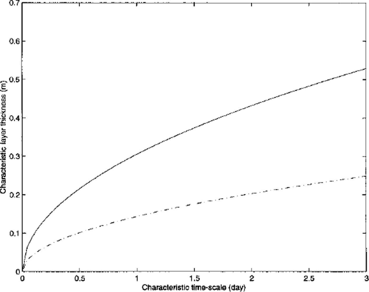
Fig. 1. Relationship between characteristic layer thickness and time-scale for two cases, representing the mid-winter multi-year ice condition (solid line) and the freeing first-year ice condition (dashed line) using equations (13) and (14). the two conditions were given by setting t = −30°c and s = 3.2 _ppt and t = −5.0˚c and s = 8.0 ppt, respectively.

The other observation is that we can roughly estimate a degree of sensitivity of each term appearing in Equation (4) by differentiating with respect to t_s{. This gives a first-order approximation for the sensitivity of the surface energy balance to the surface temperature, , ρ_aCpC_sua and 2ki/h, arising from the outgoing longwave radiation, sensible- and internal conductive-heat fluxes, respectively. It was found that this quantity, , is quasi-linear in the range that we are interested in. More importantly it is limited above by the freezing temperature (equal to fresh water) of the sea-ice surface, approximately 4.6 W m⁻² K−¹ at 0°C.

On the other hand, the other two terms vary with the wind speed and layer thickness. Substituting the numerical values of c_s = 1.75 × 10−³, p. =13 kg m−³, c_p = 1005 J kg"¹ K−¹ and ki = 2.034 Wm−¹K−¹ (see M78) the sensitivity of the last two terms is evaluated as 2.28w_a and 4/h, respectively. In other words, a case involving wind speeds of > 2 m s"¹ and/or layer thickness of < 0.8 m results in a high-sensitivity regime for the last two terms relative to the first term arising from the outgoing longwave radiation. In the context of our discussion, both terms become increasingly important with high-frequency variation in the forcing field, as the wind speed is likely higher and the layer thickness must be thinner as described above. Since the uppermost layer temperature 7\ and the surface temperature T_sf share the same sensitivity in the last term as 4/h, an accurate representation of the near-surface temperature gradient becomes equally important. For example, substituting h_eq = 30 cm corresponding to an e-folding time (τ_e) of 1 day into the relationship 4/h implies that in order to achieve the accuracy of 0(1 W m−²) for the conductive heat-flux term the uppermost layer temperature must be calculated within 0.075°C from a true temperature. In essence, this analysis demonstrates that the surface temperature and its gradient at the surface must be calculated with higher accuracy when high-frequency forcing variation is applied to a model.

Model Descriptions

The above analysis highlights two areas of importance in a model formulation when high-frequency variation in the forcing field is present: the choice of layer thickness, and calculation of the surface temperature and its gradient near the surface.

Layer structure

In previous models, the number of ice layers was fixed, making individual layer thickness dependent upon total ice thickness. In order to allow the models to obey thermal relaxation and to properly simulate the thermal inertia of the ice, these models used relatively thin layers. For example, a layer thickness of 10 cm was used in MU71, and 10 layers were used in EC93. Defining many layers carries a relatively high computational burden, and in climate models, where computational efficiency in each gridcell is critical, the burden can be large. This is particularly true in regions such as the Antarctic where seasonal sea ice is often very thin (and so many layers introduce an unnecessary restriction). We resolve this problem of matching layer thickness to forcing time-scale, by fixing the maximum layer thickness and changing the number of layers according to thinning and thickening of ice so as to avoid the burden of more ice layers than required to satisfy the thermal equilibrium condition.

Figure 2 presents a schematic of how the layer structure changes according to a change in total thickness. In this example, we set 30 cm as the maximum layer thickness. The method consists of two steps after the amount of growth and melt is determined at both the surface and the base. First the new number of layers and layer thickness according to a prescribed maximum layer thickness are calculated. Then a new temperature profile according to this new layer structure is determined. As is seen in Figure 2, the minimum thickness varies with total ice thickness. The total number of new layers is calculated as the integer part of the quotient of (total ice thickness/maximum layer thickness) plus one, except in a case consisting of a single layer. For example, if the total ice thickness and the maximum layer thickness were 200 and 30 cm, seven layers each 28.6 cm thick represent the ice column (see dashed line in Fig. 2). Conversely, when there are seven layers, a layer thickness can vary from 25.7 to 30 cm depending upon the total thickness. In the second step, we use the fact that the relationship between a profile based on mid-layer temperatures and another profile based on isothermal layer temperatures (thus the enthalpy-based profile) is described by a tn-diagonal linear system assuming the piece-wise linear temperature profile and constant heat capacity for each layer. When the number of layers is unchanged even with the presence of growth or melt, solving this linear system forward and backward gives the new temperature profile for the new layer structure that is determined in the first step. This scheme further preserves the original enthalpy of the total ice and snow, as well as the general vertical thermal gradients through the snow and ice. We execute this process at the end of each time-step. A linear structure given by this tridiagonal system makes this otherwise cumbersome relayering process fast and efficient.

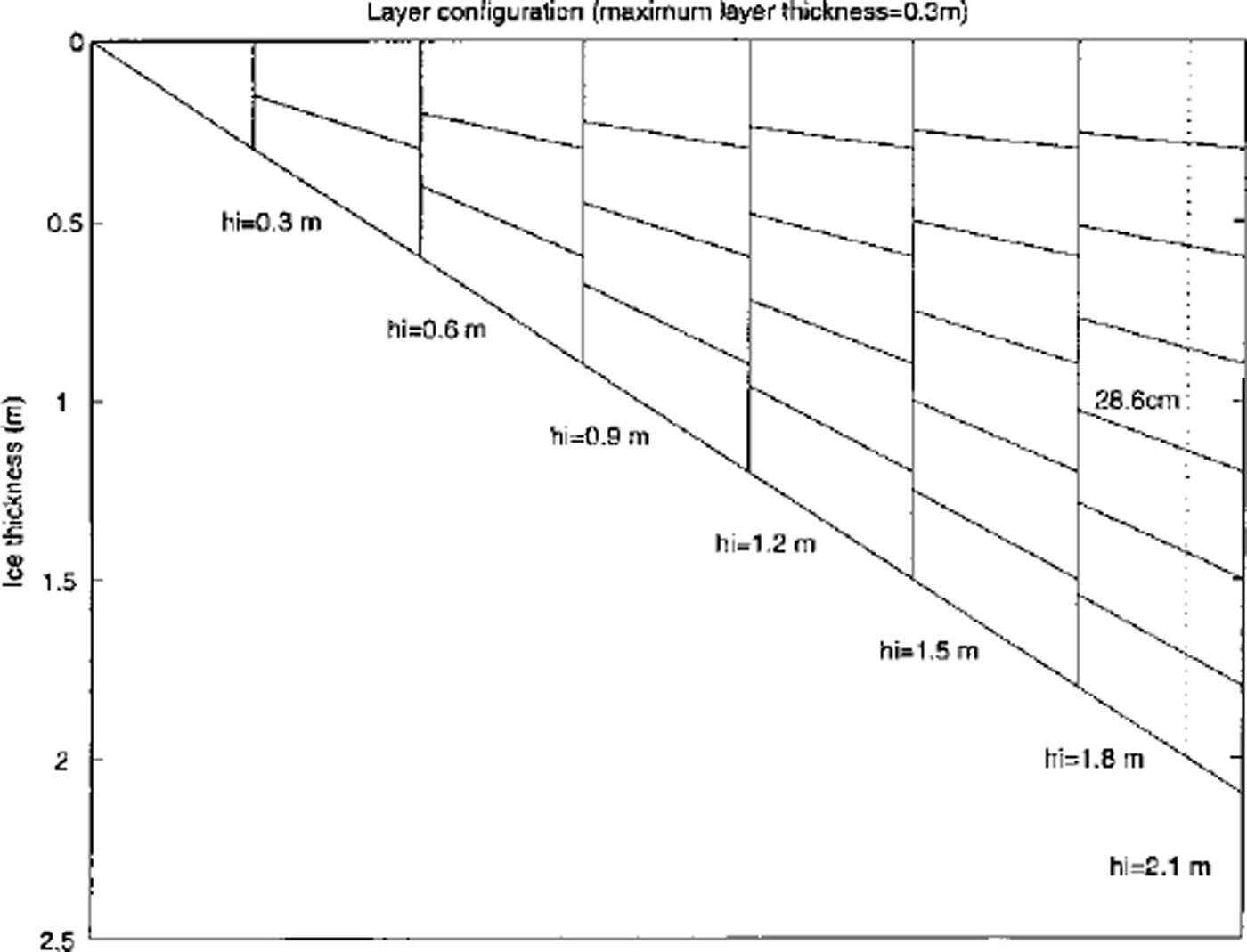
Fig. 2. Schematic for a varying layer structure with the maximum layer thickness set at 0.3 m for total thickness u_p to 2.1m. at each 0.3 m, another layer is added while smoothly varying the total thickness. the dotted line corresponds to a case with seven layers of 28.6 cm thickness, an example given in the text.

Temperature profiles

The previous analysis (above) also points out the necessity of calculating the surface temperature to a high degree of accuracy when high-frequency forcing is present. A standard scheme, introduced by MU71, solves Equation (4) with respect to the surface temperature t_s{ for a given value of the topmost layer temperature such as the value of 1\ from the previous time-step, T_1,0. This is done with an iterative procedure such as the Newton-Raphson method. A standard explicit or implicit scheme then uses this value to solve the heat equation (as long as the surface temperature is cooler than the melting point). This procedure, in which the surface flux boundary condition is decoupled from the rest of the system, could be accurate enough when the forcing changes slowly and smoothly.

However, when the forcing condition changes rapidly, so does the surface temperature. The variation in surface temperature associated with any changes in the forcing (per time-step) then introduces an error at each time-step, leading to a potential long-term bias. The above estimate of the desired level of accuracy for the uppermost layer temperature (i.e. 0.075°C required for the accuracy of 1 W m−² ) demonstrates the high sensitivity. At worst, this sensitivity does depend on the characteristic forcing timescale: the more variable the forcing the thinner the required maximum layer thickness. To minimize this source of error, which can be prohibitively large due to thin layer thickness required from short forcing time-scales, we employ an implicit numerical scheme as described below that also includes the surface temperature calculation as part of the conservation equation system.

To this end, the outgoing longwave radiation term in Equation (4) must be linearized with respect to some reference temperature. The topmost layer temperature from the previous time-step t_1, can be used as this reference temperature. An expansion of t_s{ with respect to t1, ₀ gives (to first order)

(7)

Then substituting Equation (7) into Equation (4) yields

(8a)

Further rearranging it gives

(8b)

which has the form required for inclusion into the linear system. Although this linearization introduces some error, it can be shown (and we have found) that a particular choice of the reference temperature has a negligible effect on the overall accuracy since is nearly linear over the relevant temperature range. Furthermore, as the analysis in the previous section shows, the error arising from this linearization is not only limited above, but also becomes smaller as the time-step becomes shorter (i.e. the shorter the time-step the smaller the change in temperature profile per time-step for a given change in the forcing), which allows an effective control on its influence if necessary.

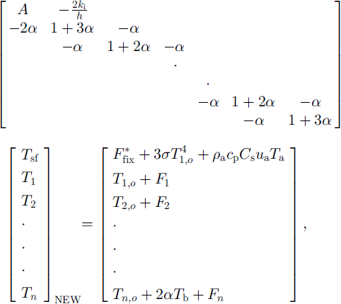
For the simplified case involving only ice layers (i.e. ignoring snow) the entire system is written as

(9)

where

(10)

(11)

δ_t is the time-step, and the vector [T _1,0 ,t _2,0 , . . . , …, t_n,0 ] and T_b denote a temperature profile from the previous step and the basal temperature fixed at the freezing point of the sea water, respectively. This is a tn-diagonal system, for which efficient algorithms are available, and it satisfies both internal and surface flux conditions simultaneously up to a prescribed degree of accuracy (at which they are provided).

In the above analysis some processes have been intentionally left out for illustrative purposes. For example, the latent-heat flux was held constant and parameterized as part of F_fix. It can be formulated through bulk formulation in much the same way as the sensible-heat flux. This is accomplished by applying the same procedure given in Equations (7) and (8) to a polynomial representation given in Equation (8) of M78 noting that there is a relationship between saturation vapor pressure and temperature. The penetration and absorption of shortwave radiation into the ice interior are known to influence the conduction of heat by introducing an internal heat source (Reference UntersteinerUntersteiner, 1964; MU71; Reference Grenfell and MaykutGrenfell and Maykut, 1977). These processes can also be incorporated into the present formulation by distributing part of F_fix to each layer. Let us denote shortwave radiation absorbed into each layer by f_i for i = 1, …, n. Then the presence of this internal heating source modifies Equation (9) as

(12)

where replaces F_fix, accounting for an adjustment of an amount of solar radiation penetrating into the interior.

Because of the presence of brine pockets that are trapped inside sea ice, the bulk thermal constants such as conductivity and heat capacity depend on both temperature and salinity Following the approximation made by Reference UntersteinerUntersteiner (1961), this dependence is commonly parameterized as

(13)

(14)

with the numerical values of k_i,k = 2.034 W m⁻¹ K−¹, (ρc)i, k = 1.883 × 106 J m–₃ KT¹, /3 = 04172 W m⁻¹ ppt−¹, ⁷ = 1.715 × 10⁷ J Km −3ppt−¹ , and some prescribed restrictions on s and t (see MU71). In the present formulation these functions evaluated at the temperature from the previous time-step are substituted into the linear system. This is equivalent to assuming that these thermal properties are constant within each layer and that a temperature profile does not change too much in a single time-step, an approach often adopted by other models (e.g. MU71, EC93; see Reference Bitz and LipscombBitz and Lipscomb, 1999, for an alternative approach). There are two sources of error associated with this approximation: one from assuming constant coefficient values for each layer, and the other from using old (from the previous step) temperatures to evaluate them. The former is related to the layer thickness and can be controlled by choosing thinner layers, giving an additional constraint to the maximum layer thickness. This becomes particularly important toward the base of the ice column and/or in the melting season when the ratio of ki/(ρc)i becomes smaller. The latter is a function of the time-step (the shorter the time-step the smaller the change in temperature), and so can be controlled by choosing a shorter time-step. Further, the error arising from this latter source can be limited by an iterative procedure, i.e. iterating with updated thermal coefficients with new temperatures (see Reference Bitz and LipscombBitz and Lipscomb, 1999, for their formulation). Given these identifications of the error sources and their relations to the layer thickness and time-step and the availability of the iterative procedure, all of which are discussed above, we adopt a simple method based on the temperature from the previous time-step as our base model structure.

Finally, the above formulation can be extended to include a snow cover. Assuming the basic case given Equation (9), the entire system is now expressed as

(15)

where

(16)

(17)

(18)

(19)

(20)

(21)

(22)

(23)

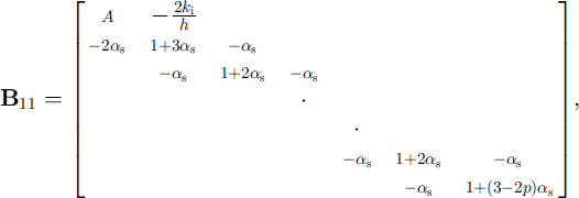
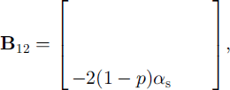
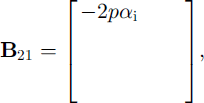
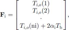
where T_s,₀(j) is the jth-layer snow temperature from the previous time-step for j = 1 , . . . , ns, t_{t 0}(j) is the jth-layer ice temperature from the previous time-step for j = 1 , . . . , ni , ns and ni are the numbers of layers for snow and ice, and h_s and hi are their layer thickness, a_s and a, are the coefficients (Equation(II)) evaluated for snow and ice, and p = (k_s/h_s)/ (k_s/h_s + ki/hi). Again all of the parameterizations for the latent-heat flux, the penetration of solar radiation, and the non-linear thermal coefficients can be implemented in the same manner as discussed above.

Control-Run Tests

Following the formulation described above, we have developed a thermodynamic sea-ice-snow model. Although our model still lacks parameterizations for a number of processes, such as spectral albedo and cloud effects on the solar penetration, lead formation and the stability effects on the turbulent fluxes, it does provide a solid foundation to which more physics can be added. The present formulation has sufficient details that allow basic control runs, with which the results can be compared with previous model studies using the same reference forcing as MU71 who studied the thermodynamic growth and melt, and their annual cycle of slab ice in the central Arctic (e.g. Reference SemtnerSemtner, 1976; Reference Parkinson and WashingtonParkinson and Washington, 1979; EC93). In order to facilitate comparison, we also used similar forcing data in our control runs, which consist of prescribed surface albedo, downward short- and longwave radiation, sensible- and latent-heat fluxes, the constant oceanic heat flux of 2 W m⁻², and 17% and 1.5 m⁻¹ as the fraction for the solar penetration and the extinction coefficient. We also assumed the longwave emissivity to be unity and the salinity in Equations (13) and (14) to be held at 3.2 ppt (see Table 1 for comparison of the prescribed annual total energy balances, and Figure 3a-c for the annual cycle of the snow depth, and both total and net longwave and shortwave radiation, respectively). For snow precipitation, we used semimonthly (in the fall) and monthly (in other seasons) values in a step-wise manner rather than a smoothly changing snow depth (e.g 1 January collects all snow for January and so on; values were taken from Reference Parkinson and WashingtonParkinson and Washington, 1979). The reason for this incremental approach was that it provides an excellent opportunity for testing our re-layering algorithm.

Table 1. Comparisons of key quantities in energy and mass balance between our model and mu and ec models

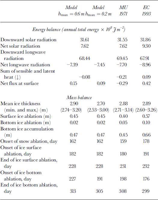
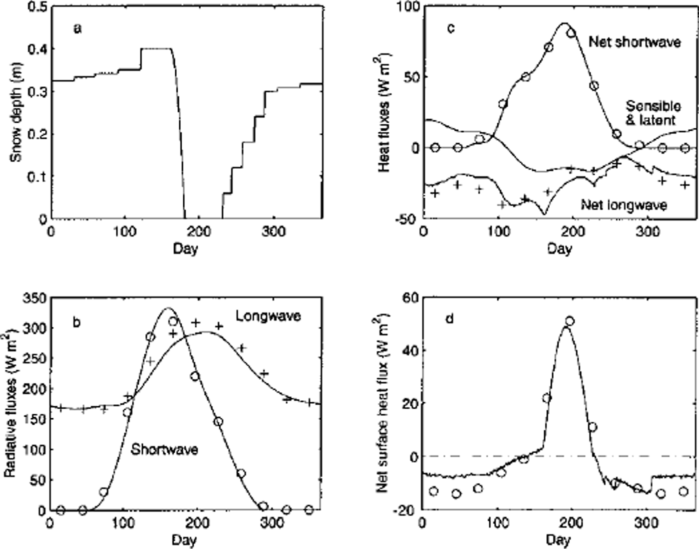
Fig. 3. Results from the control run. (a) the annual cycle of snow depth from the control run. note that it increases in an incremental manner (given) but decreases continuously (model calculated), ( b) the prescribed forcing of long- and shortwave radiation. plus and circle symbols indicate the monthly-averaged values used in mu71. (c) the prescribed net shortwave radiation (as albedo is prescribed in this control run) and the sum of the sensible- and latent-heat fluxes, and the calculated net longwave radiation. for comparison, circle (net shortwave) and plus (net longwave) indicate the values used in mu71. ( d) the net heat surface flux and circles from mu71.

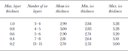
We used 2.7 m of ice with a linear temperature profile as our initial condition. By taking advantage of our implicit scheme we run the model with a time-step of 24 h. After 20−30 years of integration depending on a vertical resolution, the equilibrium annual cycle was reached. Figure 4 shows the equilibrium annual cycle and the time series of annual mean, minimum and maximum thickness over the integration period for the case with the maximum snow and ice thickness of 0.3 and 0.6 m, respectively. Table 1 summarizes the energy and mass balance of the equilibrium annual cycles from the control run and its counterpart in MU 71 and EC93. With the maximum ice-layer thickness set at 0.6 m, equivalent to 5−6 layers, our model predicts a similar equilibrium annual cycle to that of the MU model (i.e. within ±6 cm for the mean, minimum and maximum ice thickness). With this resolution the monthly mean thickness is in close agreement with that of MU71 (shown in Fig. 4a as circles). As the vertical resolution of our model was increased to the maximum layer thickness of 0.2 m, equivalent to 13−15 layers, the mean equilibrium thickness dropped from 2.90 m to 2.70 m, with similar decreases found in both the minimum and maximum thickness. By contrast, the amount of surface and bottom ablation and bottom accumulation was relatively unchanged between two cases (i.e. the maximum difference was <1 cm). It varies across different models, however: for example, our model predicted a net bottom accumulation of 0.45 m, whereas the MU and EC models gave 0.4 and 0.56 m, respectively. These differences are due in large part to a varying degree of complexity in surface albedo parameterizations across the models (EC93), but also reflect differences that exist in the forcing conditions (i.e. Table 1 shows that the net heat flux at the surface varies considerably: −0.29 M J m⁻² in MU71 to 0.42 MJ m⁻² in EC93, and ours in between). It was found that the difference in the net heat flux at the surface between MU71 and our model had seasonal dependence as seen in Figure 3d. As the amount of net shortwave radiation is almost identical in both models (Fig. 3c), this difference in the net surface heat flux must be associated with the difference in the surface temperatures, perhaps an indication of the effect of different numerical schemes. Despite these differences, our model seems to simulate the equilibrium annual cycle in a reasonably close agreement with previous studies under similar forcing conditions.

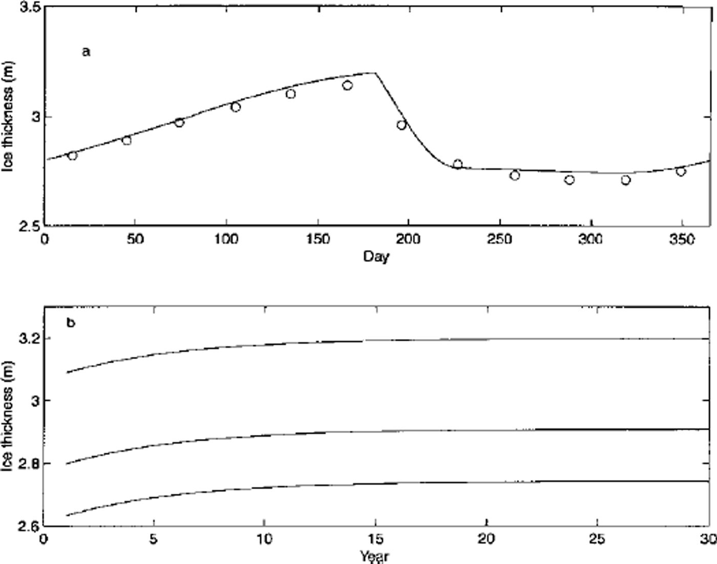
Fig. 4. Model output from a control run with a maximum layer thickness of 0.6 m (5−6 layers), (a) the equilibrium annual cycle of the 30th year. circles indicate the monthly mean values of mu71. (b) a time series of annual maximum, mean and minimum ice thickness in the first 30 years of run.

We also evaluated the effect of vertical resolution by changing the maximum layer thickness from 1.0 m to 0.2 m with an increment of 0.2 m, which is equivalent to changing the number of layers from 3 to 13 layers (see Table 2). The results show the variation in the equilibrium mean thickness, ranging from 2.70 m with a maximum layer thickness of 0.2 m, to 2.99 m with a maximum layer thickness of 1.0 m. This contrasts with the results of Reference SemtnerSemtner’s (1976) experiment, in which he found a converging yet increasing trend in the equilibrium thickness with an increasing number of layers.

Table 2. The equilibrium annual cycle with different vertical resolution

To examine the source of this difference we further examined the internal temperature profiles for both snow and ice (Fig. 5). The lefthand column shows a progression of the temperature profile showing both warming and melting of the snow layer and simultaneous ice accumulation during spring from day 105 to day 175. For example, the number of ice layers changed from five to six between day 105 (Fig. 5a) and day 135 (Fig. 5b). The righthand column marks a period of warming and thinning of ice, followed by snowfall in early autumn from day 182 to day 244, with a decrease in the number of layers from six to five between day 182 (Fig. 5e) and day 196 (Fig. 5f). Strongly visible is a thermal inertia effect that results in non-linear profiles throughout both periods. This curvature effect near the base is more accurately represented when the vertical resolution becomes finer (not shown here). As the rates of the basal ice accumulation/ ablation are directly related to the temperature gradient at the boundary, this affects the calculation of timing and duration of the bottom ablation (see Table 1).

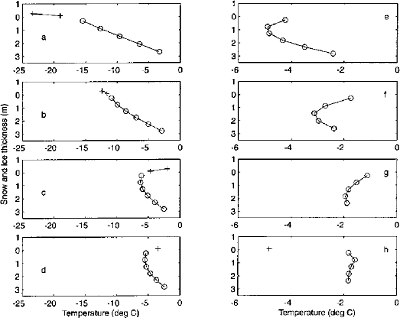
Fig. 5. A time series of temperature profiles for snow (plus) and ice (circle) at (a) day 105, (b) day 135, (c) day 165, (d) day 175, (e) day 182, (f) day 196, (g) day 230 and (h) day 244.

In particular, the timing of the bottom ablation has significant dependence on the vertical resolution. This seems to suggest that a combined effect, arising both from the differences in the parameterizations of the brine pockets and the absorption of the solar radiation between Semtner’s (using the heat reservoir) and our model (using temperature-dependent thermal properties) and from the differences in the surface temperature calculation, accounts for the different behavior found in the equilibrium ice thickness.

Conclusions

Analysis of the heat equation not only shows a need for refining model construction for sea ice and snow thermodynamics to better account for the thermal response to high-frequency forcing variability, but also identifies specific areas that need to be improved. These considerations led us to develop a new adjustable-layering thermodynamic model. In particular, we addressed two specific needs by (1) restructuring layers while conserving overall enthalpy and general temperature gradient, and (2) computing the temperature profile implicitly including the surface flux boundary condition (allowing a consistent simultaneous solution to the ice or snow surface temperature).

Overall, the model reproduces results similar to those of previous models under smooth forcing conditions, but because of our numerical formulation this adjustable-layering model is equally valid for high-frequency forcing variability. Additional refinement and tests are still necessary, but the general technique and implementation of the adjustable layering and simultaneous surface solution are demonstrated. The present model structure is efficient in the sense that it uses only the minimum number of layers required to satisfy the numeric approximation, which is ideal for climate models where the surface temperature of the ice or snow is critical for long-term stability in the climate. Our model achieves this at a cost of performing a matrix inversion three times during a single time-step, once for calculating the temperature profile and twice for the re-layering scheme. However, because of the tri-diagonal system that we solve each time, this procedure only takes o(n) operations (n being the number of layers), not to mention that n is optimally determined according to the forcing conditions. In addition, the inclusion of the surface flux boundary condition into the temperature calculation with an implicit scheme allows a longer time-step, which in fact can be used as a stand-alone module. Another issue regarding the layering structure is that there is no a priori reason for using the same layer thickness throughout the snow/ice column, and our model formulation can easily adopt variable-layer formulation by assigning different layer thickness to Equation (12) or (15). It is conceivable to optimally formulate a variable-layer-thickness structure in both a physical and a numerical sense. However, this requires a careful model experiment and comparisons with in-site measurements. Clearly there is a trade-off between the efficiency and the accuracy associated with the whole or part of the present formulation. We hope to explore the issue of computational efficiency and further test the model against the recent field experiment results (in the Arctic and Antarctic) where we can examine the fidelity with which the adjustable layers preserve the interior temperature profiles through the ice and snow. We also intend to add more physics to the model, accommodating melt-pond formation, surface albedo variability, etc. Some of the processes, such as melting and freezing of flooded snow, geometrical effects on lateral and basal melting using statistical description of floe size and shape, and frazil growth in a lead, have already been formulated. While these other characteristics, still under investigation, will be presented in a later companion paper, we focus here on the basic philosophy and numerics of the thermodynamics calculation, and specifically on the adjustable-layer scheme developed within.