Hostname: page-component-cd9895bd7-jn8rn Total loading time: 0 Render date: 2025-01-03T21:13:03.903Z Has data issue: false hasContentIssue false

Effect of random roughness on Stokes flow

Published online by Cambridge University Press:  25 November 2024
Gerardo Severino*
Affiliation:
Division of Water Resources Management, University of Naples - Federico II, via Universitá 100, Portici, I80055 NA, Italy
*
Email address for correspondence: [email protected]

Abstract

Microscopic irregularity (roughness) of bounding surfaces affects macroscopic dynamics of fluid flows. Its effect on bulk flow is usually quantified empirically by means of a roughness coefficient. A new approach, which treats rough surfaces (e.g. parallel plates) as random fields whose statistical properties can be inferred from measurements, is presented. The mapping of a random flow domain onto its deterministic counterpart, and the subsequent stochastic averaging of the transformed Stokes equations, yield expressions for the effective viscosity and roughness coefficient in terms of the statistical characteristics of the irregular geometry of the boundaries. The analytical nature of the solutions allows one to handle surface roughness characterized by short correlation lengths, a challenging feature for numerical stochastic simulations.

Type
JFM Rapids
Copyright
© The Author(s), 2024. Published by Cambridge University Press

1. Introduction

Microscopically irregular geometry of bounding walls affects a plethora of physical, biological and chemical phenomena. For example, rough surfaces of rock fractures impact both the extraction of natural resources and the subsurface migration of contaminants (e.g. Lenci et al. Reference Lenci, Méheust, Putti and Di Federico2022; Viswanathan et al. Reference Viswanathan2022). Irregular surfaces play an important role in the design of miniaturized electro-mechanical devices (e.g. Nawaz et al. Reference Nawaz, Masood, Saleem, Iqbal and Zubair2020; Navajas et al. Reference Navajas, Pérez-Escudero, Martínez-Hernández, Goicoechea and Liberal2023) and computer technologies (Murthy, Duwensee & Talke Reference Murthy, Duwensee and Talke2010; Li et al. Reference Li, Fu, Zhou, Sun, Li, Wu and Dai2022). Irregularity of a vessel's cross-section lined with endothelial tissue can greatly alter blood flow (Park, Intaglietta & Tartakovsky Reference Park, Intaglietta and Tartakovsky2012; Yi et al. Reference Yi, Tian, Simmons and Barber2022) and biochemistry (Hightower et al. Reference Hightower2011; Park, Intaglietta & Tartakovsky Reference Park, Intaglietta and Tartakovsky2015). Surface irregularity of coronary arteries is linked to the onset of atherosclerosis (Owen et al. Reference Owen, Schenkel, Shepherd and Espino2020; Yamane et al. Reference Yamane, Mori, Arakawa, Wilhjelm and Kanai2023), etc.

In these and other applications, the irregular geometry of bounding surfaces manifests itself at length scales ranging from nanometres (e.g. in electronic and biomedical devices) to millimetres (e.g. in geologic media). It is sometimes argued that in a channel of large aperture, i.e. when the relative height of the non-smooth surface does not exceed 5 % of aperture, the impact of surface roughness on laminar flow can be neglected (e.g. Moody Reference Moody1944; Webb & Kim Reference Webb and Kim1994). Yet, in many cases of practical significance (see the references above, among many others), the surface geometry is of paramount importance and correlation between the surface texture and the flow variables is well established (e.g. Brown Reference Brown1987, Reference Brown1989; Kandlikar et al. Reference Kandlikar, Schmitt, Carrano and Taylor2005). In particular, wall geometry directly affects the friction factor (Wang, Yap & Mujumdar Reference Wang, Yap and Mujumdar2005) and can increase the Poiseuille number by the factor of three relative to a smooth wall (Kandlikar et al. Reference Kandlikar, Schmitt, Carrano and Taylor2005, and references therein).

Challenges in fluid-flow simulations in the presence of boundaries with an irregular topology start with a proper representation of surface texture. One approach is to represent a solid surface by canonical geometrical forms, such as sinusoidal or sawtooth shapes (e.g. Plouraboué, Geoffroy & Prat Reference Plouraboué, Geoffroy and Prat2004; Tavakol et al. Reference Tavakol, Froehlicher, Holmes and Stone2017; Dewangan Reference Dewangan2024) or fractals (Chen et al. Reference Chen, Zhang, Shi and Peterson2009). Such representations work well in some settings, but are often too simplistic to mimic the disordered structures (Brown, Stockman & Reeves Reference Brown, Stockman and Reeves1995; Wang et al. Reference Wang, Yap and Mujumdar2005; Gamrat et al. Reference Gamrat, Favre-Marinet, Le Person, Baviere and Ayela2008; Herwig, Gloss & Wenterodt Reference Herwig, Gloss and Wenterodt2008; Maggiolo, Manes & Marion Reference Maggiolo, Manes and Marion2013; Severino et al. Reference Severino, Giannino, De Paola and Di Federico2023). An alternative approach is to treat a rough surface as a random field, whose statistics are either prescribed or inferred from observations (Bahrami, Yovanovich & Culham Reference Bahrami, Yovanovich and Culham2006a,Reference Bahrami, Yovanovich and Culhamb; Yamane et al. Reference Yamane, Mori, Arakawa, Wilhjelm and Kanai2023).

This approach, which we adopt in this study because of its generality, gives rise to a class of problems involving partial differential equations on random domains (Xiu & Tartakovsky Reference Xiu and Tartakovsky2006). Their numerical treatment typically involves a finite-term representation of random surfaces via, for example, truncated Karhunen–Loève (KL) expansions or Fourier series (Tartakovsky & Xiu Reference Tartakovsky and Xiu2006; Park et al. Reference Park, Intaglietta and Tartakovsky2012; Zayernouri et al. Reference Zayernouri, Park, Tartakovsky and Karniadakis2013; Kwon & Tartakovsky Reference Kwon and Tartakovsky2020; Zheng et al. Reference Zheng, Valdebenito, Beer and Nackenhorst2023). Since the convergence rate of KL expansions deteriorates as the correlation length of the underling random field decreases, such numerical solutions become computationally intractable when dealing with a surface exhibiting short correlation lengths if not white noise (zero correlation length).

While posing a computational challenge that is often referred to as ‘the curse of dimensionality’, short correlation lengths (accompanied by small standard deviations from a flat surface) are well suited for perturbation-based strategies of stochastic homogenization. We use this approach to derive analytical expressions for the effective viscosity and friction factor for Stokes flow between two parallel plates whose irregular geometry is treated within a stochastic framework that regards them as random fields. Section 2 contains a problem formulation. The solution method (§ 3) consists of two parts: a stochastic mapping of the random flow domain on its deterministic canonical counterpart (§ 3.1), and averaging of the transformed flow equations (§ 3.2). Results are discussed in § 4 followed by concluding remarks.

2. Problem formulation

We consider steady, isothermal and fully developed Stokes flow of an incompressible fluid with viscosity $\mu$ and density $\rho$. The flow takes place in an infinite horizontal channel $\mathcal {D}$ bounded at the top and bottom by rough (orange face in figure 1) impermeable surfaces $z_{top} \equiv z_{top}(\boldsymbol {x}_r)$ and $z_{bot} \equiv z_{bot}(\boldsymbol {x}_r)$, i.e. $\mathcal {D} = \{ \boldsymbol {x} \equiv (x_1, x_2, x_3): \boldsymbol {x}_r \equiv (x_1, x_2) \in \mathbb {R}^2, \; z_{bot} \le x_3 \le z_{top}\}$. The flow is driven by an externally imposed pressure gradient $\partial p / \partial x_1$ in the $x_1$ direction. Fluid velocity $\boldsymbol {v}(\boldsymbol {x}) = (v_1, v_2, v_3)^\top$ and pressure $p(\boldsymbol {x})$ satisfy momentum and continuity equations

(2.1)\begin{equation} \left.\begin{array}{c@{}} \mu \nabla^2 \boldsymbol{v} = \boldsymbol{\nabla} p, \\ \boldsymbol{\nabla} \boldsymbol{\cdot} \boldsymbol{v} = 0, \end{array}\right\}\quad \boldsymbol{x} \in \mathcal{D}, \end{equation}

respectively. If the channel walls were smooth, the aperture would be constant $b$, and (2.1) would give rise to the parabolic velocity profile (Hagen–Poiseuille law). Instead, the upper and lower surfaces exhibit microscopic spatial fluctuations (figure 1), which are modelled as random fields, i.e. $z_{top} \equiv z_{top}(\boldsymbol {x}_r;\omega )$ and $z_{bot}\equiv z_{bot}(\boldsymbol {x}_r;\omega )$, where $\omega$ is a realization from the sample space.

Figure 1. Frontal (i) and longitudinal (ii) views of two parallel plates (aperture $b$) hosting the flow. The domain is such that $( x_1, x_2 ) \in \mathbb {R}^2$, whereas the vertical coordinate $x_3 \in [z_{bot}, z_{top}]$ is bounded between the top and bottom irregular surfaces (orange face).

The top $z_{top}(\boldsymbol {x}_r;\omega )$ and the bottom $z_{bot}(\boldsymbol {x}_r;\omega )$ are assumed to be mutually independent second-order stationary random fields with, in particular, standard deviations, $\sigma _{z_{bot}}$ and $\sigma _{z_{top}}$. In keeping with the physical meaning of wall roughness, we take $\sigma _{z_{bot}},\sigma _{z_{top}} \ll b$, so that the two surfaces do not overlap at any point $\boldsymbol {x}_r$ with probability $\mathbb {P} = 1$. Since $\mathbb {P} \{ z_{top} - z_{bot} > 0 \} = 1$ and $\mathbb {P} \{ z_{top} > 0 \} = 1$, we treat the random fields $Y(\boldsymbol {x}_r; \omega ) = - \ln ( z_{top} - z_{bot} )$ and $\zeta (\boldsymbol {x}_r; \omega ) = - \ln z_{top}$ as multivariate Gaussian. Finally, both $z_{top}(\boldsymbol {x}_r;\omega )$ and $z_{bot}(\boldsymbol {x}_r;\omega )$ are assumed to be mean-square differentiable with respect to $x_i$ ($i=1,2$) on their domains of definition (Yaglom Reference Yaglom1987). The accuracy and robustness of such an assumption (that has been adopted in other works on similar topics, see e.g. Tartakovsky & Xiu Reference Tartakovsky and Xiu2006; Zayernouri et al. Reference Zayernouri, Park, Tartakovsky and Karniadakis2013) have been assessed by Wang et al. (Reference Wang, Yap and Mujumdar2005). However, it is worth noting that the present study allows also dealing with other models (not necessarily Gaussian) for the random fields $Y$ and $\zeta$.

We recast the problem in a dimensionless form by rescaling the coordinates and flow variables,

(2.2ae)\begin{equation} \hat{\boldsymbol{x}} = \frac{\boldsymbol{x}}{b}, \quad \hat{\boldsymbol{v}} = \frac{\mu \boldsymbol{v}}{\rho g b^2}, \quad \hat h = \frac{p}{\rho g b}, \quad \hat{z}_{top} = \frac{z_{top}}{b}, \quad \hat{z}_{bot} = \frac{z_{bot}}{b}, \end{equation}

where $g$ is the gravitational acceleration constant. Then, (2.1) is replaced with

(2.3)\begin{equation} \left.\begin{array}{c@{}} \hat{\nabla}^2 \hat{\boldsymbol{v}} = \hat{\boldsymbol{\nabla}} \hat h, \\ \hat{\boldsymbol{\nabla}} \boldsymbol{\cdot} \hat{\boldsymbol{v}} = 0, \end{array}\right\}\quad \hat{\boldsymbol{x}} \in \hat{\mathcal{D}}(\omega). \end{equation}

Randomness of $\hat {\mathcal {D}}$ renders $\hat {\boldsymbol {v}} \equiv ( \hat {v}^1, \hat {v}^2, \hat {v}^3 )^\top$ and $\hat {\boldsymbol {\nabla }} \hat h$ random, as well. In what follows, we drop the hats $\hat {\cdot }$ to simplify the notation. Our goal is to derive an ensemble-averaged solution to this problem.

3. Stochastic averaging of flow problem

Monte Carlo simulations, a go-to technique used to solve problems with random coefficients, are ill-suited for solving (2.3). That is because each random realization of the flow domain $\mathcal {D} (\omega )$ requires a fine (and non-uniform) mesh to resolve small-scale geometry of the surface, and the between-realizations variability of the nodes in such meshes complicates the sample averaging of model outputs. Instead, we pursue a two-stage strategy detailed below.

3.1. Random domain mapping

We use the change of coordinates

(3.1a,b)\begin{equation} \xi^i = x_i \quad (i =1,2), \quad \xi^3=\frac{x_3 - z_{bot} }{z_{top} - z_{bot}}, \end{equation}

to map the random domain $\mathcal {D}$ onto a deterministic domain $\mathcal {A} =\{\boldsymbol {\xi } \equiv (\xi ^1, \xi ^2, \xi ^3)^\top : (\xi ^1, \xi ^2) \in \mathbb {R}^2, \ 0\le \xi ^3\le 1 \}$. A general mapping $\boldsymbol {x} \mapsto \boldsymbol {\xi }$ transforms the differential operators in (2.3), i.e. the gradient, the Laplacian and the divergence, according to Arfken & Weber (Reference Arfken and Weber2005):

(3.2ac)\begin{equation} \frac{\partial}{\partial x_i} \mapsto g^{ik}\dfrac{\partial}{\partial \xi^k}, \quad \nabla^2 \mapsto \frac{1}{ \sqrt { |\tilde g| } } \frac{\partial}{\partial \xi^j} \left( \sqrt{ |\tilde g| } g^{jk} \frac{\partial}{\partial \xi^k} \right), \quad \boldsymbol{\nabla} \boldsymbol{\cdot} \boldsymbol{v} \mapsto \frac{1}{ \sqrt{ |\tilde g| } } \frac{\partial}{\partial \xi^k} ( \sqrt{ |\tilde g| } v^k ). \end{equation}

Here and below the Einstein notation is used to indicate the summation over repeated indices, $\tilde g$ is the determinant of the covariant metric tensor $\boldsymbol {g}$ with components $g_{i k} = \boldsymbol {\varepsilon }_i \boldsymbol {\cdot } \boldsymbol {\varepsilon }_k$, where $\boldsymbol {\varepsilon }_i \equiv \partial \boldsymbol {x} / \partial \xi ^i$. Components $g^{ik}$ of the contravariant metric tensor are related to their covariant counterparts $g_{ik}$ via the transformation $g^{ik} = \mathcal {C}( g_{ik}) / |\tilde g|$, where $\mathcal {C} ({\cdot })$ is the operator of tensorial conjugation. This general mapping, $\boldsymbol {x} \mapsto \boldsymbol {\xi }$, transforms flow equations (2.3) into

(3.3)\begin{equation} \left.\begin{array}{c@{}} \dfrac{\partial}{\partial \xi^j} \left( \mathcal{G}^{jk} \dfrac{\partial v^i}{\partial \xi^k} \right) = \mathcal{G}^{ik} \dfrac{\partial h}{\partial \xi^k},\\ \dfrac{\partial}{\partial \xi^k} ( v^k |\tilde g|^{1/2} ) = 0, \end{array}\right\} \end{equation}

with $\mathcal {G}^{ij} = |\tilde g|^{1/2} g^{ij}$.

For the particular mapping $\boldsymbol {x} \mapsto \boldsymbol {\xi }$ in (3.1), these general expressions become (where $\boldsymbol{e}_i$ are the unit vectors)

(3.4a)\begin{gather} \boldsymbol{\varepsilon}_i = \frac{\partial}{\partial \xi^i} \{ \xi^1 \boldsymbol{e}_1 + \xi^2 \boldsymbol{e}_2 + [ \xi^3 (z_{top} - z_{bot} ) + z_{bot} ] \boldsymbol{e}_3 \}, \end{gather}
(3.4b) \begin{gather}{}[ g_{ij}] = \left[\begin{array}{ccc} 1+\alpha^2_1 & \alpha_1 \alpha_2 & \alpha_1 ( z_{top} - z_{bot} ) \\ \alpha_1 \alpha_2 & 1+\alpha^2_2 & \alpha_2 ( z_{top} - z_{bot} )\\ \alpha_1 ( z_{top} - z_{bot} ) & \alpha_2 ( z_{top} - z_{bot} ) & ( z_{top} - z_{bot} )^2 \end{array}\right], \end{gather}
(3.4c)\begin{gather}\alpha_m = \xi^3 \frac{\partial}{\partial \xi^m} ( z_{top} - z_{bot} ) + \frac{\partial z_{bot}}{\partial \xi^m}, \quad m=1,2. \end{gather}

The determinant of this $[g_{ij}]$ is $\tilde g = ( z_{top} - z_{bot} )^2$, which gives rise to the contravariant tensor

(3.4d) \begin{equation} [g^{ij} ] \equiv \left[\begin{array}{ccc} 1 & 0 & -\dfrac{\alpha_1}{z_{top} - z_{bot}} \\ 0 & 1 & -\dfrac{\alpha_2}{z_{top} - z_{bot} } \\ -\dfrac{\alpha_1}{z_{top} - z_{bot}} & - \dfrac{\alpha_2}{z_{top} - z_{bot}} & \dfrac{1 + \alpha^2_1 + \alpha^2_2}{( z_{top} - z_{bot} )^2} \end{array}\right]\end{equation}

and

(3.4e) \begin{equation} [\mathcal{G}^{ij} ] = \left[\begin{array}{ccc} z_{top} - z_{bot} & 0 & -\alpha_1 \\ 0 & z_{top} - z_{bot} & -\alpha_2 \\ -\alpha_1 & - \alpha_2 & \dfrac{1 + \alpha^2_1 + \alpha^2_2}{z_{top} - z_{bot}} \end{array}\right]. \end{equation}

With these results, flow equations (3.3) transform into

(3.5) \begin{equation} \left.\begin{array}{c@{}} \mathcal{G}^{jk} \dfrac{\partial^2 v^i}{\partial \xi^j \partial \xi^k} + \dfrac{\partial \mathcal{G}^{jk}}{\partial \xi^j} \dfrac{\partial v^i}{\partial \xi^k} = \mathcal{G}^{ik} \dfrac{\partial h}{\partial \xi^k}, \\ v^k \dfrac{\partial}{\partial \xi^k} ( z_{top} - z_{bot} ) + ( z_{top} - z_{bot}) \dfrac{\partial v^k}{\partial \xi^k} = 0, \end{array}\right\}\quad \boldsymbol{\xi} \in \mathcal{A}. \end{equation}

This procedure transforms deterministic partial differential equations (PDEs) on the random domain $\mathcal {D}$ into PDEs with random coefficients on the deterministic domain $\mathcal {A}$, with the computational advantage of allowing to disregard the impact of the rough topology of the domain $\mathcal {D}$. If the walls were smooth, then $z_{top} - z_{bot} \equiv 1$ and $\mathcal {G}^{ij} \equiv \delta ^i_j$, so that (3.5) would coincide with (2.3).

3.2. Stochastic averaging

In (3.5), the surface roughness is represented by two log-normal random fields, $z_{top} - z_{bot} = \exp ( -Y )$ and $z_{top} = \exp ( - \zeta )$. Since $\sigma _Y$ and $\sigma _\zeta$, the standard deviations of $Y(\boldsymbol {x}_r;\omega )$ and $\zeta (\boldsymbol {x}_r;\omega )$, are small, we expand the model inputs and outputs into asymptotic series (e.g. Severino & De Bartolo Reference Severino and De Bartolo2015, and references therein):

(3.6) \begin{equation} \left.\begin{array}{c@{}} \displaystyle z_{top} - z_{bot} = \sum_n \dfrac{({-}Y)^n}{n!}, \quad z_{top} = \sum_n \dfrac{(-\zeta)^n}{n!}, \\ \displaystyle \boldsymbol{v} = \sum_n \boldsymbol{v}_{(n)}, \quad h = \sum_n h_{(n)}, \quad \mathcal{G}^{ij} = \sum_n \mathcal{G}^{ij}_{(n)}, \end{array}\right\} \end{equation}

where the subscript $_{(n)}$ denotes terms of order $O (\gamma ^n)$, for $\gamma \equiv Y, \zeta$. Substituting (3.6) into (3.5) and collecting the terms of equal orders yields a recursive set of boundary-value problems (BVPs),

(3.7a) \begin{equation} \left.\begin{array}{c@{}} \nabla^2 v^i_{(n)} - \dfrac{\partial}{\partial \xi^i} h_{(n)} = \mathcal{F}^i_{(n)} \\ \boldsymbol{\nabla} \boldsymbol{\cdot} \boldsymbol{v}_{(n)} = \mathcal{Q}_{(n)} \end{array}\right\}\quad n = 0, 1, 2, \end{equation}

with $\mathcal {F}^i_{(0)} = \mathcal {Q}_{(0)} \equiv 0$;

(3.7b)\begin{equation} \mathcal{F}_{(1)}^i \equiv \mathcal{G}^{ik}_{(1)} \dfrac{\partial h_{(0)}}{\partial \xi^k} - \dfrac{\partial}{\partial \xi^j} \left[ \mathcal{G}^{jk}_{(1)} \dfrac{\partial v^i_{(0)}}{\partial \xi^k} \right], \quad \mathcal{Q}_{(1)} \equiv \boldsymbol{v}_{(0)} \boldsymbol{\cdot} \boldsymbol{\nabla} Y \end{equation}

and

(3.7c) \begin{equation} \left.\begin{array}{c@{}} \mathcal{F}_{(2)}^i \equiv \mathcal{G}^{ik}_{(2)} \dfrac{\partial h_{(0)}}{\partial \xi^k} + \mathcal{G}^{ik}_{(1)} \dfrac{\partial h_{(1)}}{\partial \xi^k} - \dfrac{\partial}{\partial \xi^j} \left[ \mathcal{G}^{jk}_{(2)} \dfrac{\partial v^i_{(0)}}{\partial \xi^k} + \mathcal{G}^{jk}_{(1)} \dfrac{\partial v^i_{(1)}}{\partial \xi^k} \right], \\ \mathcal{Q}_{(2)} \equiv \boldsymbol{\nabla} \boldsymbol{\cdot} [ Y \boldsymbol{v}_{(1)} ] - \dfrac{\boldsymbol{v}_{(0)}}{2} \boldsymbol{\cdot} \boldsymbol{\nabla} Y^2. \end{array}\right\} \end{equation}

The algebraic manipulations leading to these expressions account for the divergent-free condition, $\boldsymbol {\nabla } \boldsymbol {\cdot } \boldsymbol {v}_{(0)} = 0$, satisfied by the leading-order approximation of the velocity field $\boldsymbol {v}(\boldsymbol {\xi })$. The first-order term in the expansion of tensor $\boldsymbol {\mathcal {G}}$ in (3.4e) is

(3.8) \begin{equation} [\mathcal{G}^{ij}_{(1)} ] = \left[\begin{array}{ccc} -Y & 0 & \dfrac{\partial \zeta}{\partial \xi^1} - ( 1 - \xi^3 ) \dfrac{\partial Y}{\partial \xi^1} \\ 0 & -Y & \dfrac{\partial \zeta}{\partial \xi^2} - ( 1 - \xi^3 ) \dfrac{\partial Y}{\partial \xi^2} \\ \dfrac{\partial \zeta}{\partial \xi^1} - ( 1 - \xi^3 ) \dfrac{\partial Y}{\partial \xi^1} & \dfrac{\partial \zeta}{\partial \xi^2} - ( 1 - \xi^3 ) \dfrac{\partial Y}{\partial \xi^2} & Y \end{array}\right], \end{equation}

and the ensemble mean of the second-order term is $\mathbb {E} \{ \mathcal {G}^{ij}_{(2)} \} = \delta ^i_j \sigma ^2_Y / 2$.

The leading-order BVP in (3.7) is deterministic, corresponding to the classical problem of Stokes flow between smooth parallel plates. Its solution is the Hagen–Poiseuille law,

(3.9ac)\begin{equation} v^1_{(0)} ( \xi^3 ) = \frac{\mathcal{J}}{2} ( 1 - \xi^3 ) \xi^3, \quad v^2_{(0)} = v^3_{(0)} \equiv 0, \quad \frac{{\rm d} h_{(0)}}{{\rm d} \xi^1} = \mathcal{J}. \end{equation}

The first-order correction is $\mathbb {E} \{\boldsymbol {v}_{(1)}(\boldsymbol {\xi }) \} = 0$ and $\mathbb {E} \{ h_{(1)}(\boldsymbol {\xi }) \} = 0$. By limiting the analysis to the case of a signal $w$ characterized by a long range of correlation, the second-order correction satisfies the deterministic BVP (Appendix A)

(3.10) \begin{equation} \left.\begin{array}{c@{}} \nabla^2 \bar v^i_{(2)} ={-} \mathcal{J} \sigma^2_Y \delta^i_1, \\ \boldsymbol{\nabla} \boldsymbol{\cdot} \bar{\boldsymbol{v}}_{(2)} = 0, \end{array}\right\} \end{equation}

where $\mathbb {E}\{A\} \equiv \bar A$ for any random variable $A$.

4. Discussion and concluding remarks

We now aim at deriving Stokes equations satisfied by mean velocity $\bar {\boldsymbol {v}} = \boldsymbol {v}_{(0)} + \bar {\boldsymbol {v}}_{(2)}$ and mean pressure head $\bar h = h_{(0)} + \bar {h}_{(2)}$. This is achieved by summing up (3.7) and taking the expectation after replacing $\bar {\mathcal {F}}_{(2)}^i \mapsto - \mathcal {J} \sigma ^2_Y \delta ^i_1$ to have

(4.1) \begin{equation} \left.\begin{array}{c@{}} \nabla^2 \bar{v}^{\,i} - \dfrac{\partial \bar h}{\partial \xi^i} ={-} \mathcal{J} \sigma^2_Y \delta^i_1 \\ \dfrac{\partial \bar{v}^{\,i}}{\partial \xi^i} = 0 \end{array}\right\}\quad \boldsymbol{\xi} \equiv ( \xi^1, \xi^2, \xi^3 ) \in \mathbb{R}^2 \times [0,1]. \end{equation}

Due to the deterministic nature of the head gradient, it yields $\boldsymbol {\nabla } \bar h \equiv (\mathcal {J},0,0)^\top = \boldsymbol {\nabla } \bar {h}_{(0)}$ and concurrently the system (4.1) of mean equations writes as

(4.2) \begin{equation} \left.\begin{array}{c@{}} \nabla^2 \bar{v}^{\,i} - \dfrac{\partial}{\partial \xi^i} h_{(0)} ={-} \mathcal{J} \sigma^2_Y \delta^i_1,\\ \dfrac{\partial \bar{v}^{\,i}}{\partial \xi^i} = 0. \end{array}\right\} \end{equation}

4.1. Effective viscosity

From comparison with (2.3), it is natural to seek for that (effective) viscosity $\boldsymbol {\mu }_{eff}$ (generally a tensor) which would lead to the same Hagen–Poiseuille solution (3.9). In a different manner, the effective viscosity is the parameter which a naive observer would infer from a viscometer experiment whose walls are treated as smooth. By introducing a parameter $\varPsi$ such that $-\mathcal {J} \sigma ^2_Y = \varPsi ({\partial ^2 v^1_{(0)} }/{ (\partial \xi ^3 \partial \xi ^3) })$ (or $\varPsi \equiv \sigma ^2_Y$), the effective Stokes flow-model writes as

(4.3)\begin{equation} \left.\begin{array}{c@{}} \boldsymbol{\mu}^\star_{eff} \nabla^2 \boldsymbol{v}_{(0)} = \boldsymbol{\nabla} h_{(0)} \\ \boldsymbol{\nabla} \boldsymbol{\cdot} \boldsymbol{v}_{(0)} = 0 \end{array}\right\},\quad \boldsymbol{\mu}^\star_{eff} \equiv \frac{\boldsymbol{\mu}_{eff}}{\mu} = \left[ \begin{array}{ccc} 1 + \sigma^2_Y & 0 & 0 \\ 0 & 1 & 0 \\ 0 & 0 & 1 \end{array} \right]. \end{equation}

It is seen that the correction to the fluid's viscosity due to the irregular geometry of the walls is $O ( \sigma ^2_Y )$, and therefore $\boldsymbol {\mu }_{eff} \rightarrow \mu \textbf {I}$ for $\sigma ^2_Y \to 0$. Unlike $\mu$, its effective counterpart is a property not only of the fluid but also of the statistical features of the walls’ geometry. More important is the fact that the correction to the flow is achieved by replacing $\boldsymbol {\mu } \mapsto \boldsymbol {\mu }_{eff}$ in the homogeneous (smooth) Hagen–Poiseuille solution (3.9). Hence, the velocity field results as

(4.4)\begin{equation} v^1_{(0)} = \frac{\mathcal{J} \rho g}{\mu} \frac{( b - \xi^3 ) \xi^3}{1 + \sigma^2_Y}, \quad v^2_{(0)} = v^3_{(0)} = 0, \quad \xi^3 \in [0,b]. \end{equation}

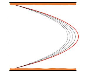
As expected, the overall effect translates into an extra viscous resistance which dampens down the velocity's distribution, more and more with increasing $\sigma ^2_Y$ (figure 2). Likewise, the mean velocity $V^\star$ results from the homogeneous one, i.e. $V$, as follows:

(4.5)\begin{equation} V^\star= \frac{V}{1 + \sigma^2_Y} =\frac{\mathcal{J} \rho g b^2}{12 \mu ( 1 + \sigma^2_Y)}. \end{equation}

By the same token, one can compute the friction coefficient $\lambda ^\star$. More precisely, substitution of (4.5) in the Darcy–Weisbach law, i.e. $\lambda = c_f \mu / ( \rho V \ell )$ (being, for the problem at stake, $c_f = 96$ whereas $\ell$ is a characteristic length scale), leads to

(4.6)\begin{equation} \lambda^\star= \frac{96 \mu}{\rho V \ell} ( 1 + \sigma^2_Y ) = \frac{96}{Re^\star}, \quad {Re}^\star= \frac{Re}{1 + \sigma^2_Y}. \end{equation}

Like above, the friction coefficient $\lambda ^\star$ is obtained by replacing the homogeneous Reynolds number, i.e. ${Re} = \rho V \ell / \mu$, with its modified version, i.e. ${Re}^\star$. Any increase in the degree of irregularity (i.e. $\sigma ^2_Y$) in the wall's geometry generates a larger friction (for fixed velocity distribution). Finally, unlike $\bar {\boldsymbol {v}}$, the pressure $p$ is not affected by the wall's geometry. This is explained by noting that $p$ obeys Stevin's law, and therefore it is not affected by the fluid's viscosity.

Figure 2. Non-dimensional velocity's profile $\mu v^1_{(0)} / ( \mathcal {J} \rho g b^2 )$ as affected by different degrees of the roughness’ heterogeneity. Red thick line corresponds to the homogeneous solution (3.9).

The aim of the present study was to develop a procedure of solving Stokes flow between two parallel plates which, unlike the homogeneous case, here exhibit an irregular geometry. The spatial distribution of the latter is regarded as a stationary, log-normal, random field. We present a new methodology which allows mapping the actual domain upon another one of regular boundaries. The utility of such a procedure relies upon the fact that now the random nature of the signal characterizing the walls’ topology is encompassed in the transformed stochastic equations, that can be solved by means of standard (either numerical or analytical) tools. In particular, we develop a model of the mean flow variables by regarding the variance of the log-transform of the above signal as a small parameter.

The main result of our study is an effective Poiseuille-type equation relating the mean velocity to the mean pressure. The tensor multiplying the Laplacian of the mean velocity is coined as effective viscosity and, unlike its homogeneous counterpart, it cannot anymore be regarded as a fluid's property, solely. In particular, it is shown that one can still use the classical Hagen–Poiseuille solution provided that the fluid's viscosity is replaced with the effective one. Moreover, the present study also lends itself as a tool to identify the main features of the roughness, by matching measurements of the flow variables (such as the velocity) and/or the viscosity against the analytical model. To conclude, the stochastic mapping that we have presented finds application to predict a bulk flow in a plane channel, given the parameters describing the geometry of the walls.

Acknowledgements

The constructive comments from two anonymous referees have been deeply appreciated, and they have significantly improved the early version of the manuscript.

Funding

This work was supported in part by the Departmental fund – project 3778/2022; and by the Italian Ministry of University and Research (PRIN) under grant P2022WC2ZZ.

Declaration of interests

The author reports no conflict of interest.

Appendix A. Second-order correction

The ensemble average of (3.7) with $n=2$ is

(A1)\begin{equation} \left.\begin{array}{c@{}} \nabla^2 \bar v^i_{(2)} - \dfrac{\partial \bar h_{(2)} }{\partial \xi^i} = \bar{\mathcal{F}}^i_{(2)},\\ \boldsymbol{\nabla} \boldsymbol{\cdot} \bar{\boldsymbol{v}}_{(2)} = \bar{\mathcal{Q}}_{(2)}. \end{array}\right\} \end{equation}

To compute the ensemble average $\mathbb {E}\{ \mathcal {F}_{(2)}^i \} \equiv \bar { \mathcal {F}}_{(2)}^i$, we rewrite $\mathcal {F}_{(2)}^i$ in (3.7c) as

(A2)\begin{equation} \mathcal{F}_{(2)}^i = \mathcal{G}^{i1}_{(2)} \dfrac{\partial h_{(0)}}{\partial \xi^1} + \mathcal{G}^{ik}_{(1)} [ \nabla^2 v^k_{(1)} - \mathcal{F}^k_{(1)} ] - \dfrac{\partial}{\partial \xi^j} \left[ \mathcal{G}^{jk}_{(2)} \dfrac{\partial v^i_{(0)}}{\partial \xi^k} + \mathcal{G}^{jk}_{(1)} \dfrac{\partial v^i_{(1)}}{\partial \xi^k} \right] \end{equation}

or, accounting for (3.9) and (3.7) with $n=1$, as

(A3)\begin{equation} \mathcal{F}_{(2)}^i = \mathcal{J} \mathcal{G}^{i1}_{(2)} - \dfrac{\partial}{\partial \xi^j} \left ( \mathcal{G}^{jk}_{(2)} \dfrac{\partial v^i_{(0)}}{\partial \xi^k} \right) - \mathcal{G}^{ik}_{(1)} \mathcal{F}^k_{(1)} + \mathcal{G}^{ik}_{(1)} \nabla^2 v^k_{(1)} - \dfrac{\partial}{\partial \xi^j} \left( \mathcal{G}^{jk}_{(1)} \dfrac{\partial v^i_{(1)}}{\partial \xi^k} \right). \end{equation}

Since $\mathbb {E} \{ \mathcal {G}^{ij}_{(2)} \} = \delta ^i_j \sigma ^2_Y / 2$, the ensemble average of this expression yields

(A4)\begin{equation} \bar{\mathcal{F}}_{(2)}^i = \delta^i_1 \mathcal{J} \frac{\sigma^2_Y}{2} + \delta^i_1 \mathcal{J} \frac{\sigma^2_Y}{2} - \mathbb{E} \left\{ \mathcal{G}^{ik}_{(1)} \mathcal{F}^k_{(1)} - \mathcal{G}^{ik}_{(1)} \nabla^2 v^k_{(1)} + \dfrac{\partial}{\partial \xi^j} \left( \mathcal{G}^{jk}_{(1)} \dfrac{\partial v^i_{(1)}}{\partial \xi^k} \right) \right\}. \end{equation}

It follows from (3.7b) and (3.8) that

(A5ac)\begin{equation} \mathcal{F}_{(1)}^1 ={-} 2 \mathcal{J} Y - \frac{\partial \mathcal{G}^{k3}_{(1)}}{\partial \xi^k} \frac{\partial v^1_{(0)}}{\partial \xi^3}, \quad \mathcal{F}_{(1)}^2 = 0, \quad \mathcal{F}_{(1)}^3 = \mathcal{J} \mathcal{G}^{31}_{(1)}. \end{equation}

Combining these expressions with those for $\mathcal {G}^{ik}_{(1)}$ in (3.8) and taking the ensemble average yields

(A6)\begin{equation} \mathbb{E} \{ \mathcal{G}^{ik}_{(1)} \mathcal{F}^k_{(1)} \} = 2 \mathcal{J} \sigma^2_Y \delta^i_1 . \end{equation}

In order to simplify the required mathematical burden to compute the ensemble average of the last two terms in (A4), hereafter the analysis is restricted to random fields $\gamma \equiv Y$, $\zeta$ characterized by a long range of correlation. This implies that the integral scale of $\gamma$ can be regarded as unbounded, and the same is valid for the integral length scale of the velocity's fluctuation since, within the perturbation expansion employed in the present study, one has $v^i_{(1)} = O ( \gamma )$. As a consequence, the velocity's fluctuation is scarcely varying in the space, and therefore its derivatives can be neglected. Hence, one finally ends up with $\bar { \mathcal {F}}_{(2)}^i = - \mathcal {J} \sigma ^2_Y \delta ^i_1$. A similar argument leads to $\bar {\mathcal {Q}}_{(2)} = 0$. Finally, for the deterministic externally imposed pressure gradient $\mathcal {J}$, $\boldsymbol {\nabla } \bar h = (\mathcal {J}, 0,0)^\top = \boldsymbol {\nabla } \bar h_{(0)}$, i.e. $\boldsymbol {\nabla } \bar h_{(2)} = \textbf{0}$. This leads to (3.10).

References

Arfken, G.B. & Weber, H.J. 2005 Mathematical Methods for Physicists, 6th edn. Academic.Google Scholar
Bahrami, M.M., Yovanovich, M.M. & Culham, J.R. 2006 a Pressure drop of fully-developed, laminar flow in microchannels of arbitrary cross-section. ASME J. Fluids Engng 128 (5), 10361044.CrossRefGoogle Scholar
Bahrami, M.M., Yovanovich, M.M. & Culham, J.R. 2006 b Pressure drop of fully developed, laminar flow in rough microtubes. ASME. J. Fluids Engng 128 (1), 632637.CrossRefGoogle Scholar
Brown, S.R. 1987 Fluid flow through rock joints: the effect of surface roughness. J. Geophys. Res. Solid Earth 92 (B2), 13371347.CrossRefGoogle Scholar
Brown, S.R. 1989 Transport of fluid and electric current through a single fracture. J. Geophys. Res. Solid Earth 94 (B7), 94299438.CrossRefGoogle Scholar
Brown, S.R., Stockman, H.W. & Reeves, S.J. 1995 Applicability of the Reynolds equation for modeling fluid flow between rough surfaces. Geophys. Res. Lett. 22 (18), 25372540.CrossRefGoogle Scholar
Chen, Y., Zhang, C., Shi, M. & Peterson, G.P. 2009 Role of surface roughness characterized by fractal geometry on laminar flow in microchannels. Phys. Rev. E 80 (2), 026301.CrossRefGoogle ScholarPubMed
Dewangan, M.K. 2024 Investigation of Stokes flow in a grooved channel using the spectral method. Theor. Comput. Fluid Dyn. 38 (1), 3959.CrossRefGoogle Scholar
Gamrat, G., Favre-Marinet, M., Le Person, S., Baviere, R. & Ayela, F. 2008 An experimental study and modelling of roughness effects on laminar flow in microchannels. J. Fluid Mech. 594, 399423.CrossRefGoogle Scholar
Herwig, H., Gloss, D. & Wenterodt, T. 2008 A new approach to understanding and modelling the influence of wall roughness on friction factors for pipe and channel flows. J. Fluid Mech. 613 (1), 3553.CrossRefGoogle Scholar
Hightower, C.M., et al. 2011 Integration of cardiovascular regulation by the blood/endothelium cell-free layer. WIREs Syst. Biol. Med. 3 (4), 458470.CrossRefGoogle ScholarPubMed
Kandlikar, S.G., Schmitt, D., Carrano, A.L. & Taylor, J.B. 2005 Characterization of surface roughness effects on pressure drop in single-phase flow in minichannels. Phys. Fluids 17 (10), 100606.CrossRefGoogle Scholar
Kwon, C. & Tartakovsky, D.M. 2020 Modified immersed boundary method for flows over randomly rough surfaces. J. Comput. Phys. 406, 109195.CrossRefGoogle Scholar
Lenci, A., Méheust, Y., Putti, M. & Di Federico, V. 2022 Monte Carlo simulations of shear-thinning flow in geological fractures. Water Resour. Res. 58 (9), e2022WR032024.CrossRefGoogle Scholar
Li, H., Fu, P., Zhou, Z., Sun, W., Li, Y., Wu, J. & Dai, Q. 2022 Performing calculus with epsilon-near-zero metamaterials. Sci. Adv. 8, eabq6198.CrossRefGoogle ScholarPubMed
Maggiolo, D., Manes, C. & Marion, A. 2013 Momentum transport and laminar friction in rough-wall duct flows. Phys. Fluid 25 (9), 093603.CrossRefGoogle Scholar
Moody, L.F. 1944 Friction factors for pipe flow. Trans. ASME 66 (8), 671684.Google Scholar
Murthy, A.N., Duwensee, M. & Talke, F.E. 2010 Numerical simulation of the head/disk interface for patterned media. Tribol. Lett. 38, 4755.CrossRefGoogle Scholar
Navajas, D., Pérez-Escudero, J.M., Martínez-Hernández, M.E., Goicoechea, J. & Liberal, I. 2023 Addressing the impact of surface roughness on epsilon-near-zero silicon carbide substrates. ACS Photonics 10, 31053114.CrossRefGoogle ScholarPubMed
Nawaz, H., Masood, M.U., Saleem, M.M., Iqbal, J. & Zubair, M. 2020 Surface roughness effects on electromechanical performance of RF-MEMS capacitive switches. Microelectron. Reliab. 104, 113544.CrossRefGoogle Scholar
Owen, D.G., Schenkel, T., Shepherd, D.E.T. & Espino, D.M. 2020 Assessment of surface roughness and blood rheology on local coronary haemodynamics: a multi-scale computational fluid dynamics study. J. R. Soc. Interface 17 (169), 20200327.CrossRefGoogle ScholarPubMed
Park, S.-W., Intaglietta, M. & Tartakovsky, D.M. 2012 Impact of endothelium roughness on blood flow. J. Theor. Biol. 300, 152160.CrossRefGoogle ScholarPubMed
Park, S.-W., Intaglietta, M. & Tartakovsky, D.M. 2015 Impact of stochastic fluctuations in the cell free layer on nitric oxide bioavailability. Front. Comput. Neurosci. 9, 131.CrossRefGoogle ScholarPubMed
Plouraboué, F., Geoffroy, S. & Prat, M. 2004 Conductances between confined rough walls. Phys. Fluids 16 (3), 615624.CrossRefGoogle Scholar
Severino, G. & De Bartolo, S. 2015 Stochastic analysis of steady seepage underneath a water-retaining wall through highly anisotropic porous media. J. Fluid Mech. 778, 253272.CrossRefGoogle Scholar
Severino, G., Giannino, F., De Paola, F. & Di Federico, V. 2023 Effective conductivity of inertial flows through porous media. Phys. Rev. E 107, 035102.CrossRefGoogle ScholarPubMed
Tartakovsky, D.M. & Xiu, D. 2006 Stochastic analysis of transport in tubes with rough walls. J. Comput. Phys. 217 (1), 248259.CrossRefGoogle Scholar
Tavakol, B., Froehlicher, G., Holmes, D.P. & Stone, H.A. 2017 Extended lubrication theory: improved estimates of flow in channels with variable geometry. Proc. R. Soc. A 473 (2206), 20170234.CrossRefGoogle ScholarPubMed
Viswanathan, H.S., et al. 2022 From fluid flow to coupled processes in fractured rock: recent advances and new frontiers. Rev. Geophys. 60 (1), e2021RG000744.CrossRefGoogle Scholar
Wang, X.-Q., Yap, C. & Mujumdar, A.S. 2005 Effects of two-dimensional roughness in flow in microchannels. J. Electron. Packag. 127 (3), 357361.CrossRefGoogle Scholar
Webb, R.L. & Kim, N.-H. 1994 Principles of Enhanced Heat Transfer. Taylor Francis.Google Scholar
Xiu, D. & Tartakovsky, D.M. 2006 Numerical methods for differential equations in random domains. SIAM J. Sci. Comput. 28 (3), 11671185.CrossRefGoogle Scholar
Yaglom, A.M. 1987 Correlation Theory of Stationary and Related Random Functions. I. Basic Results. Springer.Google Scholar
Yamane, R., Mori, S., Arakawa, M., Wilhjelm, J.E. & Kanai, H. 2023 Ultrasonic measurement of carotid luminal surface roughness with removal of axial displacement caused by blood pulsation. Japan. J. Appl. Phys. 62, SJ1042.CrossRefGoogle Scholar
Yi, J., Tian, F.-B., Simmons, A. & Barber, T. 2022 Impact of modelling surface roughness in an arterial stenosis. Fluids 7 (5), 179.CrossRefGoogle Scholar
Zayernouri, M., Park, S.-W., Tartakovsky, D.M. & Karniadakis, G.E. 2013 Stochastic smoothed profile method for modeling random roughness in flow problems. Comput. Meth. Appl. Mech. Engng 263, 99112.CrossRefGoogle Scholar
Zheng, Z., Valdebenito, M., Beer, M. & Nackenhorst, U. 2023 A stochastic finite element scheme for solving partial differential equations defined on random domains. Comput. Meth. Appl. Mech. Engng 405, 115860.CrossRefGoogle Scholar
Figure 0

Figure 1. Frontal (i) and longitudinal (ii) views of two parallel plates (aperture $b$) hosting the flow. The domain is such that $( x_1, x_2 ) \in \mathbb {R}^2$, whereas the vertical coordinate $x_3 \in [z_{bot}, z_{top}]$ is bounded between the top and bottom irregular surfaces (orange face).

Figure 1

Figure 2. Non-dimensional velocity's profile $\mu v^1_{(0)} / ( \mathcal {J} \rho g b^2 )$ as affected by different degrees of the roughness’ heterogeneity. Red thick line corresponds to the homogeneous solution (3.9).