


1. Introduction
Ocean mesoscale eddies play an essential role in water exchange and material circulation. In particular, western boundary regions are well known as areas with western boundary currents characterized by eddy activity, with oceanic eddy termination frequently occurring because the eddies tend to move westward (Chelton, Schlax & Samelson Reference Chelton, Schlax and Samelson2011). Since oceanic eddies transport momentum, heat and water masses, investigating their behaviour is essential for understanding the ocean environment and its variability in the western region (Spall et al. Reference Spall, Pickart, Fratantoni and Plueddemann2008; Chelton et al. Reference Chelton, Schlax and Samelson2011; Baird & Ridgway Reference Baird and Ridgway2012; Dong et al. Reference Dong, McWilliams, Liu and Chen2014). Western ocean regions have distinct topography, including continental shelves/slopes. Since distinct topography can play an essential role in the evolution of eddies, the investigation of eddy–topography interactions is critical for understanding the material transport via the movement of eddies (Spall et al. Reference Spall, Pickart, Fratantoni and Plueddemann2008; Itoh & Yasuda Reference Itoh and Yasuda2010; Ribbe et al. Reference Ribbe, Toaspern, Wolff and Azis Ismail2018).
A characteristic phenomenon in western boundary regions is that anticyclonic eddies propagate poleward along the coast. On the eastern coast of Japan, Kuroshio warm-core rings have been observed to propagate north (Yasuda, Okuda & Hirai Reference Yasuda, Okuda and Hirai1992; Kaneko et al. Reference Kaneko, Itoh, Kouketsu, Okunishi, Hosoda and Suga2015). In the South Pacific, many observations have shown that anticyclonic eddies that form off the eastern coast of Australia move poleward along the western boundary (Schaeffer et al. Reference Schaeffer, Gramoulle, Roughan and Mantovanelli2017; Azis Ismail & Ribbe Reference Azis Ismail and Ribbe2019). Itoh & Sugimoto (Reference Itoh and Sugimoto2001) numerically reproduced the poleward movement of an eddy that was initially near the topography using primitive equations and found that the effect of the steep bottom slope was an important factor in this motion.
In the open ocean, eddies largely propagate west due to the  $\beta$-effect; once eddies reach the western boundary, they typically move along that boundary as if they are trapped. However, there is an eastward-propagating solution with a dipole structure. This structure is known as a modon (Stern Reference Stern1975; Flierl et al. Reference Flierl, Larichev, McWilliams and Reznik1980). Hughes & Miller (Reference Hughes and Miller2017) recently observed modons moving eastward in the Tasman Sea using satellite altimeter data and suggested that the bottom topography could play an important role in the formation process. While the modon is a solution consisting of two vortices in the same density layer, a dipole structure with eddies in different layers is also possible. This type of structure is known as a heton (Hogg & Stommel Reference Hogg and Stommel1985). Since hetons have high heat and material transport capabilities, they are thought to be significant structures in the ocean (Richardson & Tychensky Reference Richardson and Tychensky1998; Morel & McWilliams Reference Morel and McWilliams2001; Serra & Ambar Reference Serra and Ambar2002; Carton et al. Reference Carton, Daniault, Alves, Cherubin and Ambar2010; Serra, Ambar & Boutov Reference Serra, Ambar and Boutov2010).
Several studies have used idealized models to investigate the interaction between eddies and the bottom topography (Wang Reference Wang1991; McDonald Reference McDonald1998; Dunn, McDonald & Johnson Reference Dunn, McDonald and Johnson2001; White & McDonald Reference White and McDonald2004; Baker-Yeboah et al. Reference Baker-Yeboah, Flierl, Sutyrin and Zhang2010; Zhang, Pedlosky & Flierl Reference Zhang, Pedlosky and Flierl2011; de Marez et al. Reference de Marez, Carton, Morvan and Reinaud2017). McDonald (Reference McDonald1998) and Dunn et al. (Reference Dunn, McDonald and Johnson2001) studied the motion of a point vortex near a step-like topography in a 1.5-layer quasi-geostrophic model in the  $f$-plane. McDonald (Reference McDonald1998) found that intense vortices cause a potential vorticity front, which is located along the topography, to wrap around themselves. They defined an intense vortex as one in which the time scale for vortex circulation,
  $T_a$, is much shorter than the time scale for topographic wave generation,
  $T_w$. Dunn et al. (Reference Dunn, McDonald and Johnson2001) investigated moderate,
  $T_w\approx T_a$, and weak,
  $T_w \ll T_a$, point vortices. They found that a moderate vortex forms a dipole structure consisting of a point vortex and the vortex caused by potential vorticity conservation, while a weak vortex propagates steadily along the topography. They analytically showed that a weak vortex propagates parallel to the topography. They referred to this phenomenon as the pseudoimage of the vortex and derived its linear solution. Other studies have also confirmed that the interaction of a vortex with a step-like topography causes propagating vortices along the topography and the formation of dipole structures (Dunn Reference Dunn2002; Dunn, McDonald & Johnson Reference Dunn, McDonald and Johnson2002; White & McDonald Reference White and McDonald2004).
Previous studies focused solely on situations in which vortices were located in the same layer as the topography. However, the interaction between an upper-layer vortex and a lower-layer topography is important to consider for oceanic applications because of density stratification in real environments. Moreover, it is reasonable to hypothesize that the distance between the topography and the vortex is an important parameter for controlling the system. However, the dependence of this parameter on vortex motion is still unclear. Therefore, we investigated the interaction between the upper vortex and the lower step-like topography using a two-layer quasi-geostrophic model in an  $f$-plane. The purpose of the present study is to clarify the types of motion that occur in this system and the properties of each motion type.
After formulating the problem in § 2, we show the analytical results based on linear theory at the limit of a weak point vortex in § 3. A finite-amplitude pseudoimage solution is derived in § 4. In § 5, we numerically investigate the temporal evolution of both the pseudoimage solution and the system. The conclusions are presented in § 6.
2. Model formulation
2.1. Potential vorticity and point vortex equations
In the present study, we used a two-layer quasi-geostrophic model in the  $f$-plane, with the point vortex in the upper layer and the step-like topography in the lower layer (see figure 1). Our model has two layers with an average thickness of
  $H_j$ and a density of
  $\rho _j$, where
  $j=1, 2$ denotes the upper and lower layers, respectively. The density in each layer is written in terms of the reference density of the fluid,
  $\rho _0$, and the density difference between the two layers,
  ${\rm \Delta} \rho$, as
  $\rho _1=\rho _0$ and
  $\rho _2=\rho _0+{\rm \Delta} \rho$. The point vortex in the upper layer has a circulation of
  $\varGamma$ and is located at a distance of
  $Y_0$ from the topography. In the lower layer,
  $h_B$, which denotes the bottom topography, is written as
  $h_B=-{\rm \Delta} H \mathrm {sgn}(y)$, where
  ${\rm \Delta} H$ is the amplitude of the bottom topography and
  $\mathrm {sgn}(y)$ is the sign function. Assuming that
  ${\rm \Delta} H/H_2 \ll 1$, we can use the quasi-geostrophic approximation to formulate this system. The governing equation and the quasi-geostrophic potential vorticity,
  $q_j$, in each layer can be written in non-dimensional forms as
 $$\begin{gather} \frac{\partial q_j}{\partial t}+J(\psi_j,q_j)=0, \end{gather}$$
 $$\begin{gather}q_1=\nabla^2 \psi_1 -\gamma_L \psi_1-(\psi_1-\psi_2), \end{gather}$$
 $$\begin{gather}q_2=\nabla^2 \psi_2 +\gamma_H(\psi_1-\psi_2)+h_B, \end{gather}$$
where  $t$ is the time,
  $J$ is the Jacobian and
  $\psi _j$ is the streamfunction in the
  $j$th layer. The equations in this system were non-dimensionalized using the length scale
  $L=\sqrt {g^\prime H_1}/f$ and the time scale
  $T= (f {\rm \Delta} H/H_2)^{-1}$, where
  $g^{\prime }$ is the reduced gravity and
  $f$ is the Coriolis parameter. We scaled the relative vorticity by
  $T^{-1}=f {\rm \Delta} H/H_2$ and the streamfunctions by
  $L^2 T^{-1}=(g^\prime H_1/f)({\rm \Delta} H/H_2)$. The non-dimensional amplitude of the point vortex circulation is
  $\varepsilon =|\varGamma |T/L^2=|\varGamma |f/(g^\prime H_1)/({\rm \Delta} H/H_2)$. The remaining non-dimensional parameters in the equations are
  $\gamma _H=H_1/H_2$ and
  $\gamma _L={\rm \Delta} \rho /\rho _0$. In addition to these non-dimensional parameters, the initial
  $y$-coordinate of the point vortex,
  $Y_0$, contributes to the behaviour of this system. Also,
  $Y_0$ is non-dimensionalized by
  $L$. It should be noted that the streamfunction in the
  $j$th layer is invariant under the transformation
  $\psi _j(x,y) \to -\psi _j(x,-y)$.

Figure 1. Schematic illustration of the model configuration. (a) The cross-section of the two-layer fluid. (b) The initial condition for this problem. The point vortex indicated by  $\ast$ is located at
  $y=Y_0$ and has a circulation of
  $\varGamma$.
Our model has a point vortex in the upper layer and a potential vorticity front that initially lies along the step-like topography,  $y=0$, in the lower layer. Based on the locations of the point vortex,
  $(X(t), Y(t))$, and the potential vorticity front,
  $y=\eta (t,x)$, we can write the non-dimensional potential vorticity in each layer as
 $$\begin{gather} q_1=\varepsilon \mathrm{sgn}(\varGamma)\delta(x-X,y-Y), \end{gather}$$
 $$\begin{gather}q_2={-}\mathrm{sgn}(y-\eta). \end{gather}$$
The velocity caused by the topography can be determined based on the potential vorticity anomaly in the lower layer,  ${\rm \Delta} q_2$. This anomaly occurs because of the displacement between the potential vorticity front and the topography and is given by
 \begin{equation}
{\rm \Delta} q_2=\left\{\begin{array}{@{}ll} +2, & 0< y<\eta\\ -2,
& \eta< y<0\\ 0, & \mbox{otherwise} \end{array}\right..
\end{equation}
\begin{equation}
{\rm \Delta} q_2=\left\{\begin{array}{@{}ll} +2, & 0< y<\eta\\ -2,
& \eta< y<0\\ 0, & \mbox{otherwise} \end{array}\right..
\end{equation}
In terms of  $\eta (t,x)$,
  $X(t)$ and
  $Y(t)$, the governing equation in this system can be written as
 $$\begin{gather} \frac{\partial \eta}{\partial t}+u_2(t,x,\eta) \frac{\partial \eta}{\partial x}=v_2(t,x,\eta), \end{gather}$$
 $$\begin{gather}\frac{\mathrm{d}X}{\mathrm{d}t}=u_1(t,X,Y),\quad \frac{\mathrm{d}Y}{\mathrm{d}t}=v_1(t,X,Y), \end{gather}$$
where  $u_j$ and
  $v_j$ are the horizontal components of the velocity and are given by
 \begin{equation} u_j={-}\frac{\partial \psi_j}{\partial y},\quad v_j=\frac{\partial \psi_j}{\partial x}. \end{equation}
The streamfunction is determined by the equations
 \begin{equation}
\nabla^2 \left(\begin{array}{@{}c@{}} \psi_1 \\ \psi_2
\end{array}\right) -\boldsymbol{\mathsf{M}} \left(\begin{array}{@{}c@{}} \psi_1 \\
\psi_2 \end{array}\right) =\left(\begin{array}{@{}c@{}}
\varepsilon \mathrm{sgn}(\varGamma) \delta(x-X,y-Y)\\
{\rm \Delta} q_2 \end{array}\right),
\end{equation}
\begin{equation}
\nabla^2 \left(\begin{array}{@{}c@{}} \psi_1 \\ \psi_2
\end{array}\right) -\boldsymbol{\mathsf{M}} \left(\begin{array}{@{}c@{}} \psi_1 \\
\psi_2 \end{array}\right) =\left(\begin{array}{@{}c@{}}
\varepsilon \mathrm{sgn}(\varGamma) \delta(x-X,y-Y)\\
{\rm \Delta} q_2 \end{array}\right),
\end{equation}
written in vector form, where the coefficient matrix,  $\boldsymbol{\mathsf{M}}$, can be written as
 \begin{equation}
\boldsymbol{\mathsf{M}}=\left(\begin{array}{@{}cc@{}} \gamma_L+1 & -1\\ -\gamma_H &
\gamma_H \end{array}\right).
\end{equation}
\begin{equation}
\boldsymbol{\mathsf{M}}=\left(\begin{array}{@{}cc@{}} \gamma_L+1 & -1\\ -\gamma_H &
\gamma_H \end{array}\right).
\end{equation}2.2. Vertical mode decomposition
The streamfunctions in each layer can be decomposed into vertical modes. The eigenvalues and eigenvectors of  $\boldsymbol{\mathsf{M}}$ are denoted by
  $\lambda _\pm$ and
  $\boldsymbol{V}_\pm =(U_\pm,V_\pm )$, which can be written as
 $$\begin{gather} \lambda_\pm = \frac{1+\gamma_L+\gamma_H\pm \sqrt{(1+\gamma_L+\gamma_H)^2-4 \gamma_H \gamma_L}}{2}, \end{gather}$$
 $$\begin{gather}\boldsymbol{V}_\pm = (U_\pm,V_\pm)=\left(1,\frac{1+\gamma_L-\lambda_\pm}{\gamma_H}\right). \end{gather}$$
We note that the quantities  $\lambda _{+}^{-1/2}$ and
  $\lambda _{-}^{-1/2}$ correspond to the non-dimensional internal and external Rossby radii of deformation, respectively. We can define the streamfunctions of the
  $+$ and
  $-$ modes as
 \begin{equation} \psi_{{\pm}}=U_{{\pm}}\psi_1+V_{{\pm}}\psi_2. \end{equation}
By substituting (2.14) into (2.10) and using Green's function, we can write  $\psi _{\pm }$ as
 \begin{equation} \psi_\pm(t,x,y)=U_\pm \varepsilon \textrm{sgn}(\varGamma)G_\pm (x,X,y,Y)+2V_\pm \int_{-\infty}^{\infty} \mathrm{d}\kern0.06em x^\prime\int_{0}^{\eta(t,x^\prime)} \mathrm{d}y^\prime G_\pm(x,x^\prime,y,y^\prime), \end{equation}
where the Green's function in each mode,  $G_\pm$, is given by
 \begin{equation} G_\pm(x,x^\prime,y,y^\prime)={-}\frac{1}{2{\rm \pi}}K_0\left( \sqrt{\lambda_\pm} \sqrt{(x-x^\prime)^2+(y-y^\prime)^2}\right). \end{equation}
The streamfunction in each layer,  $\psi _j$, can be obtained from (2.14) and (2.16). We can decompose the streamfunction
  $\psi _j$ into the point vortex effect,
  $\varPsi _j$, and the topographic effect,
  $\phi _j$. According to (2.16) and (2.15), the streamfunctions caused by the point vortex can be written as
 $$\begin{gather} \varPsi_1=\frac{-\varepsilon \textrm{sgn}(\varGamma)}{V_-{-}V_+} \left\{V_+G_-(x,X,y,Y)-V_- G_+(x,X,y,Y)\right\}, \end{gather}$$
 $$\begin{gather}\varPsi_2=\frac{ \varepsilon \textrm{sgn}(\varGamma)}{V_-{-}V_+}\left\{G_-(x,X,y,Y)-G_+(x,X,y,Y)\right\} , \end{gather}$$
while those caused by the topography can be written as
 $$\begin{gather} \phi_1=\frac{2V_+ V_-}{V_-{-}V_+}\int_{-\infty}^{\infty} \mathrm{d}\kern0.06em x^\prime \int_{0}^{\eta(t,x^\prime)} \mathrm{d}y^\prime \left\{ G_-(x,x^\prime,y,y^\prime)-G_+(x,x^\prime,y,y^\prime)\right\}, \end{gather}$$
 $$\begin{gather}\phi_2=\frac{2}{V_-{-}V_+}\int_{-\infty}^{\infty} \mathrm{d}\kern0.06em x^\prime \int_{0}^{\eta(t,x^\prime)} \mathrm{d}y^\prime \left\{V_-G_-(x,x^\prime,y,y^\prime)-V_+G_+(x,x^\prime,y,y^\prime)\right\} , \end{gather}$$
where  $U_\pm =1$.
2.3. Contour dynamics
The flow field in this system is given by (2.9a,b) and (2.17)–(2.20). The horizontal velocity in the  $j$th layer,
  $\boldsymbol {u}_j=(u_j,v_j)$, is the sum of the velocity due to the point vortex,
  $\boldsymbol {u}^p_j$, and the velocity due to the topography,
  $\boldsymbol {u}^t_j$. According to (2.17) and (2.18), the velocity in the upper layer due to the point vortex can be written as
 $$\begin{gather} u^p_1(t,x,y)=\frac{\varepsilon \textrm{sgn}(\varGamma)}{V_-{-}V_+}\left\{V_+\frac{\partial G_-}{\partial y} (x,X,y,Y)-V_-\frac{\partial G_+}{\partial y} (x,X,y,Y)\right\}, \end{gather}$$
 $$\begin{gather}v^p_1(t,x,y)={-}\frac{\varepsilon \textrm{sgn}(\varGamma)}{V_-{-}V_+}\left\{V_+\frac{\partial G_-}{\partial x} (x,X,y,Y)-V_-\frac{\partial G_+}{\partial x} (x,X,y,Y)\right\}, \end{gather}$$
while the velocity in the lower layer due to the point vortex can be written as
 $$\begin{gather} u^p_2(t,x,y)={-}\frac{\varepsilon \textrm{sgn}(\varGamma)}{V_-{-}V_+}\left\{\frac{\partial G_-}{\partial y} (x,X,y,Y)-\frac{\partial G_+}{\partial y} (x,X,y,Y)\right\}, \end{gather}$$
 $$\begin{gather}v^p_2(t,x,y)=\frac{\varepsilon \textrm{sgn}(\varGamma)}{V_-{-}V_+}\left\{\frac{\partial G_-}{\partial x} (x,X,y,Y)-\frac{\partial G_+}{\partial x} (x,X,y,Y)\right\}. \end{gather}$$
According to (2.19) and (2.20), the velocity in the upper layer due to the topography can be written as
 \begin{align} u^t_1(t,x,y) &= \frac{2V_+V_-}{V_-{-}V_+} \int_{-\infty}^{\infty}\mathrm{d}\kern0.06em x^\prime \left\{ G_-(x,x^\prime,y,\eta)-G_+(x,x^\prime,y,\eta)\right., \nonumber\\ &\quad \left. -G_-(x,x^\prime,y,0)+G_+(x,x^\prime,y,0)\right\} \end{align}
 \begin{align} v^t_1(t,x,y)&=\frac{2V_+V_-}{V_-{-}V_+} \int_{-\infty}^{\infty}\mathrm{d}\kern0.06em x^\prime \left\{G_-(x,x^\prime,y,\eta)-G_+(x,x^\prime,y,\eta)\right\} \frac{\partial \eta}{\partial x^\prime}(t,x^\prime), \end{align}
while the velocity in the lower layer due to the topography can be written as
 \begin{align} u^t_2(t,x,y) &= \frac{2}{V_-{-}V_+} \int_{-\infty}^{\infty}\mathrm{d}\kern0.06em x^\prime \left\{ V_-G_-(x,x^\prime,y,\eta)-V_+G_+(x,x^\prime,y,\eta)\right., \nonumber\\ &\quad \left.-V_-G_-(x,x^\prime,y,0)+V_+G_+(x,x^\prime,y,0)\right\} \end{align}
 \begin{align} v^t_2(t,x,y)&=\frac{2}{V_-{-}V_+}\int_{-\infty}^{\infty}\mathrm{d}\kern0.06em x^\prime \left\{V_-G_-(x,x^\prime,y,\eta)-V_+G_+(x,x^\prime,y,\eta)\right\}\frac{\partial \eta}{\partial x^\prime}(t,x^\prime) . \end{align}
According to (2.7) and (2.8), we can determine the evolution of the system by using (2.23)–(2.28) to calculate the advection velocity at the front and at the point vortex.
The method of contour dynamics was used in this study to calculate the temporal evolution of the system (Zabusky, Hughes & Roberts Reference Zabusky, Hughes and Roberts1979). The contour dynamics method allows for an accurate treatment of inviscid fluid dynamics and has been used in numerous studies on the interaction between vortices and potential vorticity fronts (Stern & Flierl Reference Stern and Flierl1987; Bell Reference Bell1989; Wang Reference Wang1991; McDonald Reference McDonald1998; Dunn et al. Reference Dunn, McDonald and Johnson2001; Dunn Reference Dunn2002; White & McDonald Reference White and McDonald2004; Baker-Yeboah et al. Reference Baker-Yeboah, Flierl, Sutyrin and Zhang2010; Zhang et al. Reference Zhang, Pedlosky and Flierl2011).
3. Linear dynamics and pseudoimage solutions
3.1. Linearized equations
If we assume that the displacement of the potential vorticity front is small,  $|\eta | \ll 1$, and we maintain
  $|\eta |\ll 1$, we can also assume that
  $\varepsilon \le O(|\eta |)$. Then, the governing equation (2.7) becomes
 \begin{equation} \frac{\partial \eta}{\partial t}=v^p_2(t,x,0)+v^t_2(t,x,0), \end{equation}
where the  $O(|\eta |^2)$ terms are neglected. In this approximation, the velocities caused by the topography can be written as
 $$\begin{gather} u^t_1(t,x,y)=\frac{2V_-V_+}{V_-{-}V_+}\int_{-\infty}^{\infty}\mathrm{d}\kern0.06em x^\prime \left\{\frac{\partial G_-}{\partial y^\prime}(x,x^\prime,y,0)-\frac{\partial G_+}{\partial y^\prime} (x,x^\prime,y,0)\right\}\eta(t,x^\prime), \end{gather}$$
 $$\begin{gather}v^t_1(t,x,y)=\frac{2V_-V_+}{V_-{-}V_+}\int_{-\infty}^{\infty}\mathrm{d}\kern0.06em x^\prime \left\{ G_-(x,x^\prime,y,0)- G_+(x,x^\prime,y,0)\right\} \frac{\partial \eta}{\partial x^\prime}(t,x^\prime), \end{gather}$$
in the upper layer and
 $$\begin{gather} u^t_2(t,x,y)=\frac{2}{V_-{-}V_+}\int_{-\infty}^{\infty}\mathrm{d}\kern0.06em x^\prime \left\{V_-\frac{\partial G_-}{\partial y^\prime}(x,x^\prime,y,0)-V_+\frac{\partial G_+}{\partial y^\prime}(x,x^\prime,y,0)\right\}\eta(t,x^\prime), \end{gather}$$
 $$\begin{gather}v^t_2(t,x,y)=\frac{2}{V_-{-}V_+}\int_{-\infty}^{\infty}\mathrm{d}\kern0.06em x^\prime \left\{ V_- G_-(x,x^\prime,y,0)- V_+ G_+(x,x^\prime,y,0)\right\}\frac{\partial \eta}{\partial x^\prime}(t,x^\prime), \end{gather}$$
in the lower layer.
3.2. Linear topographic wave
In the absence of a point vortex, we examined the waves governed by linearized equations (3.1). Substituting the form of the wave solution,  $\eta =\hat {\eta }_0\exp \{\mathrm {i}(kx-\omega t)\}$, where
  $\hat {\eta }_0$ is a constant amplitude,
  $k$ is the wavenumber in the
  $x$-direction and
  $\omega$ is the frequency, into the governing equation, we obtain the condition for the existence of a non-trivial solution,
  $\hat {\eta }_0\ne 0$, as
 \begin{equation} \omega=\frac{k}{V_-{-}V_+}\left(\frac{V_-}{\sqrt{k^2+\lambda_-}}- \frac{V_+}{\sqrt{k^2+\lambda_+}}\right), \end{equation}
where we used both (2.16) and the relation
 \begin{equation} \int_{-\infty}^{\infty}\mathrm{d}\kern0.06em x\exp({-\mathrm{i}kx}) K_0\left(\sqrt{\lambda_\pm(x^2+y^2)}\right)= \frac{{\rm \pi}\exp({-|y|\sqrt{k^2+\lambda_\pm}})}{\sqrt{k^2+\lambda_\pm}}. \end{equation}
This relation (3.6) is the dispersion relation for linear topographic Rossby waves propagating along a step-like topography which has been derived by Rhines (Reference Rhines1977). According to (3.6), the phase speed and group velocity are
 $$\begin{gather} c=\frac{1}{V_-{-}V_+}\left(\frac{V_-}{\sqrt{k^2+\lambda_-}}-\frac{V_+}{\sqrt{k^2+\lambda_+}}\right), \end{gather}$$
 $$\begin{gather}c_g=\frac{1}{V_-{-}V_+}\left(\frac{\lambda_- V_-}{(k^2+\lambda_-)^{3/2}}-\frac{\lambda_+ V_+}{(k^2+\lambda_+)^{3/2}}\right), \end{gather}$$
respectively. Since  $\lambda _- < \lambda _+$ and
  $V_+< V_-$ hold for any value of
  $k$,
$k$,  $c$ and
  $c_g$ are always positive.
3.3. Linear pseudoimage solutions
In a previous study, Dunn et al. (Reference Dunn, McDonald and Johnson2001) used a 1.5-layer model to show the motion of a point vortex propagating steadily along a step-like topography and referred to this phenomenon as the pseudoimage of the vortex. In this study, we sought to determine the linear solution, referred to as the linear pseudoimage solution, and to investigate the properties of the solution.
To determine the steadily propagating solution of (3.1) that progresses with the point vortex, we assumed that the solution was in the form  $\eta =\eta (x-c_{pse}t)$, where the propagating speed,
  $c_{pse}$, is given as
  $c_{pse} \equiv \mathrm {d}X/\mathrm {d}t$. Since
  $\mathrm {d}X/\mathrm {d}t=u_1^t(t,X,Y)=O(\varepsilon )$, we can consider a situation in which the point vortex is fixed at
  $(0, Y_0)$. According to (3.1), the governing equation then becomes
 \begin{align} -c_{pse}\frac{\partial \eta}{\partial x} &= \frac{\partial \varPsi_2}{\partial x}(x,0)+ \frac{2}{V_-{-}V_+}\int_{-\infty}^{\infty}\mathrm{d}\kern0.06em x^\prime \left\{ V_-G_-(x,x^\prime,0,0)-V_+G_+(x,x^\prime,0,0)\right\} \nonumber\\ &\quad \times\frac{\partial \eta}{\partial x^\prime}(t,x^\prime), \end{align}
where  $v^p_2=\partial \varPsi _2/\partial x$. Although the term on the left side in the above equation has an order of
  $O(\varepsilon ^2)$, to investigate the asymmetry of the solution due to the sign of
  $c_{pse}$, we leave this term explicitly in the equation. Using both Fourier transform methods and (2.16) and (3.7), we can obtain the solution to (3.10) as
 \begin{equation} \eta(x-c_{pse})=\frac{1}{2{\rm \pi}}\int_{-\infty}^{\infty} \mathrm{d}k \frac{\exp({\mathrm{i}k(x-c_{pse}t)})}{c-c_{pse}}\mathcal{F}[\varPsi_2(x,0)], \end{equation}
where  $c$ is the phase speed of the topographic Rossby waves (3.8), and
  $\mathcal {F}[\varPsi _2]$ is the Fourier transform of
  $\varPsi _2$,
 \begin{equation} \mathcal{F}[\varPsi_2(x,0)]={-}\frac{1}{2}\frac{\varepsilon \mathrm{sgn}(\varGamma)}{V_-{-}V_+} \left\{\frac{\exp({-|Y_0|\sqrt{k^2+\lambda_-}})}{\sqrt{k^2+\lambda_-}}- \frac{\exp({-|Y_0|\sqrt{k^2+\lambda_+}})}{\sqrt{k^2+\lambda_+}}\right\}. \end{equation}
By substituting (3.11) into the linearized streamfunction caused by the topography,  $\phi _j$, we can obtain the linear pseudoimage solution in the two-layer model
 \begin{align} \phi_1 &= \frac{-1}{2{\rm \pi}}\frac{V_-V_+}{V_-{-}V_+} \int_{-\infty}^{\infty} \mathrm{d}k \frac{\exp({\mathrm{i}k(x-c_{pse}t)})}{c-c_{pse}} \nonumber\\ &\quad \times\left(\frac{\exp({-|y|\sqrt{k^2+\lambda_-}})}{\sqrt{k^2+\lambda_-}}- \frac{\exp({-|y|\sqrt{k^2+\lambda_+}})}{\sqrt{k^2+\lambda_+}}\right)\mathcal{F}[\varPsi_2(x,0)], \end{align}
 \begin{align} \phi_2&=\frac{-1}{2{\rm \pi}}\frac{1}{V_-{-}V_+} \int_{-\infty}^{\infty} \mathrm{d}k\frac{\exp({\mathrm{i}k(x-c_{pse}t)})}{c-c_{pse}} \nonumber\\ &\quad \times\left(\frac{V_-\exp({-|y|\sqrt{k^2+\lambda_-}})}{\sqrt{k^2+\lambda_-}}- \frac{V_+\exp({-|y|\sqrt{k^2+\lambda_+}})}{\sqrt{k^2+\lambda_+}}\right) \mathcal{F}[\varPsi_2(x,0)]. \end{align}
The propagating velocity,  $c_{pse}$, is given as
 \begin{align} c_{pse} &={-}\frac{\partial \phi_1}{\partial y}(0,Y_0)= \frac{\mathrm{sgn}(Y_0)}{2{\rm \pi}}\frac{V_-V_+}{V_-{-}V_+} \nonumber\\ &\quad \times\int_{-\infty}^{\infty} \mathrm{d}k \frac{\exp({-|Y_0|\sqrt{k^2+\lambda_-}})- \exp({-|Y_0|\sqrt{k^2+\lambda_+}})}{c-c_{pse}}\mathcal{F}[\varPsi_2(0,0)]. \end{align}
The sign of  $c_{pse}$ is equal to the sign of
  $Y_0 \varGamma$. The fields of the streamfunction,
  $\phi _j$ and
  $\phi _j+\varPsi _j$, are shown in figure 2. Although the
  $\phi _j$ field is similar to its counterpart in the 1.5-layer model, the
  $\phi _j+\varPsi _j$ field differs from its counterpart. In the 1.5-layer model, the fluid on the opposite side of the point vortex is at rest because the pseudoimage solution completely cancels any effects from the point vortex on this side. In a two-layer model, this cancellation is achieved only in the vicinity of the topography in the lower layer.

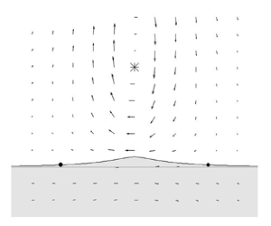
Figure 2. The  $\phi _j$ field (a,c) and the
  $\phi _j+\varPsi _j$ field (b,d) of the linear pseudoimage solution in the upper layer (a,b) and lower layer (c,d). The positive and negative streamlines are indicated by the solid and dashed lines, respectively. The positions of the maximum or minimum value are denoted by the cross. In the left panels, the contour interval is 0.005, and the minimum values are
  $-$0.0235 in the upper layer and
  $-$0.0292 in the lower layer. In the right panels, the contour interval is 0.001, and the maximum values are 0.0694 in the upper layer and 0.0098 in the lower layer. In all the cases shown here,
  $\mathrm {sgn}(\varGamma )=-1$,
  $\varepsilon =0.1$,
  $Y_0=1$,
  $\gamma _L=10^{-3}$ and
  $\gamma _H=1$. The point vortex is indicated by the closed circle at (0,1). The topography is located along
  $y=0$.
3.4. Small but non-zero amplitude pseudoimage solution
If we suppose that  $0<\varepsilon \ll 1$ but
  $\varepsilon$ is finite, we can examine the properties of a two-layer pseudoimage with a finite amplitude. In this parameter region,
  $\phi _j$ may have poles at the wavenumbers,
  $k_c$, that satisfy
  $c=c_{pse}$. The integrations (3.13) and (3.14) do not include
  $k_c$ when the point vortex moves in the opposite direction of the topographic waves, i.e.
  ${c_{pse}<0}$. In contrast, if
  $c_{pse}>0$, the solutions include a singularity because the path must contain
  $k_c$. In the 1.5-layer model, Dunn et al. (Reference Dunn, McDonald and Johnson2001) confirmed that a finite length wave train in the wake of the vortex is excited and that the point vortex drifts towards the topography due to the presence of the singularity. Similar behaviours are expected in the two-layer model. However, since the poles
  $k_c$ correspond to short waves, the singularity only has a small influence on the pseudoimage solution (see figure 3a).

Figure 3. (a) The dependencies of the wavenumbers,  $k_c$, which satisfy
  $c=c_{pse}$ on
  $\mathrm {sgn}(\varGamma )\varepsilon$ for
  $Y_0=1$ and are calculated from (3.8) and (3.15). Since
  $c$ is a function of
  $k^2$, there are both positive and negative
  $k_c$. As
  $\mathrm {sgn}(\varGamma ) \varepsilon \to 0$,
  $|k_c|$ diverges to infinity. (b) The dependence of the propagation velocity,
  $c_{pse}$, on
  $Y_0$. The propagation velocity has a maximum at approximately
  $Y_0=0.7$. In both panels,
  $\gamma _H=1$ and
  $\gamma _L=10^{-3}$.
Figure 3(b) shows the  $Y_0$ dependence of
  $c_{pse}$ in the parameter region
  $0<\varepsilon \ll 1$. The propagation speed,
  $|c_{pse}|$, does not monotonically decrease along
  $Y_0$, and it has an extreme value at
  $Y_0 \approx 0.7$. This corresponds to the radial distance in the lower layer where the upper-point vortex has its maximum azimuthal velocity, i.e. the internal Rossby radius of deformation,
  $\lambda _+^{-1/2} \approx 0.7$. Another feature is that
  $c_{pse}$ is non-singular as
  $Y_0 \to 0$. This non-singularity occurs because the lower layer lacks a singular point at the location of the point vortex.
4. Finite-amplitude pseudoimage solution
It is difficult to obtain analytical expressions for finite-amplitude, nonlinear solutions. In this section, we determined finite-amplitude steadily propagating solutions by numerically solving (2.7) with (2.21)–(2.28). According to the linear arguments, the finite-amplitude pseudoimage solutions can exist only when  $\mathrm {sgn}(\varGamma Y_0)=-1$. Hence, in this section, we focus on the case of an anticyclonic point vortex at the deeper side.
First, we use the Galilean transformation,
 \begin{equation} x \to \xi=x- c_{pse}t. \end{equation}
Then, the governing equation can be written as
 \begin{equation} -c_{pse} \frac{\partial \eta}{\partial \xi}+u_2\frac{\partial \eta}{\partial \xi}=v_2. \end{equation}
As a result, the pseudoimage solutions satisfy the equation
 \begin{equation} \frac{\partial \eta}{\partial \xi}=\frac{v_2}{u_2-c_{pse}}. \end{equation}
The boundary condition can be written as
 \begin{equation} \eta \rightarrow 0 \quad \mbox{as}\ |\xi| \rightarrow \infty. \end{equation}
Furthermore, we assume that the solution is symmetric with  $\xi =0$. Therefore, we have
 \begin{equation} \eta(-\xi)=\eta(\xi). \end{equation}
We compute  $\eta$ only for
  $\xi \le 0$.
To perform the numerical calculations, we discretize the potential vorticity front into  $N$ nodes for
  $-\xi _{\infty } \le \xi _n \le 0$, where
  $\xi _1=-\xi _{\infty }$ and
  $\xi _N=0$. Since the contribution of the far field is weak in the integration (2.28) and (2.29), the node spacing near the crest should be fine, whereas the spacing in the far field can be rough. Therefore, we set
  $\xi _n=\mu _0 (n-N)$ for
  $n \ge N_1$ and
  $\xi _n=-W+1-\mu _0(N_1-n)-\exp [\mu _0(N_1 -n)/5]$ for
  $n < N_1$, where
  $W=\mu _0 (N-N_1)$ and
  $\xi _\infty =W-1+\mu _0(N_1-1)+\exp [\mu _0(N_1-1)/5]$. In this study, we set
  $\mu _0=0.02,\ N=2650$ and
  $N_1=1150$; thus, we have
  $W=30$ and
  $\xi _\infty \simeq 151$. The finite-difference form of (4.3) is
 \begin{equation} \frac{\eta_{n+1}-\eta_{n-1}}{\xi_{n+1}-\xi_{n-1}}= \frac{v_{2,n}}{u_{2,n}-c_{pse}},\quad n=1,\ldots,2N-1. \end{equation}
The boundary conditions at  $\xi =\xi _1,\xi _N$ are
 $$\begin{gather} \eta_1=0, \end{gather}$$
 $$\begin{gather}\eta_N=\frac{\eta_{N-1}-\eta_{N-2}}{\xi_{N-1}-\xi_{N-2}}(\xi_N -\xi_{N-1})+\eta_{N-1} , \end{gather}$$
where (4.7) corresponds to (4.4), and (4.8) indicates that the front can be approximated as a quadratic function near the origin. As a result, we can obtain the frontal displacement,  $\eta _n$, and the propagation velocity,
  $c_{pse}$, for the given values of
  $\varepsilon$ by solving (4.6), (4.7), (4.8), with the condition that the solution propagates with the point vortex,
  $c_{pse}=u_1(0, Y_0)$, where the point vortex is located at
  $(0, Y_0)$. We used MINPACK (Moreé, Garbow & Hillstrom Reference Moreé, Garbow and Hillstrom1980) to solve the nonlinear simultaneous equations, with the front displacement of the linear solution (3.11) as the initial value in the iterative calculation. In this study, the midpoint method was used for the numerical integration. The validity of the obtained solutions was confirmed by conducting numerical experiments with the solutions as initial conditions. In the following subsections, we set the remaining parameter values as
  $\gamma _H=1$,
  $\gamma _L=10^{-3}$ and
  $Y_0=1$.
4.1. Dependency on  $\varepsilon$

Figure 4 shows the frontal displacement and propagation speeds for various values of  $\varepsilon$ obtained by solving the simultaneous equations. As
  $\varepsilon$ increases, both the displacement and the propagation speed,
  $|c_{pse}|$, increase. Figure 4(b) suggests that the linear solution is valid for small values of
  $\varepsilon$. Figure 5 shows that the nonlinearity sharpens the peak of the frontal displacement.

Figure 4. (a) The potential vorticity front and (b) its propagation speed for each value of  $\varepsilon$. Here,
  $\varepsilon$ ranges from 0.1 to 1 in steps of 0.1. The front with the maximum displacement was observed for
  $\varepsilon =1$. The propagation speed obtained by the linear solution is indicated by the dashed line in the right panel.

Figure 5. The potential vorticity front of the linear (dashed line) and nonlinear (solid line) solutions for  $\varepsilon =1$.
4.2. The saddle-node point
Figure 6 shows the current vectors caused by the frontal displacement and the point vortex in  $\xi$–
 $y$ coordinates. There are two saddle-node points in the front with
  $u_2-c_{pse}=0$. Since these points also exist when
  $\varepsilon$ is small, the existence of these points is believed to be a common feature of the pseudoimage solutions. The existence of this point may affect the time evolution of the front as in eddy–jet interactions (Bell & Pratt Reference Bell and Pratt1992; Capet & Carton Reference Capet and Carton2004); this will be investigated with numerical experiments in § 5.1.

Figure 6. The potential vorticity front of the nonlinear solution and the current vectors caused by the nonlinear solution and the point vortex in  $\xi$–
 $y$ coordinates. (a) Shows the case
  $\varepsilon =0.1$, and (b) shows the case
  $\varepsilon =1$. The closed circles on the front represent the saddle points.
5. Numerical experiments for nonlinear evolution
In this section, we perform numerical experiments. First, we consider the temporal evolution of the pseudoimage solution obtained in the previous section. Then, to investigate the temporal evolution of the system in the parameter space consisting of  $\varepsilon$ and
  $Y_0$, we perform numerical experiments with various initial conditions.
As in the previous section, we resolve the front into discrete nodes with positions  $(x_n, \eta _n)$. From the Lagrangian perspective, the temporal evolution of these nodes can be written as
 $$\begin{gather} \frac{\mathrm{d}\kern0.06em x_n}{\mathrm{d}t}=u_2(t,x_n,\eta_n), \end{gather}$$
 $$\begin{gather}\frac{\mathrm{d}\eta_n}{\mathrm{d}t}=v_2(t,x_n,\eta_n). \end{gather}$$
We can determine the temporal evolution of the system by calculating (2.8), (5.1) and (5.2). The velocities advecting the point vortex and the front can be evaluated numerically by calculating (2.21)–(2.28). The numerical integration scheme used to calculate the velocities is the same as in the previous section. The initial node distribution is the same as that in § 4. Since the front near the point vortex elongates with time in its evolution, a new node is added by linear interpolation to keep a spatial resolution when the distance between the adjacent nodes,  $\mu$, is
  $\mu >1.5 \mu _0$, where
  $\mu _0=0.02$. This interpolation is performed in the region of
  $|x| \leq W$ because the elongation of the front is negligibly small in the region of
  $|x|>W$, where
  $W=30$. When filamentation structures appear, the number of nodes in the front rapidly increases. To avoid calculating a large number of nodes, we use a contour surgery algorithm (Dritschel Reference Dritschel1988; Shimada & Kubokawa Reference Shimada and Kubokawa1997). In particular, we employ the algorithm described in Shimada & Kubokawa (Reference Shimada and Kubokawa1997). The validity of the predefined parameter
  $\mu _c$, the minimum distance between two segments on the front, was verified by comparing the area surrounded by the front and the topography in surgery and no-surgery experiments for several different parameters. The fourth-order Runge–Kutta method was used for time integration in the numerical experiments. The accuracy of the calculation was verified by comparing the phase speed of a small-amplitude sine wave in the absence of a point vortex calculated by the numerical experiment with the analytical result (3.8). All the numerical experiments in this section used
  $\gamma _L=10^{-3}$,
  $\gamma _H=1$,
  $\mu _c=0.002$ and a time step of
  ${\rm \Delta} t=0.01$. The parameters
  $\varepsilon$ and
  $Y_0$ are shown for each experiment.
5.1. Temporal evolution of the pseudoimage
Figure 7 shows the evolution of the nonlinear pseudoimage solution for  $\varepsilon =1$. Figure 7(a) demonstrates that a frontal wave was generated, and that the wavenumber increased as the wave approached the saddle-node point in the direction of movement. Figure 7(b) shows that the frontal wave is stationary and grows near the saddle-node points in the coordinate system that moves with the pseudoimage. These features suggest that the symmetry of the pseudoimage solutions is unstable and likely to collapse (see figure 8a). On the other hand, the propagation speed of the point vortex remains nearly constant for some time, as shown in figure 8(b), suggesting that the interaction between the vortex and the potential vorticity anomaly is insensitive to the shape of the front. The frontal wave dynamics is the same as that of the topographic waves. The phase speed along the front,
  $c_f$, can be written as
 \begin{equation} c_{f}=u_2+c, \end{equation}
where  $u_2$ is the velocity along the front and
  $c$ is given by (3.8). Since the waves are stationary in the moving coordinate system, i.e.
  $c_{f}-c_{pse}=0$, we can calculate the wavenumber as
 \begin{equation} 0=u_2+c-c_{pse}, \end{equation}
which shows that  $k$ is infinitely large at the stagnation point. Figure 9(a) shows the frontal displacement of the frontal wave at
  $t=50$, which we can use to estimate the local wavenumber as a function of the moving coordinate,
  $\zeta =x-c_{pse}t$. Figure 9(b) shows that the wavenumbers calculated by (5.3) agree well with those estimated from the experiment. The theoretical group velocity based on the wavenumber in the moving coordinate system,
  $c_{gf}=u_2-c_{pse}+c_g$, where
  $c_g$ is given by (3.9), is shown in figure 9(c). The group velocity in the
  $\xi$-direction is negative and vanishes at the stagnation point. Therefore, according to the experimental result shown in figure 7, the wave energy converges at the stagnation point.

Figure 7. (a) Temporal evolution of the front of the nonlinear solution for  $\varepsilon =1$. The solid line corresponds to the front at
  $t=50$, while the dash-dotted line corresponds to the front at
  $t=0$. The fluid in the shaded area has a higher potential vorticity. (b) Temporal evolution of the amplitude of the frontal wave in the coordinate system moving at
  $c_{pse}$. The remaining parameter is
  $Y_0=1$.

Figure 8. (a) Temporal evolution of the front of the nonlinear solution for  $\varepsilon =1$. The solid line corresponds to the front at
  $t=400$, while the dash-dotted line corresponds to the front at
  $t=0$. The fluid in the shaded area has a higher potential vorticity. (b) Temporal evolution of the ratio of the propagation velocity of the point vortex,
  $u_p$, to the propagation velocity obtained from the nonlinear solution,
  $c_{pse}$. The parameters used in the numerical experiment are the same as those in figure 7.

Figure 9. (a) The frontal disturbance caused by the difference between the  $\eta$ obtained from the numerical experiment at
  $t=50$ and that obtained from the nonlinear pseudoimage solution. (b) The distribution of the stationary wavenumber. The solid line indicates the stationary local wavenumber obtained from the phase velocity of the linear frontal wave, while the crosses indicate the local wavenumber estimated from (a). (c) The group velocity of the stationary wavenumber as a function of
  $\varepsilon$. In all panels, the closed circles on the zero vertical coordinate denote the
  $\xi$ coordinate of the saddle-node points, and the shaded area corresponds to the region where
  $u_2-c_{pse}<0$. The parameters used in the numerical experiment are the same as those in figure 7.
5.2. Generation of a heton-like vortex pair and the classification of the motion based on $\varepsilon$

We show the results of experiments in which the parameter  $\varepsilon$ was varied, and we reveal the typical temporal evolution patterns of this system. In all the experiments in this subsection, the initial position of the point vortex was fixed at
  $(0,1)$, and there was initially no frontal displacement.
5.2.1. An anticyclonic point vortex
We first consider the case of an anticyclonic point vortex, i.e.  $\mathrm {sgn}(\varGamma )=-1$. Figure 10 shows the temporal evolution of the potential vorticity front interacting with the point vortex with
  $\varepsilon =0.1$. The temporal evolution of the velocity of the point vortex,
  $(u_p, v_p)$, is shown in figure 11. The point vortex moves steadily along the topography, combining with the vortex caused by the small frontal displacement. We refer to the behaviour in which the point vortex moves along the topography as pseudoimage-type behaviour. Because the amplitude is small in this case, the disturbance retains the shape of the pseudoimage solution. When
  $\varepsilon$ is larger, e.g.
  $\varepsilon =1$, the disturbances collapse, similar to those shown in figure 8(b); however, they are classified as pseudoimages if they move along the topography.

Figure 10. The temporal evolution of the potential vorticity front interacting with the anticyclonic point vortex. The parameter values are  $\varepsilon =0.1$ and
  $Y_0=1$.

Figure 11. The trajectory of the point vortex in (a)  $x$–
$x$– $y$ space and (b)
  $u_p$–
 $v_p$ space for the case shown in figure 10, obtained by computing from
  $t=0$ to
  $t=100$. The starting points at
  $t=0$, which are located at
  $(0,1)$ on the left and
  $(0,0)$ on the right, are indicated by the closed circles.
Figure 12 shows the evolution of the front and the point vortex for  $\varepsilon =10$. The temporal evolution of
  $(u_p, v_p)$ is shown in figure 13. The point vortex attracts the high potential vorticity fluid from the shallow side, forming a dipole structure. Due to the formation of this dipole structure, the point vortex has a velocity component perpendicular to the topography,
  $v_p$ (see figure 13). Since the dipole structure includes both the upper-layer point vortex and the lower-layer vortex created by the potential vorticity patch, we hereafter refer to this behaviour as heton-type behaviour (Hogg & Stommel Reference Hogg and Stommel1985).

Figure 12. The temporal evolution of the potential vorticity front and the anticyclonic point vortex. The parameter values are  $\varepsilon =10$ and
  $Y_0=1$.

Figure 13. The trajectory of the point vortex in (a)  $x$–
$x$– $y$ space and (b)
  $u_p$–
 $v_p$ space for the case shown in figure 12, obtained by computing from
  $t=0$ to
  $t=30$. The starting points at
  $t=0$ are indicated by the closed circles.
McDonald (Reference McDonald1998) used a 1.5-layer model to describe the existence of motion types other than those described above when the point vortex is intense, i.e.  $\varepsilon \gg 1$. Figures 14 and 15 show the temporal evolution for
  $\varepsilon =100$. During the early stages of the temporal evolution, the point vortex draws a large amount of fluid from the shallower side and wraps the fluid around itself. However, as more time passes, the filament wrapped around the point vortex has a weaker effect on the point vortex, and the system resembles a system with a moderate
  $\varepsilon$, forming a hetonic structure consisting of the filament-wrapped point vortex and the high potential vorticity patch from the shallower side.

Figure 14. The temporal evolution of the potential vorticity front and the anticyclonic point vortex. The parameter values are  $\varepsilon =100$ and
  $Y_0=1$.

Figure 15. The trajectory of the point vortex in (a)  $x$–
$x$– $y$ space and (b)
  $u_p$–
 $v_p$ space for the case shown in figure 14, obtained by computing from
  $t=0$ to
  $t=30$. The starting points at
  $t=0$ are indicated by the closed circles.
5.2.2. A cyclonic point vortex
We next consider a cyclonic point vortex, i.e.  $\mathrm {sgn}(\varGamma )=1$. Figures 16 and 17 show the temporal evolution of the front and the point vortex, as well as the evolution of the velocity,
  $(u_p, v_p)$, for
  $\varepsilon =1$. The point vortex moves in the same direction as the topographic waves, and the small-scale wave train behind the peak of the front is confirmed. As discussed in § 3.4, this wave train occurs only for cyclonic point vortices, and it is excited by the singularity in (3.13) and (3.14) in linear theory, which was shown mathematically in Dunn et al. (Reference Dunn, McDonald and Johnson2001). Although wave radiation was expected to weaken the isolated structure, it propagated similarly to the anticyclonic vortex, at least in our computation time. Therefore, we refer to this behaviour as pseudoimage-type behaviour. The point vortex did not drift towards the topography, as discussed by Dunn et al. (Reference Dunn, McDonald and Johnson2001). However, the behaviour for longer computation times remains unknown.

Figure 16. The temporal evolution of the potential vorticity front for a cyclonic point vortex. The parameter values are  $\varepsilon =1$ and
  $Y_0=1$.

Figure 17. The trajectory of the cyclonic point vortex in (a)  $x$–
$x$– $y$ space and (b)
  $u_p$–
 $v_p$ space for the case shown in figure 16, obtained by computing from
  $t=0$ to
  $t=200$. The starting points at
  $t=0$ are indicated by the closed circles.
Figures 18 and 19 show the results for  $\varepsilon =10$. With this parameter value, the point vortex moves towards the topography in the deeper region, attracting low potential vorticity fluid. As a result, the point vortex approaches and then passes the topography, forming a dipole structure with the low potential vorticity fluid. After the dipole structure is formed, the vortices move away from the topography. We classify this behaviour as heton-type behaviour. The behaviour for
  $\varepsilon =100$ is shown in figures 20 and 21. Similar to the anticyclonic case, the cyclonic point vortex initially wraps the filament around itself; however, as more time passes, the filament stops wrapping, and the vortex couples with the low potential vorticity patch in the deeper region, resulting in a heton-type motion.

Figure 18. The temporal evolution of the potential vorticity front and the cyclonic point vortex. The parameter values are  $\varepsilon =10$ and
  $Y_0=1$.

Figure 19. The trajectory of the cyclonic point vortex in (a)  $x$–
$x$– $y$ space and (b)
  $u_p$–
 $v_p$ space for the case shown in figure 18, obtained by computing from
  $t=0$ to
  $t=30$. The starting points at
  $t=0$ are indicated by the closed circles.

Figure 20. The temporal evolution of the potential vorticity front and the cyclonic point vortex. The parameter values are  $\varepsilon =100$ and
  $Y_0=1$.

Figure 21. The trajectory of the cyclonic point vortex in (a)  $x$–
$x$– $y$ space and (b)
  $u_p$–
 $v_p$ space for the case shown in figure 20, obtained by computing from
  $t=0$ to
  $t=30$. The starting points at
  $t=0$ are indicated by the closed circles.
5.3. Classification of the motion based on $\varepsilon$ and $Y_0$


In the previous subsection, we used numerical experiments with the strength of the point vortex,  $\varepsilon$, as a parameter to demonstrate that there are two types of motions that commonly occur in our model. Previous studies have observed the formation of dipole structures in various systems and have identified the regions where the dipole structures form in parameter space (e.g. Shimada & Kubokawa Reference Shimada and Kubokawa1997; Vandermeirsch, Carton & Morel Reference Vandermeirsch, Carton and Morel2003; Capet & Carton Reference Capet and Carton2004). In this subsection, we conduct numerical experiments with
  $\varepsilon$ and the initial location of the point vortex,
  $Y_0$, as parameters and classify the motion types in
  $\varepsilon$–
 $Y_0$ space. Based on the trajectory in
  $u_p$–
 $v_p$ space, we classified pseudoimage-type motions as those where the temporal evolution of
  $v_p$ asymptotically approached zero or oscillated near zero after a sufficiently long calculation, while other motions were classified as hetonic. The numerical experiments were conducted until
  $t=100$. In the case that
  $f=10^{-4}\,\mathrm {s}^{-1}$,
  $H_2=2000$ and
  ${\rm \Delta} H=1000\,\mathrm {m}$,
  $T=f^{-1} ({\rm \Delta} H/H_2)^{-1}=2\times 10^{4}\,\mathrm {s}$, so that
  $t=100$ corresponds to approximately 200 days.
Figure 22(a) depicts the phase diagram for the anticyclonic case, showing the distribution of the typical motion types in  $\varepsilon$–
 $Y_0$ space. The
  $\varepsilon$–
 $Y_0$ relation at the boundary between the two motion types can be divided into two regions. For
  $Y_0<1$, the value of
  $Y_0$ changes rapidly and approaches zero at small but finite
  $\varepsilon$. This feature occurs because the point vortex and the topography are in different layers. When
  $Y_0=0$, a point vortex with negative
  $\varGamma$ moves towards the deeper side (
 $Y>0$), and if
  $\varepsilon$ is small, the pseudoimage propagates along the topography with
  $Y \ne 0$. For
  $Y_0>1$, the slope of the boundary between the two motion types in
  $\varepsilon$–
 $Y_0$ space becomes gentler, and the slope becomes linear for sufficiently large
  $Y_0$. This feature occurs because when the value of
  $Y_0$ is initially large, the point vortex and the front interact primarily through the barotropic mode. Since the non-dimensional internal Rossby deformation radius,
  $\lambda _+^{-1/2}$, is approximately
  $0.7$ in this model, the barotropic mode dominates the interaction when
  $Y_0 > \lambda _+^{-1/2}$. Because the frontal self-advection component has a baroclinic component even when
  $Y_0$ is large, the results of our model do not exactly match those of a barotropic model.

Figure 22. The diagram of the motion classification in  $\varepsilon$–
 $Y_0$ space. The circulation of the point vortex is (a)
  $\mathrm {sgn}(\varGamma )=-1$ and (b)
  $\mathrm {sgn}(\varGamma )=1$. The triangles and circles in the diagram indicate pseudoimage-type and heton-type motions, respectively.
Figure 22(b) shows the phase diagram for the cyclonic case. When  $Y_0=0$, the motion is symmetric about the
  $x$-axis, similar to the case of the anticyclonic point vortex, since
  $\psi _j(x,y)=-\psi _j(x,-y)$. Therefore, in the pseudoimage motion starting from
  $Y_0=0$ with
  $\varepsilon =1$ shown in figure 22(b), the cyclonic point vortex moves to the shallower side of
  $y<0$ and propagates in the opposite direction to the topographic wave, in contrast to the behaviour shown in figures 16 and 17. Although the border that divides the behaviour is unclear, all of the pseudoimages with
  $Y_0>0.25$ in our experiments have a similar structure to that shown in figure 16. The boundary between pseudoimage-type and heton-type motions is almost the same as that in the anticyclonic case. However, in the cyclonic case, the slope of this boundary is smaller than that in the anticyclonic case for
  $Y_0<1$. This difference occurs due to the difference in the direction of the displacement of the front. In the cyclonic case, as
  $\varepsilon$ increases, the front tends to move away from the point vortex in the
  $y$ direction, whereas in the anticyclonic case, the front approaches the point vortex as
  $\varepsilon$ increases. This result indicates that for the same value of
  $Y_0$, the anticyclonic vortex is more likely to interact with the topography than the cyclonic vortex.
6. Summary
In this study, the interaction between a point vortex in the upper layer and the step-like topography in the lower layer was investigated using a two-layer quasi-geostrophic model in the  $f$-plane. The results can be summarized as follows.
(i) We derived the linear pseudoimage solution that steadily propagates along the topography in the two-layer system and discussed the properties of the solution. The results suggested that the steadiness of the finite-amplitude solution is lost when the solution propagates in the same direction as the topographic waves, and that the point vortex can move along the topography even when the point vortex and topography are close because they are in different layers.
(ii) The finite-amplitude, steadily propagating nonlinear pseudoimage solution was calculated numerically. We found that the flow field of the system, which includes the solution, always has saddle-node points on the potential vorticity front in a coordinate system that moves with the solution. In the numerical experiments where the nonlinear solution was used as the initial condition, short frontal waves appeared near the saddle-node point, and the symmetric structure of the front collapsed. Even after the collapse, the point vortex moved in the same manner as in the steadily propagating solutions.
(iii) We showed that the point vortex has two types of motion in this system: motion along the topography due to the pseudoimage when the strength of the point vortex,
$\varepsilon$, is small, and motion away from the topography due to the formation of a heton-like structure when $\varepsilon$ is large. In addition to $\varepsilon$, we treated the initial distance between the point vortex and the topography, $Y_0$, as a parameter and classified the motion types in $\varepsilon$–$Y_0$ space. We found that pseudoimage-type motion exists in the region where $Y_0$ is large or $\varepsilon$ is small, while heton-type motion exists in the region where $Y_0$ is small or $\varepsilon$ is large. The boundary in parameter space that separates these motions behaves differently in relation to $Y_0$ and the internal deformation radius. When the diagrams of the anticyclonic and cyclonic point vortices are compared, it can be seen that the anticyclonic vortex is more likely to move away from the topography than the cyclonic vortex for the same value of $Y_0$.


In this study, the eddy interacting with the bottom topography was approximated by a point vortex. In this approximation, the deformation and dissipation effects of the vortex itself were ignored. However, we believe that our results capture the fundamental processes in the interaction between upper eddies and the steep bottom topography because a study that used a finite-size vortex and a 1.5-layer model (Dunn Reference Dunn2002; Dunn et al. Reference Dunn, McDonald and Johnson2002) obtained similar results to a study that used a point vortex model (Dunn et al. Reference Dunn, McDonald and Johnson2001).
In a more realistic scenario,  $\varepsilon$ and
  $Y_0$ may vary over time. In particular, mesoscale eddies in western boundary regions continue to approach the bottom topography while interacting with the topography due to the
  $\beta$-effect. This suggests that the motion of a vortex can switch from along the topography to away from the topography. The change in the behaviour of the eddy over time corresponds to a transition in the type of motion in the parameter space considered in this study. Therefore, it is important to investigate this transition process to understand interactions in the western regions of the ocean. The findings of this study are the first step towards understanding this transition. The details of these transitions, especially the conditions for the formation of the vortex pair, will be investigated in future work.
Acknowledgements
The authors thank Professor K. Shimada for providing us the original contour surgery code. The authors also thank the three referees for their helpful comments on this paper.
Funding
This work was supported by JST SPRING, Grant Number JPMJSP2119.
Declaration of interests
The authors report no conflict of interest.


 Open access