


1. Introduction
The traditional picture underlying electroosmotic or electrophoretic transport is that of a surface with native charges in contact with an electrolyte solution. At the surface, an electric double layer (EDL) forms, whose diffuse part represents a space charge region that is set into motion upon application of an electric field, resulting in electroosmotic flow (EOF) along the surface and/or electrophoretic transport of a suspended object. This principle is utilized in a plethora of applications, ranging from electrophoretic species separation (Weinberger Reference Weinberger2000) to electroosmotic pumping (Wang et al. Reference Wang, Cheng, Wang and Liu2009).
Already some decades ago it was noticed that, even in the absence of a native surface charge, the dielectric polarization at the solid–liquid interface due to the applied electric field may cause vortical flows. For example, an electric field applied to a metal sphere immersed in an electrolyte solution gives rise to characteristic quadrupolar flows (Levich Reference Levich1962), vortical flows form close to the corners of micro- or nanochannel structures (Thamida & Chang Reference Thamida and Chang2002; Takhistov, Duginova & Chang Reference Takhistov, Duginova and Chang2003; Yossifon, Frankel & Miloh Reference Yossifon, Frankel and Miloh2006; Wu & Li Reference Wu and Li2008; Yao et al. Reference Yao, Wen, Pham and Zhang2020) or even extend over the entire length of a nanochannel (Zhao & Yang Reference Zhao and Yang2015). The mechanism driving such flows is termed induced-charge electroosmosis (ICEO). However, to produce a net flow through a channel or over an immersed body, a symmetry breaking scheme needs to be invoked, for example by breaking the parity symmetry along the direction of the applied electric field via the geometry or surface properties of the immersed body (Bazant & Squires Reference Bazant and Squires2004; Squires & Bazant Reference Squires and Bazant2004, Reference Squires and Bazant2006; Bazant & Squires Reference Bazant and Squires2010; Feng et al. Reference Feng, Chang, Zhong and Wong2020). Apart from properties of the immersed body, also the electrolyte may cause symmetry breaking that produces a net flow. Notably, the effects of unequal sizes, diffusivities and (to a limited extent) the valences of the anion and cation were studied. When an ideally polarizable uncharged sphere is exposed to a direct-current (DC) electric field in an asymmetric electrolyte, the sphere acquires a non-zero electrophoretic mobility at a high enough field strength (Bazant et al. Reference Bazant, Kilic, Storey and Ajdari2009), which is termed induced-charge electrophoresis. This is due to different charge densities at the two opposing sides of the sphere, caused by ion crowding effects, where also the valences of the ions play a role. In summary, the analysis of Bazant et al. (Reference Bazant, Kilic, Storey and Ajdari2009) predicts that an uncharged ideally polarizable sphere only acquires a significant electrophoretic mobility at an electric field strength above  $5 k_{{\rm B}} T / (a z e)$, where
  $k_{{\rm B}}$ is the Boltzmann constant,
  $T$ the absolute temperature,
  $a$ the radius of the sphere,
  $z$ the ionic valence and
  $e$ the elementary charge.
Symmetry breaking due to unequal diffusivities of anion and cation was especially studied in conjunction with an applied alternating current (AC) electric field. One key result in that context is the observation that, in an electrolyte between parallel electrodes to which an AC voltage is applied, a non-zero time-averaged electric field is obtained even when the time average of the applied voltage vanishes (Hashemi et al. Reference Hashemi, Bukosky, Rader, Ristenpart and Miller2018; Hashemi, Miller & Ristenpart Reference Hashemi, Miller and Ristenpart2019). Subsequently, the consequences of this effect for AC ICEO were studied. It was shown that, for unequal diffusivities of anion and cation, a net flow around an infinitely long, ideally polarizable, uncharged cylinder is created, translating to a non-zero electrophoretic mobility of such an object (Hashemi, Miller & Ristenpart Reference Hashemi, Miller and Ristenpart2020; Khair & Balu Reference Khair and Balu2020). Experimental studies show that, for the case of electrolytes with asymmetric ionic diffusivities, an AC sinusoidal electric field can translate a particle (Bukosky & Ristenpart Reference Bukosky and Ristenpart2015; Bukosky et al. Reference Bukosky, Hashemi, Rader, Mora, Miller and Ristenpart2019).
In the present article, we exclusively study scenarios in which a DC field is applied, which is the most relevant case for practical applications such as electroosmotic pumping or electrophoretic separations. We first consider a highly polarizable sphere (e.g. a metal sphere) in a charge-asymmetric electrolyte. Using the standard framework of the Poisson–Nernst–Planck and Stokes equations, we show that an uncharged highly polarizable sphere acquires a significant electrophoretic mobility even at comparatively low electric field strengths and salt concentrations. We then study the case of a channel in a highly polarizable uncharged solid material and show that a substantial net flow through the channel is obtained even when applying a moderate (as compared with some reports of corresponding experiments) DC electric field.
2. Mathematical formulation and governing equations
As depicted in figure 1(a), we consider an uncharged polarizable spherical particle of radius  $a_p$ immersed in an incompressible, homogeneous, aqueous solution of a binary asymmetric electrolyte such as
  ${\rm BaCl}_2$ or
  ${\rm LaCl}_3$. All of these salts are strong electrolytes, i.e. at the considered concentrations, the equilibrium between dissociated and undissociated species does not need to be taken into account. Moreover, KCl,
  ${\rm BaCl}_2$ and
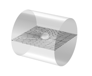
  ${\rm LaCl}_3$ are frequently used in experiments. In addition to the sphere, we consider a cylindrical channel of radius
  $a_c$, length
  $l$ with an uncharged polarizable wall and filled with a corresponding electrolyte solution (cf. figure 1b). The aqueous solution is assumed to have a constant electric permittivity
  $\varepsilon _0\varepsilon _e$, mass density
  $\rho$ and viscosity
  $\mu$. The permittivity of the polarizable solid material is
  $\varepsilon _0\varepsilon _s$, and the permittivity ratio of the polarizable solid and the electrolyte is denoted as
  $\varepsilon _r=\varepsilon _s/\varepsilon _e$. It should be noted that, while we model the solid as a dielectric material, for a very large permittivity ratio and a steady-state scenario we reach equivalence to a conductive material. In both cases (high-permittivity dielectric and conductor), the surface of the material becomes an isopotential surface, and the interior of the material becomes field free.

Figure 1. Schematic representation of the computational domains for (a) the sphere of radius  $a_p$ and (b) the nanochannel of radius
  $a_c$, length
  $l$. The computational domains (two-dimensionally axisymmetric
  $(r,z)$) are enclosed by red dashed lines in both cases. Sufficiently large liquid domains of dimensions
  $r_{p,\infty }$ and
  $r_{c,\infty }$ are considered adjacent to the sphere and channel, respectively. The boundary conditions are indicated in the boxes.
An external electric field of strength  $E_0$ is applied along the positive
  $z$ direction in both scenarios. The electric potential
  $\phi _s$ inside the polarizable solid with no free charge obeys the Laplace equation
 \begin{equation} \boldsymbol{\nabla}\boldsymbol{\cdot}\left(\varepsilon_0\varepsilon_s\boldsymbol{\nabla}\phi_s\right) =0, \end{equation}
whereas the electric potential  $\phi$ inside the liquid domain obeys the Poisson equation
 \begin{equation} \boldsymbol{\nabla}\boldsymbol{\cdot}\left(\varepsilon_0\varepsilon_e\boldsymbol{\nabla}\phi\right)=-\rho_e. \end{equation}
Here,  $\rho _e=F(z_1c_1+z_2c_2)$ denotes the space charge density, with
  $F$ being the Faraday constant and
  $c_i$ and
  $z_i$
$z_i$  $(i=1,2)$ representing the molar ionic concentration and valence of
  $i$th species, respectively. The concentration fields are governed by the Nernst–Planck equation
 \begin{equation} \partial_t c_i + \boldsymbol{\nabla}\boldsymbol{\cdot} \left[ c_i {\boldsymbol{u}} - D_i\boldsymbol{\nabla} c_i - \frac{z_i D_i F}{RT}c_i\boldsymbol{\nabla}\phi \right]= 0, \end{equation}
with  $D_i$
$D_i$  $(i=1,2)$ being the diffusion coefficients of the ions, and
  $R$,
$R$,  $T$ the gas constant and the absolute temperature, respectively. Finally, the velocity field
  $\boldsymbol {u}$ of the liquid is modelled via the continuity equation
 \begin{equation} \boldsymbol{\nabla}\boldsymbol{\cdot} {\boldsymbol{u}} =0, \end{equation}
and the incompressible Navier–Stokes equation with an electrostatic body force
 \begin{equation} \rho\left[\partial_t {\boldsymbol{u}}+( {\boldsymbol{u}}\boldsymbol{\cdot}\boldsymbol{\nabla}) {\boldsymbol{u}}\right]=-\boldsymbol{\nabla} p + \mu\nabla^2{\boldsymbol{u}} -\rho_e\boldsymbol{\nabla}\phi, \end{equation}
with  $p$ representing the pressure field. We numerically solve the governing equations in a two-dimensional axisymmetric model with coordinates
  $(r,z)$ using the finite-element method (see Appendix A for details).
Symmetry boundary conditions for all variables are applied at  $r=0$ in both cases. At the solid–liquid interface, continuity of the electric potential
  $\phi =\phi _s$ and a jump condition for the electric field
  $\varepsilon _0\varepsilon _e\boldsymbol {n}\boldsymbol{\cdot}\boldsymbol {\nabla }\phi =\varepsilon _0\varepsilon _s\boldsymbol {n}\boldsymbol{\cdot}\boldsymbol {\nabla }\phi _s$ apply in the absence of an inherent surface charge density. Also, the no-slip (
 $\boldsymbol {u}=0$) and zero ion flux (
 ${\boldsymbol {n}\boldsymbol{\cdot}[ c_i {\boldsymbol {u}} - D_i\boldsymbol {\nabla } c_i -(z_iD_iF/RT)c_i\boldsymbol {\nabla }\phi ]=0}$) boundary conditions are implemented at the solid–liquid interface. Here,
  $\boldsymbol {n}$ and
  $\boldsymbol {t}$ represent the normal vector and tangent vector at that surface, respectively. Bulk ionic concentrations
  $c_i=c_{i0}$,
  $i=1,2$, and a zero stress
  $\boldsymbol {n}\boldsymbol{\cdot}[ -p\boldsymbol {{I}}+\mu ( \boldsymbol {\nabla } \boldsymbol {u} + \boldsymbol {\nabla }\boldsymbol {u}^T )]=0$ condition are applied in the far field, i.e. either far away from the particle or channel. An electric field of strength
  $E_0$ is applied via the Dirichlet boundary condition
  $\phi =-E_0z$ for the case of the particle, and
  $\phi =E_0l$ at the bottom, as well as
  $\phi =0$ at top of the reservoirs for the case of the channel. The boundary conditions are depicted in figures 1(a) and 1(b).
The bulk concentration of the electrolyte and the strength of the electric field are always considered to be sufficiently low. This allows us to neglect the variation in the fluid properties such as permittivity, viscosity and density due to the redistribution of ions. Moreover, the limited electric field strength translates to negligible effects due to ohmic heating. For this reason, we assume a constant temperature in the entire domain. Thus, temperature-induced variations of the fluid properties can also be ignored.
3. Ion concentration field and velocity field around an uncharged polarizable sphere
We start our discussion by exploring the ion distribution and flow field around an uncharged polarizable sphere, with the origin of the  $(r,z)$ coordinate system attached to its centre. An example would be a metal sphere, which in electrostatics is represented by a medium of infinite dielectric permittivity to ensure that its interior is field free. The flow field around an uncharged polarizable surface is caused by the induced zeta potential, which in turn gives rise to an EDL that represents a space charge distribution (Bazant & Squires Reference Bazant and Squires2004; Squires & Bazant Reference Squires and Bazant2004). Previous studies have revealed a bipolar distribution of the induced zeta potential which vanishes when averaged over the surface (Squires & Bazant Reference Squires and Bazant2006; Yossifon et al. Reference Yossifon, Frankel and Miloh2006; Bazant & Squires Reference Bazant and Squires2010; Bhattacharyya & Majee Reference Bhattacharyya and Majee2017; Feng et al. Reference Feng, Chang, Zhong and Wong2020). In the present study we especially focus on asymmetric electrolytes. We find that, in such a case, the antisymmetry under
  $z \rightarrow -z$ is broken and averaging the zeta potential over the surface gives a non-zero value (cf. figure 3a). However, in spite of that, the net charge on the sphere vanishes. At a fixed bulk concentration
  $c_0=10$ mM, the space charge density and velocity field are shown in figure 2(a–c) for different electrolytes. As the valence of the ions increases, the EDL thickness decreases due to an enhanced attraction between the charges induced at the surface and the charges in the diffuse part of the EDL.

Figure 2. Space charge density  $\rho _e=F(c_1z_1+c_2z_2)$ in the background and streamlines in the foreground around a highly polarizable uncharged spherical particle for three different types of electrolyte (a) KCl, (b)
  ${\rm BaCl}_2$ and (c)
  ${\rm LaCl}_3$ at
  $c_0=10$ mM,
  $\varepsilon _r=10^4$,
  $E_0=10^5\ {\rm V}\ {\rm m}^{-1}$,
  $a_p=100$ nm.
Different from the case of a symmetric electrolyte (such as KCl), the space charge density for  ${\rm BaCl}_2$ and
  ${\rm LaCl}_3$ exhibits an asymmetric distribution in two ways (cf. figure 2a–c). First, the thickness of the EDL that contains a majority of cations (i.e.
  ${\rm Ba}^{+2}$ or
  ${\rm La}^{+3}$) is lower than the EDL thickness in those regions with an excess of anions (
 ${\rm Cl}^-$). Second, the surface areas occupied by induced surface charges of different polarity are not identical. The part of the EDL with a majority of monovalent counterions covers a larger surface compared with the part with a majority of multivalent counterions. The former is attributed to the increased electrostatic attraction of the multivalent counterions compared with monovalent counterions, whereas the second type of asymmetry comes about to preserve the net electroneutrality of the uncharged sphere. The asymmetry of the space charge density results in an asymmetric velocity distribution around the sphere. Figure 2(b,c) shows that the vortex structure around the sphere becomes asymmetric in the case of asymmetric electrolytes. The flow structure is significantly different from the well-known quadrupolar vortices (figure 2a) typically encountered in the vicinity of uncharged spheres (Bazant & Squires Reference Bazant and Squires2004). Importantly, integrating the
  $z$-component of the flow velocity over any plane
  $z={\rm const}.$ yields a zero result in the case of a symmetric electrolyte, whereas for
  ${\rm BaCl}_2$ and
  ${\rm LaCl}_3$ a non-vanishing flow is found. This means that, in the case of charge-asymmetric electrolytes, even an uncharged sphere with homogeneous surface properties has a non-vanishing electrophoretic mobility.
4. Theoretical model
We developed a theoretical model to highlight the key parameters responsible for the emergence of a net ICEO flow. The underlying assumptions are a small Debye length  $(\lambda _D\ll a_p)$, a weak electric field (
 $E_0 a_p\ll k_{{\rm B}}T/e$, where
  $k_{{\rm B}}$ is the Boltzmann constant) and a highly polarizable particle
  $(\epsilon _r\gg 1)$.
4.1. Modified Grahame equation
The relation between surface potential  $(\psi )$ and surface charge density
  $(\sigma )$ for a binary, symmetric electrolyte is given by the Grahame equation as
 \begin{equation} \sigma=\frac{2\varepsilon_0\varepsilon_e\phi_0}{\lambda_D} \sinh{\left(\frac{\psi}{2\phi_0} \right)}, \end{equation}
where  $\lambda _D=\sqrt {\varepsilon _0\varepsilon _e\phi _0 /2c_0F}$ represents the EDL thickness and
  $\phi _0=k_{{\rm B}}T/e$ denotes the thermal potential. Identifying the zeta potential
  $(\zeta )$ with the surface potential, and under the Debye–Hückel approximation, the above relation can be simplified as
 \begin{equation} \sigma=\frac{\varepsilon_0\varepsilon_e\zeta}{\lambda_D}. \end{equation}
Following a similar approach, we can obtain a  $\sigma -\zeta$ relation for a binary electrolyte with arbitrary ionic valencies. The one-dimensional Poisson equation in the wall-normal direction is
 \begin{equation} \partial_x^2 \psi =-F(z_1c_1+z_2c_2), \end{equation}
with the ion concentrations given as
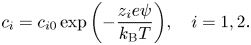 \begin{equation} c_i=c_{i0}\exp{\left( - \frac{z_ie\psi}{k_{{\rm B}}T} \right)},\quad i=1,2. \end{equation}
From that, we obtain the  $\sigma -\zeta$ relation for a binary electrolyte with arbitrary ionic valencies under the Debye–Hückel approximation as
 \begin{equation} \sigma=\sqrt{-\frac{z_1z_2|z_1-z_2|}{2}} \left( \frac{\varepsilon_0\varepsilon_e\zeta}{\lambda_D} \right)\sqrt{ 1- \left(\frac{z_1+z_2}{3}\right)\frac{e\zeta}{k_{{\rm B}}T} }. \end{equation}
The square root term in (4.5) is expanded and approximated by neglecting  $O( ( e\zeta /k_{{\rm B}}T )^3)$ and higher-order terms. This leads to the generalized Grahame equation for asymmetric electrolytes
 \begin{equation} \sigma=\sqrt{-\frac{z_1z_2|z_1-z_2|}{2}} \left( \frac{\varepsilon_0\varepsilon_e\zeta}{\lambda_D} \right)\left[ 1- \left(\frac{z_1+z_2}{6}\right)\frac{e\zeta}{k_{{\rm B}}T} \right]. \end{equation}
The above (4.6) represents the relation between the zeta potential  $(\zeta )$ and the surface charge density
  $(\sigma )$ for a binary electrolyte with arbitrary ionic valencies under the Debye–Hückel approximation. It reduces to (4.2) for a symmetric electrolyte, i.e. for
  $z_1=-z_2$.
4.2. Electrostatic boundary condition at the solid–liquid interface
In the liquid domain, the electric potential  $\phi$ follows the Poisson equation (2.2). Assuming a sufficiently thin EDL, (2.2) can be considered on a locally planar geometry (in wall-normal direction) as follows:
 \begin{equation} \varepsilon_0\varepsilon_e \partial^2_x\phi=-\rho_e. \end{equation}
Here,  $\rho _e$ denotes the space charge density. Integrating (4.7) from the solid–liquid interface to the outer edge of the EDL we obtain
 \begin{equation} \varepsilon_0\varepsilon_e \int_0^{\lambda_D} \partial^2_x\phi \,{{\rm d}\kern0.06em x}=- \int_0^{\lambda_D}\rho_e \,{{\rm d}\kern0.06em x}. \end{equation}
Considering the electroneutrality condition, the right-hand side of (4.8) represents the total number of charges contained in the EDL and can be expressed in terms of the potential drop across the EDL ( $\phi |_{x=\lambda _D}-\phi |_{x=0}$) i.e. the induced
  $\zeta$ potential. This relation is given by (4.6). In line with Zhao & Yang (Reference Zhao and Yang2009), we assume that
  $\boldsymbol {n}\boldsymbol{\cdot}\boldsymbol {\nabla }\phi$ vanishes at the outer edge of the EDL i.e. at
  $x=\lambda _D$. Thus, (4.8) leads to
 \begin{equation} \varepsilon_0\varepsilon_e \boldsymbol{n}\boldsymbol{\cdot}\boldsymbol{\nabla}\phi |_{x=0}=-\sqrt{-\frac{z_1z_2|z_1-z_2|}{2}} \left( \frac{\varepsilon_0\varepsilon_e\zeta}{\lambda_D} \right)\left[ 1- \left(\frac{z_1+z_2}{6}\right)\frac{e\zeta}{k_{{\rm B}}T} \right]. \end{equation}
Utilizing the jump condition for the electric field at the solid–liquid interface  ${\varepsilon _0\varepsilon _e\boldsymbol {n}\boldsymbol{\cdot} \boldsymbol {\nabla }\phi |_{x=0}=\varepsilon _0\varepsilon _s\boldsymbol {n}\boldsymbol{\cdot}\boldsymbol {\nabla }\phi _s|_{x=0}}$, the left-hand side of the above (4.9) can be expressed in terms of
  $\phi _s$. Moreover, considering the induced
  $\zeta =[\phi _s|_{x=0}-\phi |_{x=\lambda _D}]$ and the continuity of the electric potential at the solid–liquid interface, (4.9) can be expressed as
 \begin{equation} \phi_s + \sqrt{ \frac{-2}{z_1z_2|z_1-z_2|}} \left( \frac{\lambda_D \varepsilon_s}{\varepsilon_e} \right) \boldsymbol{n}\boldsymbol{\cdot}\boldsymbol{\nabla}\phi_s = \phi + \left(\frac{z_1+z_2}{6}\right)\frac{(\phi_s-\phi )^2}{k_{{\rm B}}T/e}. \end{equation}
The above (4.10) represents the electrostatic boundary condition at the interface between an uncharged polarizable solid and a binary electrolyte with arbitrary ionic valencies in the thin EDL limit. It reduces to the well-established boundary condition  $[{\phi _s + (\lambda _D \varepsilon _s/\varepsilon _e) \partial _n\phi _s=\phi} ]$ at the solid–liquid interface for a symmetric electrolyte (Yossifon et al. Reference Yossifon, Frankel and Miloh2006).
4.3. Induced zeta potential on the spherical particle
The dimensionless electric potential  $\varPhi _s=\phi _s/\phi _0$,
  $\phi _0=(k_{{\rm B}}T/e)$ inside the spherical particle follows the Laplace equation (2.1). Assuming axisymmetry and using a spherical coordinate system (
 $\varrho,\theta$), it is given by
 \begin{equation} \bar{\nabla}^2\varPhi_s= \frac{\partial}{\partial \varrho}\left( \varrho^2 \frac{\partial \varPhi_s}{\partial \varrho} \right) + \frac{1}{\sin{\theta}} \frac{\partial}{\partial \theta}\left( \sin{\theta} \frac{\partial \varPhi_s}{\partial\theta}\right)=0. \end{equation}
Using the separation of variables technique, the solution of the above (4.11) can be written in the well-known form
 \begin{equation} \varPhi_s(\varrho,\theta)= \sum_{n=0}^\infty \left[ \mathcal{A}_n \varrho^n + \mathcal{B}_n \varrho^{-(n+1)}\right]\mathcal{P}_n(\cos{\theta}). \end{equation}
Here,  $\mathcal {P}_n(\cos {\theta })$ represents the Legendre polynomials. Similarly, under the thin EDL assumption, the non-dimensional electric potential
  $\varPhi$ inside the liquid also obeys the Laplace equation
  $\bar {\nabla }^2\varPhi =0$. Under the approximations made, at steady state the ion flux at the solid–liquid interface only has a contribution from electromigration (Squires & Bazant Reference Squires and Bazant2004). Therefore, demanding a vanishing ion flux into the solid is equivalent to the condition
  $\boldsymbol {n} \boldsymbol{\cdot} \bar {\nabla }\varPhi =0$. Utilizing this condition at the solid–liquid interface, the electric potential is given as (Squires & Bazant Reference Squires and Bazant2004)
 \begin{equation} \varPhi(1,\xi)=-\frac{3\varLambda}{2}\mathcal{P}_1(\xi). \end{equation}
Here,  $\varLambda =E_0a_p/\phi _0$ represents the dimensionless external electric field,
  $a_p$ denotes the radius of the spherical particle and
  $\xi =\cos {\theta }$. We assume
  $\varLambda \ll 1$, i.e. the analysis is performed for sufficiently weak electric fields. Using the above (4.13) we can write the interface boundary condition equation (4.10) in the following non-dimensional form:
 \begin{align} &\varPhi_s(1,\xi) + \alpha
\boldsymbol{n} \boldsymbol{\cdot} \bar{\nabla}
\varPhi_s(1,\xi) - \beta \varPhi_s^2(1,\xi) +
3\beta\varLambda \varPhi_s(1,\xi)\mathcal{P}_1(\xi)\nonumber\\ &\quad=
\frac{3\beta\varLambda^2}{4} \mathcal{P}_0(\xi) -
\frac{3\varLambda}{2}\mathcal{P}_1(\xi) +
\frac{3\beta\varLambda^2}{2}\mathcal{P}_2(\xi).
\end{align}
\begin{align} &\varPhi_s(1,\xi) + \alpha
\boldsymbol{n} \boldsymbol{\cdot} \bar{\nabla}
\varPhi_s(1,\xi) - \beta \varPhi_s^2(1,\xi) +
3\beta\varLambda \varPhi_s(1,\xi)\mathcal{P}_1(\xi)\nonumber\\ &\quad=
\frac{3\beta\varLambda^2}{4} \mathcal{P}_0(\xi) -
\frac{3\varLambda}{2}\mathcal{P}_1(\xi) +
\frac{3\beta\varLambda^2}{2}\mathcal{P}_2(\xi).
\end{align}
Here, the non-dimensional numbers  $\alpha$ and
  $\beta$ are given as
  $\alpha =\sqrt {-2/z_1z_2|z_1-z_2|}(\varepsilon _r/\kappa a_p)$ and
  $\beta =(z_1+z_2)/6$, respectively, with
  $\kappa ^{-1}=\lambda _D$ and
  $\varepsilon _r=\varepsilon _s/\varepsilon _e$. In the present context,
  $\alpha$ becomes
  $\varepsilon _r/\kappa a_p$ and
  $\beta$ vanishes for a binary monovalent electrolyte. Under the assumption of the particle being highly polarizable we have
  $\varPhi _s\ll 1$. Thus, the term proportional to
  $\varPhi _s^2$ on the left-hand side of (4.14) can be neglected. Moreover, the last term on the left-hand side of (4.14) can also be neglected, as
  $\varLambda \ll 1$. Then, the boundary condition at the solid–liquid interface becomes
 \begin{equation} \varPhi_s(1,\xi) + \alpha \boldsymbol{n} \cdot \bar{\nabla} \varPhi_s(1,\xi) = \frac{3\beta\varLambda^2}{4} \mathcal{P}_0(\xi) - \frac{3\varLambda}{2}\mathcal{P}_1(\xi) + \frac{3\beta\varLambda^2}{2}\mathcal{P}_2(\xi). \end{equation}
Solving the Laplace equation (4.11) inside the sphere with the boundary condition (4.15), we obtain the dimensional electric potential ( $\phi _s=\varPhi _s \phi _0$) as
 \begin{align} \phi_s(\varrho,\theta)=\frac{3\beta}{4} \left( \frac{E_0^2a_p^2}{\phi_0} \right) - \frac{3}{2}\left( \frac{E_0\varrho}{1+\alpha}\right)\cos{\theta} + \frac{3\beta}{4}\left( \frac{E_0^2\varrho^2}{\phi_0(1+2\alpha)} \right) \left(3\cos^2{\theta} -1\right). \end{align}
The above (4.16) represents the electric potential inside a highly polarizable  $(\alpha \gg 1)$ uncharged spherical particle immersed in an asymmetric electrolyte, assuming a sufficiently large ion concentration
  $(\lambda _D\ll a_p)$ and a weak electric field
  $(E_0 a_p\ll \phi _0)$. To obtain the induced zeta potential on the particle surface, one needs to compute the difference of the external and internal electric potentials on the surface, i.e.
  ${\zeta (\theta )=[\phi _s-\phi ]_{\varrho =a_p}}$. The result is given by
 \begin{equation} \zeta(\theta)= \frac{3}{2}E_0 a_p\left( \frac{\alpha}{1+\alpha}\right)\cos{\theta} + \left( \frac{z_1+z_2}{8} \right) \frac{E_0^2 a_p^2}{\phi_0}\left( \frac{3\cos^2{\theta}+2\alpha}{1+2\alpha} \right). \end{equation}
Under the assumption of a highly polarizable/conducting particle ( $\alpha \to \infty$), (4.17) is further simplified and yields the induced zeta potential at the particle surface as follows:
 \begin{equation} \zeta(\theta)=\frac{3}{2}E_0 a_p \cos{\theta} + \left(\frac{z_1+z_2}{8}\right) \frac{E_0^2 a_p^2}{(k_{{\rm B}}T/e)}. \end{equation}
Equation (4.18) is valid in the limiting case of an infinite permittivity ratio between particle and liquid. It reduces to the known expression when a symmetric electrolyte is considered (Squires & Bazant Reference Squires and Bazant2004). The second term on the right-hand side breaks the antisymmetry under  $z \rightarrow -z$.
Figure 3(a) depicts the induced zeta potential on the surface of an uncharged conducting spherical particle immersed in a symmetric (KCl) and an asymmetric ( ${\rm LaCl}_3$) electrolyte. It demonstrates that the analytical result (4.18) matches well with the numerical result for a highly polarizable particle. Since numerically it is not possible to account for the limiting case
  $\varepsilon _r \rightarrow \infty$, the simulations were carried out for
  $\varepsilon _r=10^4$. As apparent in figure 3(a), the induced zeta potential obtained for KCl is symmetric with respect to
  $z \rightarrow -z$ and leads to a vanishing average zeta potential i.e.
  $\int _0^{\rm \pi} \zeta _{KCl}(\theta ) \,{\rm d}\theta =0$. By contrast, the induced zeta potential for an asymmetric electrolyte (
 ${\rm LaCl}_3$, in figure 3a) becomes asymmetric and thus results in a non-zero average zeta potential i.e.
  $\int _0^{\rm \pi} \zeta _{{\rm LaCl}_3}(\theta ) \,{\rm d}\theta \neq 0$. Overall, a good agreement between the analytical and the numerical results is observed. It can be intuitively understood that the non-vanishing net axial velocity of the liquid, discussed subsequently, stems from this non-zero net induced zeta potential.
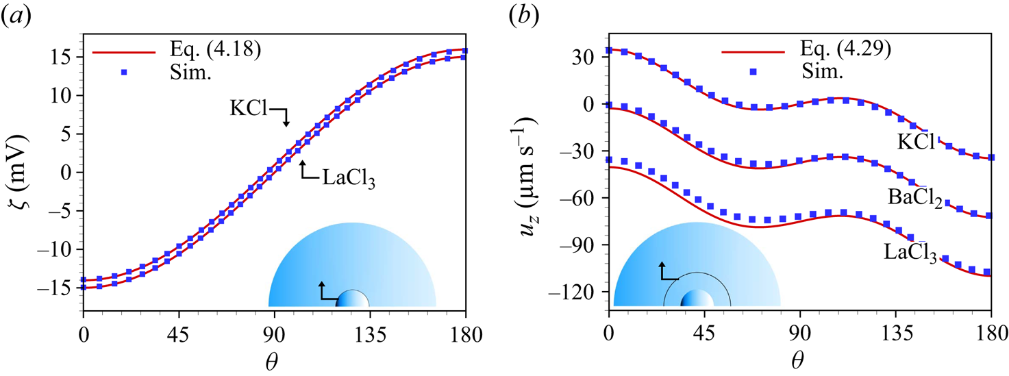
Figure 3. (a) Induced zeta potential on a highly polarizable spherical particle immersed in KCl or  ${\rm LaCl}_3$ solution. (b) Axial velocity of three different electrolyte solutions (KCL,
  ${\rm BaCl}_2, {\rm LaCl}_3$), evaluated on a concentric sphere of radius
  $7 a_p$. The analytical solutions are given by (4.18) for (a) and (4.29) for (b), while the simulation results were obtained for
  $\varepsilon _r=10^4$. The other parameters are
  $c_0=10$ mM,
  $\lambda _D\approx 3$ nm,
  $E_0=10^5\ {\rm V}\ {\rm m}^{-1}$,
  $a_p=100$ nm.
4.4. Net velocity of an uncharged conducting spherical particle immersed in an asymmetric electrolyte
The induced zeta potential of (4.18) consists of two terms, the first one ( $\zeta _1=\frac {3}{2}E_0 a_p \cos {\theta }$) is
  $\theta -$dependent and the second one (
 $\zeta _2=({z_1+z_2}/{8}) {E_0^2 a_p^2}/{\phi _0}$) is constant. Considering that the axial liquid velocity
  $u_z$ can be written as the superposition of the velocities due to varying zeta
  $(u_{1,z})$ and constant zeta
  $(u_{2,z})$, i.e.
  $u_z=u_{1,z}+u_{2,z}$, in the following, again the assumptions of thin EDL, weak electric field and perfectly conducting solid material will be invoked.
At low Reynolds numbers, the momentum equation for an incompressible, Newtonian fluid is given as
 \begin{equation} \boldsymbol{\nabla}p=\mu \nabla^2 \boldsymbol{u}_1, \end{equation}
supplemented by the continuity equation
 \begin{equation} \boldsymbol{\nabla}\boldsymbol{\cdot}\boldsymbol{u}_1=0. \end{equation}
Taking the curl of the momentum equation results in the bi-harmonic equation in terms of the streamfunction as
 \begin{equation} \nabla^4\psi=0. \end{equation}
Here,  $u_{1,\varrho }=({1}/{\varrho ^2 \sin {\theta }})({\partial \psi }/{\partial \theta })$ and
  $u_{1,\theta }=({1}/{\varrho \sin {\theta }})({\partial \psi }/{\partial \varrho })$ are the two velocity components in two-dimensional spherical coordinates (
 $\varrho,\theta$). The streamfunction
  $\psi (\varrho,\theta )$ around a conducting spherical particle of radius
  $a_p$, takes the following form (Taylor Reference Taylor1966):
 \begin{equation} \psi(\varrho,\theta)= \left(\mathcal{C} a_p^4\varrho^{-2} + \mathcal{D} a^2\right) \sin^2{\theta} \cos{\theta}. \end{equation}
Here, the constants  $\mathcal {C},\mathcal {D}$ can be obtained from the corresponding boundary conditions on the particle surface. The velocity components corresponding to (4.22) are
 \begin{equation} \left.\begin{gathered} u_{1,\varrho} = \left(\mathcal{C} a_p^4\varrho^{-2} + \mathcal{D} a^2\right)\left( 2\cos^2{\theta} -\sin^2{\theta}\right) \\ u_{1,\theta} = 2\mathcal{C}a_p^4\varrho^{-4}\sin{\theta}\cos{\theta}. \end{gathered}\right\} \end{equation}
The electric field on the particle surface is given as  $\boldsymbol {E}|_{\varrho =a_p}=(E_\varrho, E_{\theta })|_{\varrho =a_p}=(0,-\frac {3}{2}E_0\sin {\theta })$. We first consider the contribution due to
  $\zeta _1$. The resulting slip velocity
  $(\boldsymbol {u}_{1}^s=-({\varepsilon _0\varepsilon _e\zeta _1}/{\mu })\boldsymbol {E})$ on the particle surface is
  $\boldsymbol {u}_{1}^s|_{\varrho =a_p}=( 0, \frac {9}{8}\mathcal {U}_0 \sin {2\theta } )$, where
  $\mathcal {U}_0=\varepsilon _0\varepsilon _e E_0^2 a_p/\mu$. This translates into the following boundary conditions for the flow field:
 \begin{equation} \left.\begin{gathered} u_{1,\varrho}|_{\varrho=a_p} = 0 \\ u_{1,\theta}|_{\varrho=a_p} = \tfrac{9}{8}\mathcal{U}_0 \sin{2\theta}. \end{gathered}\right\} \end{equation}
Solving (4.22) with these boundary conditions results in the streamfunction
 \begin{equation} \psi(\varrho,\theta)=-\frac{9}{8}\mathcal{U}_0 a_p^2 \left( 1- \frac{a_p^2}{\varrho^2}\right)\sin^2{\theta}\cos{\theta}, \end{equation}
and the corresponding velocity components
 \begin{equation} \left.\begin{gathered} u_{1,\varrho} = \frac{9}{16}\mathcal{U}_0 a_p^2\left( \frac{a_p^2-\varrho^2}{\varrho^4} \right)\left( 1+3\cos{2\theta}\right) \\ u_{1,\theta} = \frac{9}{8}\mathcal{U}_0 \left( \frac{a_p}{\varrho}\right)^4\sin{2\theta}. \end{gathered}\right\} \end{equation}
The velocity components of (4.26) are identical to the total velocity of a symmetric electrolyte around an uncharged conducting spherical particle given in Squires & Bazant (Reference Squires and Bazant2004). After a coordinate transformation, the axial velocity component is obtained as
 \begin{equation} u_{1,z}=\frac{9\mathcal{U}_0}{16}\frac{a_p^2}{\varrho^4}\left[ \left( a_p^2 -\varrho^2\right)\left(1+3 \cos{2\theta} \right)\cos{\theta} - 2a_p^2\sin{2\theta}\sin{\theta} \right] . \end{equation}
The axial velocity component  $u_{2,z}$ due to the constant part of the zeta potential
  $\zeta _2$ is given by the Smoluchowski velocity
 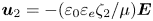 $\boldsymbol {u}_{2}=-({\varepsilon _0\varepsilon _e\zeta _2}/{\mu })\boldsymbol {E}$, i.e.
 \begin{equation} u_{2,z}=-\left(\frac{z_1+z_2}{8}\right)\mathcal{U}_0\frac{E_0 a_p}{\phi_0}, \end{equation}
which, when combined with (4.27), yields the final expression for the total axial velocity field
 \begin{align} u_{z}(\varrho,\theta)&=\frac{9\mathcal{U}_0}{16}\frac{a_p^2}{\varrho^4}\left[ \left( a_p^2 -\varrho^2\right)\left(1+3 \cos{2\theta} \right)\cos{\theta} - 2a_p^2\sin{2\theta}\sin{\theta} \right] \nonumber\\ &\quad -\left(\frac{z_1+z_2}{8}\right)\mathcal{U}_0\frac{E_0 a_p}{\phi_0}. \end{align}
Figure 3(b) shows the axial velocity component along a spherical shell, from the analytical expression and the numerical calculations. As apparent from this figure, the numerical results, obtained at  $c_0=10$ mM and
  $E_0=10^5\ \textrm {V}\ \textrm {m}^{-1}$, match well with the analytical solution. We can observe an asymmetric pattern of the axial velocity for the
  $\textrm {BaCl}_2$ and
  $\textrm {LaCl}_3$ solution, which results in a net axial flow in a direction opposite to the applied electric field. Integrating the axial velocity as given in (4.29) over any concentric sphere, one obtains the average flow velocity, i.e.
  $u_{av}=\int _S u_z \,\textrm {d}S/\int _S \,\textrm {d}S$.
All of the above was evaluated in a frame of reference co-moving with the particle. The resulting electrophoretic particle velocity is just the negative of the average axial flow velocity, i.e.  $u_p=-u_{av} \hat {z}$, which gives
 \begin{equation} u_p=\left(\frac{z_1+z_2}{8}\right)\mathcal{U}_0\frac{E_0 a_p}{\phi_0}. \end{equation}
Substituting the expression of  $\mathcal {U}_0$ one obtains the net particle velocity in the axial direction as
 \begin{equation} u_p=\left( z_1+z_2 \right) \left(\frac{\varepsilon_0\varepsilon_e e}{8 \mu k_{{\rm B}}T}\right)E_0^3 a_p^2 . \end{equation}
Equation (4.31) suggests that an uncharged highly polarizable spherical particle possesses a non-zero electrophoretic mobility if immersed in an asymmetric electrolyte, i.e.  $|z_1|\neq |z_2|$. At the same time, it is evident from (4.31) that the electrophoretic velocity vanishes for a symmetric electrolyte i.e.
  $z_1=-z_2$.
5. Parametric dependencies of the particle velocity
We now discuss the factors influencing the electrophoretic particle velocity in a more general case, i.e. without invoking the assumptions underlying the theoretical model, which, however, means that we need to resort to numerical calculations. Figures 4(a)–4(d) show the electrophoretic velocity as a function of various parameters such as relative permittivity of the particle ( $\varepsilon _r$), the bulk concentration of the electrolyte (
 $c_0$), the radius of the particle (
 $a_p$) and the applied electric field strength (
 $E_0$). The numerical results in figure 4(a,b) exhibit that the electrophoretic velocity increases with
  $\varepsilon _r$ and
  $c_0$. This is because the magnitude of the induced zeta potential increases with the permittivity ratio and with decreasing Debye length. Here, the bulk concentration varies from
  $10^{-2}$ to 10 mM, which corresponds to an approximate EDL thickness of 96 to 3 nm.
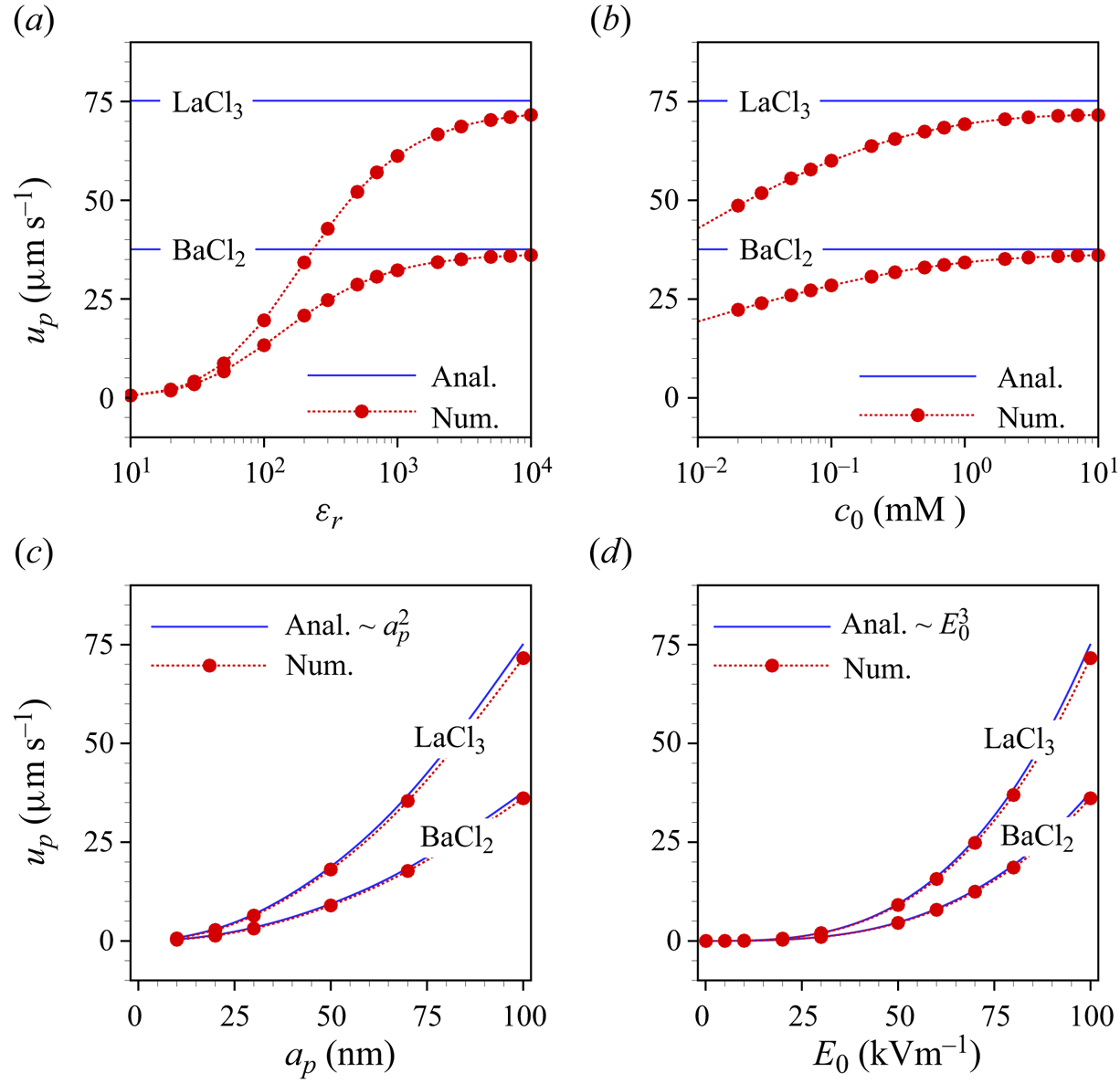
Figure 4. Analytical (solid lines) and numerical (symbols) electrophoretic particle velocity as a function of (a)  $\varepsilon _r$, (b)
  $c_0$, (c)
  $a_p$ and (d)
  $E_0$, for
  $\textrm {BaCl}_2$ and
  $\textrm {LaCl}_3$, respectively. Each case represents variations over a default set of parameters, which is
  $c_0=10$ mM,
  $\varepsilon _r=10^4$,
  $E_0=10^5\ \textrm {V}\ \textrm {m}^{-1}$,
  $a_p=100$ nm.
The analytical result in (4.31), which is obtained assuming a large permittivity ratio and a thin EDL, agrees with the numerical results in both limiting cases (figure 4a,b). Figure 4(c) shows the dependence of the particle velocity on its radius. We find that the velocity increases quadratically with the particle radius, since a larger zeta potential is induced for larger particles. We finally explore the influence of the electric field strength on the electrophoretic velocity in figure 4(d). Both the analytical and simulation results reveal that the velocity is proportional to  $E_0^3$. By contrast, for symmetric electrolytes the local ICEO velocity is proportional to
  $E_0^2$ (Squires & Bazant Reference Squires and Bazant2004). The scaling of the electrophoretic velocity with an odd power of
  $E_0$ is dictated by symmetry arguments, considering that both the velocity and the electric field transform as vectors. In all cases, the electrophoretic velocity obtained for the
  $3:1$ electrolyte is higher than that for the
  $2:1$ electrolyte. In total, the results of figure 4 indicate that, in the case of high permittivity ratios, very significant electrophoretic velocities of uncharged particles are obtained, bearing in mind that a practically relevant value of
  $E_0$ has been chosen. The quadratic scaling of the velocity with the particle radius and the cubic scaling with the electric field strength leave room for even higher velocity values. For example, extrapolation of the curve for
  $\textrm {LaCl}_3$ to a radius of 500 nm using the quadratic scaling yields a velocity of approximately
  $1.75\ \textrm {mm}\ \textrm {s}^{-1}$.
6. Flow inside an uncharged cylindrical channel
We now explore the flow field inside an uncharged cylindrical channel filled with a charge-asymmetric electrolyte solution. It is assumed that the channel walls are composed of a material with high dielectric permittivity. In the case of a metal the structure would represent a floating electrode. Due to the geometric complexity, it is difficult to obtain an analytical solution in this case. Thus, the flow field in the cylindrical channel is solely studied based on the numerical model. Figure 5(a–c) represents the numerically computed space charge density and velocity field inside a cylindrical channel for three different types of salts, KCl,  $\textrm {BaCl}_2$ and
  $\textrm {LaCl}_3$, respectively. As in the case of the spherical particle, the space charge distribution obtained for the asymmetric electrolytes exhibits an asymmetry, with the reflection symmetry along the channel axis broken in terms of both the extension and thickness of the positive/negative space charge regions. This symmetry breaking influences the velocity field and leads to a non-vanishing average velocity (
 $u_{av}$) inside the channel. Here, the average velocity is obtained by integrating the axial velocity component across any cross-section inside the cylindrical channel i.e.
  $u_{av}=\int _0^{a_c} u_z(r,z) 2{\rm \pi} r\,\textrm {d}r/ {\rm \pi}a_c^2$. Subsequently, we study the dependency of
  $u_{av}$ on the problem parameters based on numerical calculations.
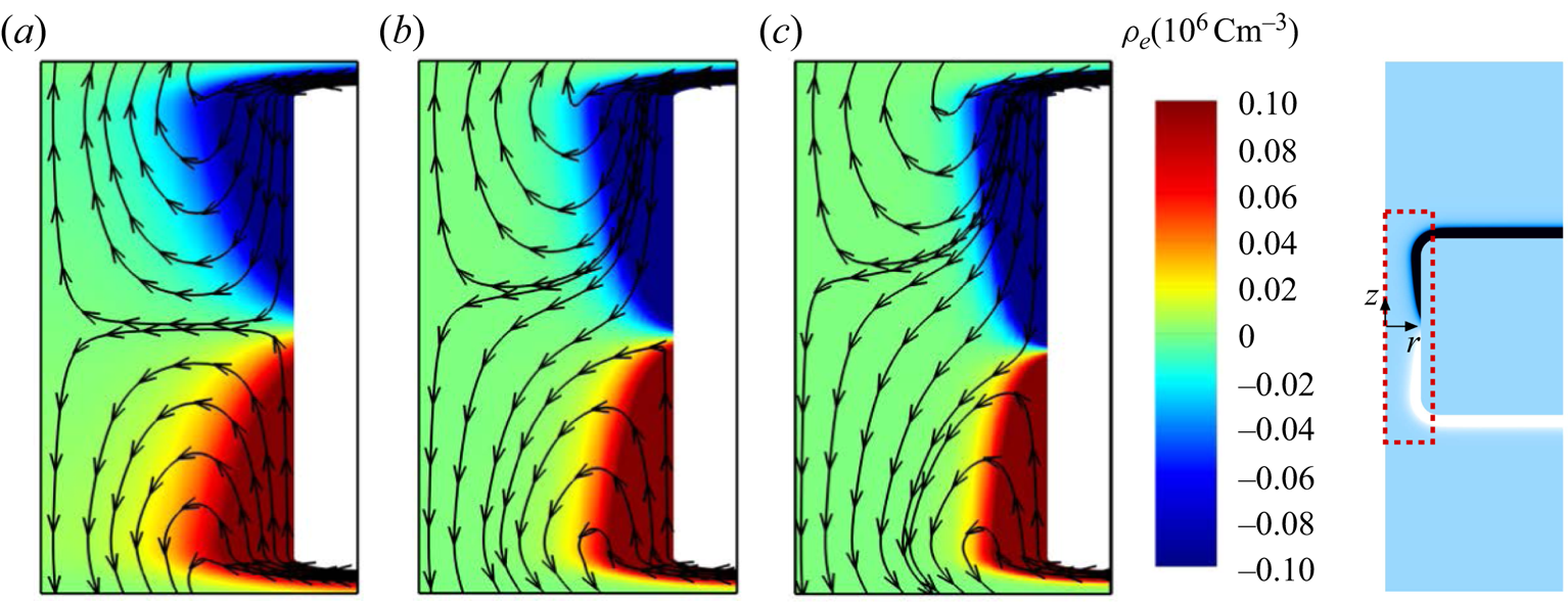
Figure 5. Space charge density and streamlines of the flow field in an uncharged channel for three different types of electrolyte (a) KCl, (b)  $\textrm {BaCl}_2$ and (c)
  $\textrm {LaCl}_3$ at
  $c_0=10$ mM,
  $\varepsilon _r=10^4$,
  $E_0=10^5\ \textrm {V}\ \textrm {m}^{-1}$,
  $a_c=20$ nm,
  $l=0.2\ \mathrm {\mu }\textrm {m}$. In each plot, the boundary on the left represents the symmetry axis. For better visibility, in each plot the horizontal axis was expanded by a factor of 5.24 relative to the vertical one. Results are plotted only in the region highlighted by the red dashed box.
Figure 6(a,b) shows  $|u_{av}|$ as a function of the permittivity ratio
  $(\varepsilon _r)$ and the bulk electrolyte concentration
  $(c_0)$ for
  $\textrm {BaCl}_2$ and
  $\textrm {LaCl}_3$, as well as for two different values of the channel radius,
  $a_c=5,~20$ nm. Here,
  $|u_{av}|$ increases with
  $\varepsilon _r$ and
  $c_0$, which is analogous to the case of the spherical particle. The former occurs because an increase of
  $\varepsilon _r$ goes along with an increasing magnitude of the induced zeta potential. Moreover, the curves in figure 6(a) attain saturation beyond a certain value of
  $\varepsilon _r$. The increase of
  $|u_{av}|$ with
  $c_0$ (cf. figure 6b) can be explained through the fact that the thickness of the EDL decreases with higher concentration and thus results in an enhanced surface potential. We also observe in figures 6(a)–6(e) that the velocity magnitude inside a channel of radius 20 nm is larger than that in a 5 nm channel. The reason is that the electroosmotic velocity attains its maximum value outside the EDL, and a wider cross-section leads to a larger fraction of those regions inside the channel where the velocity is close to its maximum.

Figure 6. Average velocity magnitude in an uncharged nanochannel as a function of (a)  $\varepsilon _r$, (b)
  $c_0$, (c)
  $l$ (low values), (d)
  $l$ (high values), (e)
  $E_0$ (low values) and (f)
  $E_0$ (high values), for
  $\textrm {BaCl}_2$ and
  $\textrm {LaCl}_3$ solutions and two values of the channel radius
  $a_c=5, 20$ nm. The results represent variations over the default parameter set, which is
  $c_0=10$ mM,
  $\varepsilon _r=10^4$,
  $E_0=10^5\ \textrm {V}\ \textrm {m}^{-1}$,
  $l=0.2\ \mathrm {\mu }\textrm {m}$.
The dependence of the average velocity on the channel length is presented in figure 6(c,d). We find that the velocity magnitude is approximately proportional to  $l^2$ and
  $l^{3/2}$ for low and high values of channel length, respectively. The lower range of
  $l$ values roughly corresponds to the regime in which the Debye–Hückel approximation is valid. Beyond that, the induced zeta potential becomes so high that this approximation breaks down. The
  $l^2$ scaling within the Debye–Hückel regime is analogous to the
  $a_p^2$ scaling for the sphere, cf. (4.31). The induced zeta potential obtained as a function of the channel length, plotted in figure 7(a,b), shows that the magnitude of the induced zeta potential increases with increasing channel length, which in turn yields a higher average velocity. In the case of
  $\textrm {LaCl}_3$, the velocity magnitude reaches
  ${\sim }1\ \textrm {mm}\ \textrm {s}^{-1}$ for a
  $1\ \mathrm {\mu }\textrm {m}$ long channel of radius 20 nm. Based on the
  $l^{3/2}$-scaling, a velocity of the order of
  $30\ \textrm {mm}\ \textrm {s}^{-1}$ can be expected for a
  $10\ \mathrm {\mu }\textrm {m}$ long channel, which would be a giant value for such a narrow channel. However, in such a case the induced zeta potential would be very large, which would probably cause ion crowding at the solid surface (Kilic, Bazant & Ajdari Reference Kilic, Bazant and Ajdari2007a,Reference Kilic, Bazant and Ajdarib; Qiao, Tu & Lu Reference Qiao, Tu and Lu2014; Qiao et al. Reference Qiao, Liu, Chen and Lu2016), an effect that is not included in the standard Nernst–Planck model employed here. Therefore, explorations of longer channels containing asymmetric electrolytes are left to future studies.
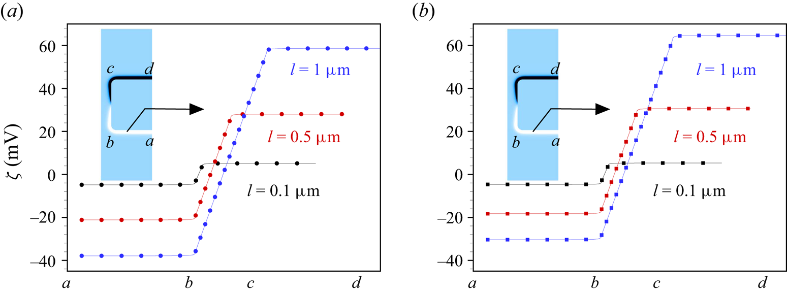
Figure 7. Induced zeta potential along the wall of a highly polarizable cylindrical nanochannel immersed in (a)  $\textrm {BaCl}_2$ and (b)
  $\textrm {LaCl}_3$ solution for different values of the channel length
  $l=0.1,0.5,1\ \mathrm {\mu }\textrm {m}$. The different positions along the solid–liquid interface are indicated on the
  $x$-axis. The other parameters are
  $\varepsilon _r=10^4$,
  $c_0=10$ mM,
  $E_0=10^5\ \textrm {V} \ \textrm {m}^{-1}$ and
  $a_c=100$ nm.
Finally, we study the impact of the electric field strength on the average velocity, cf. figures 6(e) and 6(f). Figure 6(e) shows that the average velocity is proportional to  ${\sim }E_0^3$ for low to moderate values of
  $E_0$. This cubic dependence is equivalent to the particle velocity being proportional to
  $E_0^3$ within the Debye–Hückel limit. However, figure 6(f) indicates that the average velocity no longer obeys the cubic relationship as the electric field becomes stronger, but portrays a proportionality
  ${\sim }E_0^{5/2}$ in that regime. Again, we obtain very significant flow velocities, with maximum values of
  ${\sim }4\ \textrm {mm}\ \textrm {s}^{-1}$ and
  ${\sim }2\ \textrm {mm}\ \textrm {s}^{-1}$ inside nanochannels filled with
  $\textrm {LaCl}_3$ and
  $\textrm {BaCl}_2$ solutions, respectively. Note that even the highest field strength values considered here are still on the lower end of the range of values that are applied in experiments with nanochannels (Gupta et al. Reference Gupta, Liao, Gallego-Perez, Castro and Lee2014; Xiao et al. Reference Xiao, Zhou, Kong, Xie, Li, Zhang, Wen and Jiang2016; Leong et al. Reference Leong, Tsutsui, Yokota and Taniguchi2021; Sornmek et al. Reference Sornmek, Phromyothin, Supadech, Tantisantisom and Boonkoom2022). For the highest experimental values, the
  ${\sim }E_0^{5/2}$ scaling predicts net velocities in excess of metres per second. However, also here, the large induced zeta potentials suggest that the ion crowding will play a role, and beyond a certain threshold, Faradaic reactions on metal surfaces will set in.
7. Concluding remarks
To conclude, we have demonstrated that significant EOFs emerge along surfaces of highly polarizable materials that are exposed to a charge-asymmetric electrolyte solution. We predict that this is a common phenomenon that should be observable even at low ion concentrations and comparatively low imposed electric field strengths. The results were obtained based on the standard framework of the coupled Nernst–Planck, Poisson and Stokes equations. Correspondingly, an uncharged highly polarizable sphere is expected to acquire a very significant electrophoretic mobility, for which our analytical model exhibits the dependencies on the ionic valences, the permittivity ratio between liquid and solid, the electric field strength and on the radius of the sphere. Similarly, a net flow velocity through an uncharged channel in a highly polarizable solid material is predicted. The flow velocity rapidly increases with the length of the channel and the electric field strength, such that a giant electroosmotic pumping is anticipated for scenarios common in experiments. Experimentally examining the giant flow velocities that are predicted using the reported scalings with the channel length and electric field strength should be doable based on the methods and channel structures available to date. Along with that, we suggest extending the mathematical model by taking into account ion crowding effects that are expected to become relevant at high zeta potentials.
Funding
Financial support by the German Research Foundation (DFG), project ID HA 2696/52-1, is gratefully acknowledged.
Declaration of interests
The authors report no conflict of interest.
Appendix A. Numerical simulations
A.1. Grid independence and selection of model parameters
The governing equations are numerically solved by the finite-element method of COMSOL Multiphysics, version 6.1. Quadratic shape functions for the electric potentials  $\phi _s,\phi$, ion concentrations
  $c_i,~i=1,2$, velocity
  $\boldsymbol {u}$ and linear shape function for the pressure
  $p$ are employed. As depicted in figure 8(c,f), the computational domains are discretized using a structured grid. In the case of the channel, to avoid singularities at the corners, the corners are rounded with a radius of 5 nm, and close to the corners a small portion of unstructured grid with triangular cells is added. The numbers of grid cells in the
  $r$ and
  $z$-directions are considered to be proportional to a dummy variable
  $h_p$ (particle configuration) or
  $h_c$ (channel configuration). Thus,
  $h_{i,i=p,c}=2^n, n\in \mathbb {N}$ corresponds to a grid distribution with a refinement factor of
  $2^n,~n\geq 1$, as compared with
  $n=1$. In the present case,
  $h_{i,i=p,c}$ is varied from
  $2^0$ to
  $2^2$.
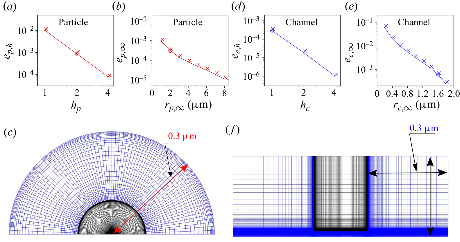
Figure 8. (a,b,d,e) Relative errors obtained from the grid-independence test (a,d) and the finite-size test (b,e) for the particle (a,b) and the channel (d,e). The total number of grid cells in any direction is proportional to  $h_{i,i=p,c}$. The order of convergence obtained is 3.53 for the particle and 3.92 for the channel. (c,f) Grid structures for the particle at
  $h_p=2$,
  $r_{p,\infty }=0.3\ \mathrm {\mu }\textrm {m}$ (c) and the channel at
  $h_c=1$,
  $r_{c,\infty }=0.3\ \mathrm {\mu }\textrm {m}$ (f). For better visibility, relative to figure 5, the channel structure was rotated by
  $90^\circ$. Note that all simulations apart from the grid-independence test were carried out for
  $r_{p,\infty }=2\ \mathrm {\mu }\textrm {m}$ and
  $r_{c,\infty }=1.6\ \mathrm {\mu }\textrm {m}$ (not shown due to poor visibility of the grid structure). The mesh in the liquid and solid domains is presented using blue and black colours, respectively.
The average axial velocity  $u_{av}$ is considered as the quantity for the grid assessment in both cases. It is obtained as
  $u_{av}=\int _S u_z(r,z) \,\textrm {d}S/\int _S \,\textrm {d}S$, where
  $S$ represents either any concentric sphere surrounding the particle or any cross-sections inside the channel. A grid-independent value
  $u_{av,R}$ is derived using Richardson extrapolation. The relative error for a specific value of
  $h_{i,i=p,c}$ is defined as
  $e_{i,h}=(u_{av,h_i}-u_{av,R})/u_{av,R},~i=p,c$. The EDL is of key importance in the considered context and requires a suitable grid resolution to capture the physics. Figure 8(a,d) depicts the relative error
  $e_{i,h},~i=p,c$ for the thinnest EDL considered here, i.e. for a 10 mM
  $\textrm {LaCl}_3$ solution. The relative error is supposed to be smaller than the desired numerical accuracy, which was set to
  $10^{-3}$, and
  $h_p=2$ and
  $h_c=1$ are chosen for the further calculations (cf. figure 8a,d). In addition to the grid-independence study based on the average flow velocity, we have examined the entire flow field at different grid resolutions, represented by
  $h_p=1,2$ and 4. Also this study confirms that the results are virtually grid independent.
Similarly, the size of the reservoirs/liquid domain can affect the flow properties. To rule out significant finite-size effects, the size of the reservoir/liquid domain in both cases is varied systematically, and the relative error  $e_{i,\infty }=(u_{av,h_i}-u_{\infty,h_i})/u_{\infty,h_i}, i=p,c$ is obtained, where
  $u_{\infty,h_p}=u_{av}(r_{p,\infty }=10\ \mathrm {\mu }\textrm {m})$ and
  $u_{\infty,h_c}=u_{av}(r_{c,\infty }=2\ \mathrm {\mu }\textrm {m})$ are considered as approximations for infinitely large reservoirs/domains. Based on the requirement that the relative error is smaller than
  $10^{-3}$, the dimensions are chosen as
  $r_{p,\infty }=2\ \mathrm {\mu }\textrm {m}$ and
  $r_{c,\infty }=1.6\ \mathrm {\mu }\textrm {m}$ (see figure 8b,e) for further calculations. The rest of the model parameters used are presented in table 1.
Table 1. The parameter values used in the present study. If applicable, the parameters refer to a temperature of  $T=298$ K. The values of diffusion coefficients of ionic species are taken from Masliyah & Bhattacharjee (Reference Masliyah and Bhattacharjee2006).
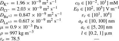
A.2. Validation
In the following, we validate the numerical model for the case of the spherical particle by comparing simulation results with an analytical solution for symmetric salts by Squires & Bazant (Reference Squires and Bazant2004). No analytical solution is available for the governing equations (2.2)–(2.1) in their full form. However, approximate analytical solutions exist when assuming a weak electric field, a thin EDL and a perfectly conducting solid. Thus, to compare with the analytical solution, a 10 mM KCl solution was considered. The analytical solution for the induced zeta potential and the axial velocity under such approximations is given as follows (Squires & Bazant Reference Squires and Bazant2004):
 $$\begin{gather} \zeta(\theta)=\tfrac{3}{2}E_0 a_p\cos{\theta}, \end{gather}$$
 $$\begin{gather}u_z(\varrho,\theta)=\frac{9\mathcal{U}_0}{16}\frac{a_p^2}{\varrho^4}\left[ \left( a_p^2 -\varrho^2\right)\left(1+3 \cos{2\theta} \right)\cos{\theta} - 2a_p^2\sin{2\theta}\sin{\theta} \right]. \end{gather}$$
 Here,  $\mathcal {U}_0=\varepsilon _0\varepsilon _e E_0^2 a_p^2/\mu$ denotes the induced charge electroosmotic slip velocity. It should be noted that the analytical solution was obtained in a two-dimensional spherical coordinate system
  $(\varrho,\theta )$. For the plots of figure 9, the coordinate transformation
  ${\varrho =\sqrt {r^2+z^2}}$,
  $\theta =\arctan {(r/z)}$ was applied. The numerical and the analytical results for the induced zeta potential at the solid–liquid interface and the axial velocity along a concentric sphere are compared in figures 9(a), and 9(b), respectively. While the analytical solution only exists for a perfectly conducting particle, the present numerical results can be obtained for arbitrary values of
  $\varepsilon _r$. Figure 9(a,b) shows that the numerical results match with the analytical results for a sufficiently large value of
  $\varepsilon _r=10^4$. This is in accordance with the fact that in electrostatics, a highly polarizable material (i.e.
  $\varepsilon _r\to \infty$) is equivalent to a perfectly conducting material.

Figure 9. (a) Induced  $\zeta$ potential at the particle–liquid interface and (b) axial velocity
  $u_z$ along a concentric path in the liquid, evaluated at
  $a_p=100$ nm,
  $c_0=10$ mM,
  $\lambda _D\approx 3$ nm,
  $E_0=10^5\ \textrm {V}\ \textrm {m}^{-1}$,
  $\varepsilon _r=10^1,3\times 10^1,10^2,10^4$. The solid lines represent the analytical solutions from (A1), (A2), obtained for a perfectly conducting sphere (Squires & Bazant Reference Squires and Bazant2004), and the symbols indicate the numerical solutions for different permittivities.
Appendix B. Space charge density in the vicinity of the spherical particle
Figure 10(a–c) represents the space charge density adjacent to the uncharged polarizable particle immersed in symmetric/asymmetric electrolytes, i.e. KCl,  $\textrm {BaCl}_2$ and
  $\textrm {LaCl}_3$ solutions. To visualize the asymmetry in the space charge density distribution, the results are obtained at a bulk concentration of 0.01 mM. The black dashed lines in figures 10(a)–10(c) are the curves where the space charge density attains exactly half of its corresponding maximum value. As discussed in the main text, there are two types of asymmetry. First, the EDLs containing a majority of multivalent cations (
 $\textrm {Ba}^{+2}, \textrm {La}^{+3}$) are thinner than the EDLs with a majority of monovalent anions (
 $\textrm {Cl}^-$). Second, the point of zero space charge density is no longer located at the equator. The surface area covered by the EDL with a majority of monovalent counterions (
 $\textrm {Cl}^-$) is larger than the surface area covered by the EDL with a majority of multivalent counterions (
 $\textrm {Ba}^{+2}, \textrm {La}^{+3}$). Both types of asymmetry are clearly visible in figure 10(b,c).

Figure 10. Space charge density  $\rho _e=F(z_1c_1+z_2c_2)$ in the vicinity of an uncharged polarizable particle immersed in different electrolyte solutions ((a) KCl, (b)
  $\textrm {BaCl}_2$ and (c)
  $\textrm {LaCl}_3$), with
  $a_p=100$ nm,
  $c_0=0.01$ mM,
  $E_0=10^5\ \textrm {V}\ \textrm {m}^{-1}$ and
  $\varepsilon _r=10^4$. The dashed lines are the contours where the space charge density attains half of its corresponding maximum value i.e.
  $\rho _{e,max}/2$.


 Open access