


1. Introduction
Neutron stars (NSs) are a natural product of stellar evolution. The main channel of NS formation is related to core-collapse supernovae (SN). The rate of core-collapse SN in the Milky Way now is about 1/50 yrs
 $^{-1}$
(Rozwadowska, Vissani, & Cappellaro, Reference Rozwadowska, Vissani and Cappellaro2021). This number provides a rough estimate
$^{-1}$
(Rozwadowska, Vissani, & Cappellaro, Reference Rozwadowska, Vissani and Cappellaro2021). This number provides a rough estimate
 ${\sim}$
few
${\sim}$
few
 $\times10^8$
NSs in the Galaxy. Today we know about several thousand NS. Mostly, known NSs are radio pulsars (Manchester et al., Reference Manchester, Hobbs, Teoh and Hobbs2005). A few hundred NSs are observed in accreting binary systems (Liu, van Paradijs, & van den Heuvel, Reference Liu, van Paradijs and van den Heuvel2007; Fortin et al., Reference Fortin, García, Bunzel and Chaty2023; Neumann et al., Reference Neumann, Avakyan, Doroshenko and Santangelo2023; Avakyan et al., Reference Avakyan, Neumann, Zainab, Doroshenko, Wilms and Santangelo2023) All other known NSs – magnetars, central compact objects in supernova remnants (CCOs), isolated cooling NSs, etc. – see a review by Popov (Reference Popov2023), – provide less than one hundred objects altogether.
$\times10^8$
NSs in the Galaxy. Today we know about several thousand NS. Mostly, known NSs are radio pulsars (Manchester et al., Reference Manchester, Hobbs, Teoh and Hobbs2005). A few hundred NSs are observed in accreting binary systems (Liu, van Paradijs, & van den Heuvel, Reference Liu, van Paradijs and van den Heuvel2007; Fortin et al., Reference Fortin, García, Bunzel and Chaty2023; Neumann et al., Reference Neumann, Avakyan, Doroshenko and Santangelo2023; Avakyan et al., Reference Avakyan, Neumann, Zainab, Doroshenko, Wilms and Santangelo2023) All other known NSs – magnetars, central compact objects in supernova remnants (CCOs), isolated cooling NSs, etc. – see a review by Popov (Reference Popov2023), – provide less than one hundred objects altogether.
The majority of Galactic NSs are old objects. Their radio pulsar activity (which has a typical duration
 ${\sim}10^7$
yrs, Beskin, Reference Beskin2018) ceased, they are too cold to be observed due to their surface thermal emission, and they do not demonstrate magnetar activity (typical ages of magnetars are
${\sim}10^7$
yrs, Beskin, Reference Beskin2018) ceased, they are too cold to be observed due to their surface thermal emission, and they do not demonstrate magnetar activity (typical ages of magnetars are
 $<10^5$
yrs). Still, there is a way to ‘resurrect’ such a compact object – accretion from the interstellar medium (ISM).
$<10^5$
yrs). Still, there is a way to ‘resurrect’ such a compact object – accretion from the interstellar medium (ISM).
The existence of accreting isolated NSs (AINSs) was proposed more than half a century ago (Ostriker, Rees, & Silk Reference Ostriker, Rees and Silk1970; Shvartsman Reference Shvartsman1971). However, despite many attempts, see, for example, Turner et al. (Reference Turner, Rutledge, Letcavage, Shevchuk and Fox2010) and references therein, not a single robust candidate has ever been proposed. High hopes were placed on ROSAT observations (see, e.g., Treves et al. (Reference Treves, Turolla, Zane and Colpi2000) about AINS studies before the year 2000). Negative results of AINS searches in the ROSAT data were explained by Popov et al. (Reference Popov, Colpi, Treves, Turolla, Lipunov and Prokhorov2000). Due to the large kick velocities that NSs obtain at birth, the onset of accretion is significantly delayed. Under standard at that moment assumptions, Popov et al. (Reference Popov, Colpi, Treves, Turolla, Lipunov and Prokhorov2000) obtained that at most a few percent of old NSs can be observed as accretors, and expected fluxes of most of them are low even for high efficiency of accretion.
The number of AINSs was re-calculated by Boldin & Popov (Reference Boldin and Popov2010) accounting for a significant fraction of highly magnetised NSs and field decay. It was demonstrated that NSs with a high initial magnetic field reach the stage of accretion more rapidly as they spin down faster while the field is high. As only low-velocity NSs in relatively dense regions of the ISM can become accretors within the present Galactic age, in the solar vicinity the fraction of accretors is high: 35–40% (or even twice higher if subsonic propellers are included); high-velocity NSs spend most of their lives high above the Galactic plane in low-density regions.
The physics of accretion at low rates onto magnetised NSs contains many uncertainties. That is why, it was many times analysed numerically (see e.g., Blondin & Raymer (Reference Blondin and Raymer2012); Toropina, Romanova, & Lovelace (Reference Toropina, Romanova and Lovelace2012) and references therein). Still, analytical approaches are very much welcomed, as they allow us to calculate easily the properties of sources with various parameters. A new analytical model of spherical accretion at low rates – so-called settling accretion, – has been proposed not long ago by Shakura et al. (Reference Shakura, Postnov, Kochetkova and Hjalmarsdotter2012). Popov, Postnov, & Shakura (Reference Popov, Postnov and Shakura2015) applied this model to the case of AINSs. These authors concluded that AINS can appear as transient quasi-periodic sources as matter can be accumulated in an envelope around the NS, but the mean luminosity is much lower than predicted by the Bondi formula.
Many uncertainties in the physics of low-rate accretion can be removed if AINSs are finally discovered. Detection of AINSs will be of great value for many reasons. For example, this is the best way to probe the magneto-rotational evolution of NSs on the time scale of about a few Gyrs. In particular, long-term magnetic field decay can be probed in this way.
The behaviour and observational appearance of old NSs also depend on the initial parameters and early evolution. As we mentioned above, the role of kick velocities and initial magnetic fields was studied, already. Initial spin periods never were considered as crucial ingredients because it is typically assumed that they are always short enough –
 ${\lesssim} 1$
s (e.g., Popov & Turolla, Reference Popov and Turolla2012), – to provide a common start for the magneto-rotational evolution. However, the recent discovery of the 76-s radio pulsar PSR J0901-4046 (Caleb et al., Reference Caleb, Heywood, Rajwade, Malenta, Stappers, Barr and Chen2022) challenges this assumption. In addition, two radio sources with periods
${\lesssim} 1$
s (e.g., Popov & Turolla, Reference Popov and Turolla2012), – to provide a common start for the magneto-rotational evolution. However, the recent discovery of the 76-s radio pulsar PSR J0901-4046 (Caleb et al., Reference Caleb, Heywood, Rajwade, Malenta, Stappers, Barr and Chen2022) challenges this assumption. In addition, two radio sources with periods
 ${\sim}1\,000$
s were found: GLEAM-X J1627-52 (Hurley-Walker et al., Reference Hurley-Walker, Zhang, Bahramian, McSweeney, O’Doherty, Hancock, Morgan, Anderson, Heald and Galvin2022) and GPM J1839-10 (Hurley-Walker et al., Reference Hurley-Walker, Rea, McSweeney, Meyers, Lenc, Heywood and Hyman2023). The nature of these objects is not certain (their properties are well summarised for example, by Beniamini et al. (Reference Beniamini, Wadiasingh, Hare, Rajwade, Younes and van der Horst2023)). Still, it is quite plausible that they are young NSs, and the observed periodicity is due to their spin.
${\sim}1\,000$
s were found: GLEAM-X J1627-52 (Hurley-Walker et al., Reference Hurley-Walker, Zhang, Bahramian, McSweeney, O’Doherty, Hancock, Morgan, Anderson, Heald and Galvin2022) and GPM J1839-10 (Hurley-Walker et al., Reference Hurley-Walker, Rea, McSweeney, Meyers, Lenc, Heywood and Hyman2023). The nature of these objects is not certain (their properties are well summarised for example, by Beniamini et al. (Reference Beniamini, Wadiasingh, Hare, Rajwade, Younes and van der Horst2023)). Still, it is quite plausible that they are young NSs, and the observed periodicity is due to their spin.
The origin of long periods is not known, yet. One of the realistic possibilities is related to an episode of fall-back accretion and rapid spin-down of an NS due to interaction with the surrounding matter (Ronchi et al., Reference Ronchi, Rea, Graber and Hurley-Walker2022). Another possibility is related to a rapid spin-down of magnetars due to winds, as suggested by Prasanna et al. (Reference Prasanna, Coleman, Raives and Thompson2022). In this model, the spin period can increase by a factor
 ${\sim} \exp(10)$
during the early cooling stage lasting for
${\sim} \exp(10)$
during the early cooling stage lasting for
 ${\sim} 100$
s. In the model by Ronchi et al. (Reference Ronchi, Rea, Graber and Hurley-Walker2022) long spin periods are achieved on a much longer time scale
${\sim} 100$
s. In the model by Ronchi et al. (Reference Ronchi, Rea, Graber and Hurley-Walker2022) long spin periods are achieved on a much longer time scale
 ${\sim} 10^4$
yrs. Still, it is much shorter than the typical duration of the ejector stage. Thus, we consider spin periods after the phase of a rapid spin-down is over, as initial. If all three long-period radio sources are young NSs then the fraction of such objects can be non-negligible. Then, it is important to consider how long initial spin periods can influence the fate of old isolated NSs.
${\sim} 10^4$
yrs. Still, it is much shorter than the typical duration of the ejector stage. Thus, we consider spin periods after the phase of a rapid spin-down is over, as initial. If all three long-period radio sources are young NSs then the fraction of such objects can be non-negligible. Then, it is important to consider how long initial spin periods can influence the fate of old isolated NSs.
In this paper, we discuss the long-term evolution of NSs, similar to PSR J0901-4046, which have long spin periods already in their youth. For different combinations of parameters, we calculate the age when such NSs can start to accrete from the ISM. In the next section, the general properties of spin evolution of isolated neutron stars (INSs) are reviewed. In Section 3 we describe the specific model of NS magneto-rotational evolution adopted in our work. Then, in Section 4 we present results of the calculations, which are discussed in Section 5. We conclude, summarising our findings, in section 6.
2. Spin evolution of isolated neutron stars
As an INS evolves, it loses rotational energy and interacts with the surrounding material. This results in changing regimes of its behaviour and observational appearance. In this section, we aim to give a brief overview of INS evolutionary stages – ejector, propeller, and accretor – and the transitions between them in terms of critical radii and critical periods.
Let consider the spin evolution of an INS with moment of inertia I, mass M, spin velocity
 $\omega$
and magnetic moment
$\omega$
and magnetic moment
 $\mu$
. The star is moving with the speed
$\mu$
. The star is moving with the speed
 $v_\infty$
through the ISM of number density n and sound velocity
$v_\infty$
through the ISM of number density n and sound velocity
 $c_{\mathrm{s}}$
.
$c_{\mathrm{s}}$
.
The general equation describing the spin evolution of such an NS is the Euler equation:
 \begin{equation} I\frac{\textrm{d}\omega}{\textrm{d}t} = -K,\end{equation}
where K is the spin-down torque acting on the star at a specific stage.
2.1. Ejector
During the ejector evolutionary stage, the ambient matter of the ISM remains far beyond the light cylinder radius
 $R_{\mathrm{l}}$
, which represents the maximum distance at which closed magnetic field lines can exist:
$R_{\mathrm{l}}$
, which represents the maximum distance at which closed magnetic field lines can exist:
 \begin{equation} R_{\mathrm{l}}=\frac{c}{\omega},\end{equation}
where c is the light speed.
At a distance larger than
 $R_{\mathrm{l}}$
, the low-frequency electromagnetic radiation and the flow of relativistic particles sweep the matter out, so the magnetosphere and the surrounding matter do not interact directly. At this stage, the NS slows down due to the ejection of these magnetised winds. The corresponding spin-down torque
$R_{\mathrm{l}}$
, the low-frequency electromagnetic radiation and the flow of relativistic particles sweep the matter out, so the magnetosphere and the surrounding matter do not interact directly. At this stage, the NS slows down due to the ejection of these magnetised winds. The corresponding spin-down torque
 $K_{\mathrm{E}}$
is:
$K_{\mathrm{E}}$
is:
 \begin{equation} K_{\mathrm{E}}=\xi\frac{\mu^2}{R_{\mathrm{l}}^3}.\end{equation}
From the numerical simulation of the plasma-filled magnetosphere, Spitkovsky (Reference Spitkovsky2006) obtained
 \begin{equation} \xi = k_0 + k_1\sin^2\alpha,\end{equation}
where
 $\alpha$
is the angle between the magnetic and spin axes. Later, Philippov, Tchekhovskoy, & Li (Reference Philippov, Tchekhovskoy and Li2014) estimated
$\alpha$
is the angle between the magnetic and spin axes. Later, Philippov, Tchekhovskoy, & Li (Reference Philippov, Tchekhovskoy and Li2014) estimated
 $k_0 \approx 1$
and
$k_0 \approx 1$
and
 $k_1 \approx 1.4$
and showed that their values are weakly dependent on the NS parameters. Note, that often the braking torque at the ejector stage is taken to be smaller. Thus, in our model an NS spins down more effectively and the ejector stage is shorter than in some previous calculations, for example, Boldin & Popov (Reference Boldin and Popov2010).
$k_1 \approx 1.4$
and showed that their values are weakly dependent on the NS parameters. Note, that often the braking torque at the ejector stage is taken to be smaller. Thus, in our model an NS spins down more effectively and the ejector stage is shorter than in some previous calculations, for example, Boldin & Popov (Reference Boldin and Popov2010).
Even though during the ejector stage, the NS magnetosphere does not interact with the surrounding material, the ISM is influenced by the NS presence. The characteristic radius of the gravitational influence of the NS is the gravitational capture radius
 \begin{equation} R_{\mathrm{G}}=\frac{2 G M}{v^2},\end{equation}
where G is the Newton constant and
 $v^2 = v_\infty ^2 + c_{\mathrm{s}}^2$
.
$v^2 = v_\infty ^2 + c_{\mathrm{s}}^2$
.
The amount of interstellar matter that is captured by the NS per unit of time is
 $\dot{{\mathrm{M}}}$
. Following Bondi & Hoyle (Reference Bondi and Hoyle1944), we assume
$\dot{{\mathrm{M}}}$
. Following Bondi & Hoyle (Reference Bondi and Hoyle1944), we assume
 \begin{equation} \dot{{\mathrm{M}}} = \beta\pi R_{\mathrm{G}}^2 n m_{\mathrm{p}} v_{\infty},\end{equation}
where
 $m_{\mathrm{p}}$
is a proton mass. Coefficient
$m_{\mathrm{p}}$
is a proton mass. Coefficient
 $\beta = 1-4$
depending on ratio between
$\beta = 1-4$
depending on ratio between
 $v_{\infty}$
and
$v_{\infty}$
and
 $c_{\mathrm{s}}$
. If
$c_{\mathrm{s}}$
. If
 $c_{\mathrm{s}}$
much smaller than
$c_{\mathrm{s}}$
much smaller than
 $v_{\infty}$
(so that
$v_{\infty}$
(so that
 $v_{\infty} \approx v$
) then
$v_{\infty} \approx v$
) then
 $\beta \approx 1$
.
$\beta \approx 1$
.
Following Shvartsman (Reference Shvartsman1970), the magnetised wind is capable of preventing the matter from being drawn in, if the wind pressure is larger than the pressure of the surrounding matter. We can find the radius
 $R_{\mathrm{Sh}}$
(Shvartsman radius), which is determined by the pressure balance between the wind and the surrounding material:
$R_{\mathrm{Sh}}$
(Shvartsman radius), which is determined by the pressure balance between the wind and the surrounding material:
 \begin{equation} R_{\mathrm{Sh}}=\left( \frac{\xi \mu^2 (GM)^2 \omega^4}{\dot{{\mathrm{M}}} v^5 c^4} \right)^{1/2}.\end{equation}
Here
 $R_{\mathrm{Sh}} > R_{\mathrm{G}}$
since equilibrium can only exist if the Shvartsman radius is larger than the gravitational capture radius (Shvartsman, Reference Shvartsman1970)
$R_{\mathrm{Sh}} > R_{\mathrm{G}}$
since equilibrium can only exist if the Shvartsman radius is larger than the gravitational capture radius (Shvartsman, Reference Shvartsman1970)
While the NS spins down, the Shvartsman radius decreases until it equals either
 $R_{\mathrm{l}}$
or
$R_{\mathrm{l}}$
or
 $R_{\mathrm{G}}$
, depending on which radius is larger. In the latter case, the matter experiences near free-fall conditions before reaching
$R_{\mathrm{G}}$
, depending on which radius is larger. In the latter case, the matter experiences near free-fall conditions before reaching
 $R_{\mathrm{l}}$
. After the matter enters the light cylinder, it begins to interact with the magnetic field. Typically, for INSs with reasonably low velocities
$R_{\mathrm{l}}$
. After the matter enters the light cylinder, it begins to interact with the magnetic field. Typically, for INSs with reasonably low velocities
 $R_{\mathrm{l}} < R_{\mathrm{G}}$
. Hence, the only period of ejector-propeller transition can be written from the condition
$R_{\mathrm{l}} < R_{\mathrm{G}}$
. Hence, the only period of ejector-propeller transition can be written from the condition
 $R_{\mathrm{Sh}} = R_{\mathrm{G}}$
:
$R_{\mathrm{Sh}} = R_{\mathrm{G}}$
:
 \begin{equation}\begin{split} P_{\mathrm{EP}} = \frac{2\pi}{c} \left(\frac{\xi \mu^2}{4 \dot{{\mathrm{M}}} v}\right)^{1/4}. \end{split}\end{equation}
For a ‘standard’ NS with mass
 $1.4{\mathrm{M}_\odot}$
, moment of inertia
$1.4{\mathrm{M}_\odot}$
, moment of inertia
 $10^{45}$
g cm
$10^{45}$
g cm
 $^2$
and radius
$^2$
and radius
 $R = 10$
km this formula can be rewritten as
$R = 10$
km this formula can be rewritten as
 $P_{\mathrm{EP}} \approx 190\,B_{14}^{1/2} v_2^{1/2} n^{-1/4}$
s. Here,
$P_{\mathrm{EP}} \approx 190\,B_{14}^{1/2} v_2^{1/2} n^{-1/4}$
s. Here,
 $B_{14}=B/(10^{14}\,\mathrm{G})$
,
$B_{14}=B/(10^{14}\,\mathrm{G})$
,
 $v_{2}=v/(100$
km s
$v_{2}=v/(100$
km s
 $^{-1})$
,
$^{-1})$
,
 $n = n/(1\,\mathrm{cm}^{-3})$
are assumed along with
$n = n/(1\,\mathrm{cm}^{-3})$
are assumed along with
 $\xi = 2$
(see Section 3). When NS rotation achieves this period, the ejector stage ends and the propeller stage begins. This estimate is based on the assumption that NS is an active radio pulsar, so that it spins down due to both vacuum and wind losses of rotational energy. However, if
$\xi = 2$
(see Section 3). When NS rotation achieves this period, the ejector stage ends and the propeller stage begins. This estimate is based on the assumption that NS is an active radio pulsar, so that it spins down due to both vacuum and wind losses of rotational energy. However, if
 $P_\mathrm{EP} > P_\mathrm{death}$
– a so-called ‘death line’ condition – then one has to consider that after crossing the death line only vacuum losses are relevant. Hence the effective magnetic moment
$P_\mathrm{EP} > P_\mathrm{death}$
– a so-called ‘death line’ condition – then one has to consider that after crossing the death line only vacuum losses are relevant. Hence the effective magnetic moment
 $\mu_\mathrm{vac} = \mu\sin\alpha$
(e.g., Beskin & Eliseeva, Reference Beskin and Eliseeva2005), which leads to
$\mu_\mathrm{vac} = \mu\sin\alpha$
(e.g., Beskin & Eliseeva, Reference Beskin and Eliseeva2005), which leads to
 \begin{equation} P_\mathrm{EP,vac}=P_\mathrm{EP}\sqrt{\sin\alpha} < P_\mathrm{EP}.\end{equation}
However, in the present work we are particularly interested in the fate of the long-period active radio pulsars, so we will omit this correction in the following.
2.2. Propeller
The propeller stage is a necessary step between ejection and accretion. During this evolutionary stage, the interaction of the outer matter with the magnetic field prevents accretion onto the surface of the compact object. The balance between the magnetic field pressure and the pressure of the external matter determines the magnetosphere radius,
 $R_{\mathrm{m}}$
. In the simplest situation, it is equal to the so-called Alfvén radius:
$R_{\mathrm{m}}$
. In the simplest situation, it is equal to the so-called Alfvén radius:
 \begin{equation} R_A = \left( \frac{ \mu^2}{8 \dot{{\mathrm{M}}} \sqrt{2GM}} \right)^{2/7}.\end{equation}
A more detailed analysis of various situations can result in a different definition of
 $R_{\mathrm{m}}$
. For example, according to Davies & Pringle (Reference Davies and Pringle1981),
$R_{\mathrm{m}}$
. For example, according to Davies & Pringle (Reference Davies and Pringle1981),
 $R_{\mathrm{m}}$
slightly exceeds the Alfvén radius due to the existence of an envelope consisting of the heated gravitationally captured material. In this case,
$R_{\mathrm{m}}$
slightly exceeds the Alfvén radius due to the existence of an envelope consisting of the heated gravitationally captured material. In this case,
 $R_{\mathrm{m}}$
represents the radius of the inner boundary of the envelope and can be written as follows:
$R_{\mathrm{m}}$
represents the radius of the inner boundary of the envelope and can be written as follows:
 \begin{equation} R_{\mathrm{m}} = R_A \left (\dfrac{R_{\mathrm{G}}}{R_A} \right)^{2/9}.\end{equation}
Since the magnetic field, which rotates rigidly with the NS, cannot exist outside of the light cylinder, we bound
 $R_{\mathrm{m}}$
from above by the value of
$R_{\mathrm{m}}$
from above by the value of
 $R_{\mathrm{l}}$
.
$R_{\mathrm{l}}$
.
In addition to
 $R_{\mathrm{m}}$
, we note the other important critical radius – the corotation radius
$R_{\mathrm{m}}$
, we note the other important critical radius – the corotation radius
 $R_{\mathrm{c}}$
at which the material can experience an equilibrium between gravitational attraction and centrifugal inertial force:
$R_{\mathrm{c}}$
at which the material can experience an equilibrium between gravitational attraction and centrifugal inertial force:
 \begin{equation} R_{\mathrm{c}} = \left( \frac{GM}{\omega^2} \right)^{1/3}.\end{equation}
During the propeller stage, a rapidly rotating magnetosphere prevents the material from going further than
 $R_{\mathrm{m}}$
. If the material remains at a radius larger than
$R_{\mathrm{m}}$
. If the material remains at a radius larger than
 $R_{\mathrm{c}}$
it cannot fall onto the NS because the centrifugal inertial force overrides the gravitational attraction. Therefore, we consider the propeller stage to exist as long as
$R_{\mathrm{c}}$
it cannot fall onto the NS because the centrifugal inertial force overrides the gravitational attraction. Therefore, we consider the propeller stage to exist as long as
 $R_{\mathrm{m}} > R_{\mathrm{c}}$
.
$R_{\mathrm{m}} > R_{\mathrm{c}}$
.
During the propeller stage, the rotational energy is dissipated at the inner boundary of an atmosphere. Then it is convected up and lost through the outer boundary.
There are a number of ways to describe the NS deceleration at the propeller stage. Below we list some of the possible models proposed for the braking torque
 $K_{\mathrm{P}}$
at this sage, starting with the one with the highest energy losses and ending with the one with the lowest.
$K_{\mathrm{P}}$
at this sage, starting with the one with the highest energy losses and ending with the one with the lowest.
-
(A) Shakura (Reference Shakura1975). In this model, the external matter is considered to be thrown away at a speed close to the rotational speed at the magnetospheric boundary
 $\omega R_{\mathrm{m}}$
. So, the torque
$K_{\mathrm{P}}$
can be written as:(13)where
\begin{equation} K_{\mathrm{P}}=\dot{{\mathrm{M}}} \omega R_{\mathrm{m}}^2 = \frac{1}{8\sqrt{2}}r_{\mathrm{c}}^{-3/2}r_{\mathrm{m}}^{1/2}\frac{\mu^2}{R_{\mathrm{m}}^3},\end{equation}
$r_{\mathrm{c}} = R_{\mathrm{c}}/R_{\mathrm{G}}$
and
$r_{\mathrm{m}} = R_{\mathrm{m}}/R_{\mathrm{G}}$
are dimensionless radii.
$\omega R_{\mathrm{m}}$
. So, the torque
$K_{\mathrm{P}}$
can be written as:(13)where
\begin{equation} K_{\mathrm{P}}=\dot{{\mathrm{M}}} \omega R_{\mathrm{m}}^2 = \frac{1}{8\sqrt{2}}r_{\mathrm{c}}^{-3/2}r_{\mathrm{m}}^{1/2}\frac{\mu^2}{R_{\mathrm{m}}^3},\end{equation}
$r_{\mathrm{c}} = R_{\mathrm{c}}/R_{\mathrm{G}}$
and
$r_{\mathrm{m}} = R_{\mathrm{m}}/R_{\mathrm{G}}$
are dimensionless radii.
-
(B) Davidson & Ostriker (Reference Davidson and Ostriker1973). Here, it is assumed that the material carries away the angular momentum at the free fall velocity
$v_{\mathrm{ff}} = \sqrt{2GM/R_{\mathrm{m}}}$
, hence (14)
\begin{equation} K_{\mathrm{P}} = \dot{{\mathrm{M}}} \sqrt{2GMR_{\mathrm{m}}} = \frac{1}{8} r_{\mathrm{m}}^{-1} \frac{\mu^2}{R_{\mathrm{m}}^3}.\end{equation}
-
(C) Illarionov & Sunyaev (Reference Illarionov and Sunyaev1975). Within this model, the assumed spin-down law is
$I \omega \dot{\omega} = - \dot{{\mathrm{M}}} v_{\mathrm{ff}}^2 / 2 = - GM\dot{{\mathrm{M}}} /R_{\mathrm{m}}$
and the corresponding braking torque is equal to(15)
\begin{equation} K_{\mathrm{P}} = \frac{GM\dot{{\mathrm{M}}}}{\omega R_{\mathrm{m}}} = \frac{1}{8\sqrt{2}}r_{\mathrm{c}}^{3/2}r_{\mathrm{m}}^{-5/2}\frac{\mu^2}{R_{\mathrm{m}}^3}.\end{equation}
-
(D) The supersonic propeller considered by Davies & Pringle (Reference Davies, Fabian and Pringle1979) and Davies & Pringle (Reference Davies and Pringle1981). In this approach, the rotational losses are considered to be constant
$I \omega \dot{\omega} = - \dot{{\mathrm{M}}} v^2 / 2$
, where v contains spatial velocity
$v_{\infty}$
and the acoustic speed
$c_{\mathrm{s}}$
:
$v = \sqrt{v_{\infty}^2 + c_{\mathrm{s}}^2}$
. From this, we can obtain the braking torque: (16)
\begin{equation} K_{\mathrm{P}}= \frac{1}{8\sqrt{2}} r_{\mathrm{c}}^{3/2} r_{\mathrm{m}}^{-3/2}\frac{\mu^2}{R_{\mathrm{m}}^3}.\end{equation}


Once the material reaches a radius smaller than the corotation radius, the centrifugal barrier will no longer prevent it from falling onto the NS. The corresponding transition period can be then calculated from the condition
 $R_{\mathrm{c}} = R_{\mathrm{m}}$
as
$R_{\mathrm{c}} = R_{\mathrm{m}}$
as
 \begin{equation} P_{\mathrm{PA}} = \pi \left(\frac{\mu^2 \sqrt{2}}{GM\dot{{\mathrm{M}}}v^2}\right)^{1/3}.\end{equation}
Using the same parameters of a ‘standard’ NS this formula can be written in a way similar to
 $P_{\mathrm{EP}}$
as
$P_{\mathrm{EP}}$
as
 $P_{\mathrm{PA}} = 3 \times 10^5 B_{14}^{2/3} v_2^{1/3} n^{-1/3}$
s. If the period of the NS exceeds
$P_{\mathrm{PA}} = 3 \times 10^5 B_{14}^{2/3} v_2^{1/3} n^{-1/3}$
s. If the period of the NS exceeds
 $P_{\mathrm{PA}}$
, we consider the NS to change the stage from propeller to accretor.
$P_{\mathrm{PA}}$
, we consider the NS to change the stage from propeller to accretor.
2.3. Accretor
Since accretion starts, several different regimes can be realised depending on circumstances. Following Shakura et al. (Reference Shakura, Postnov, Kochetkova and Hjalmarsdotter2012) we distinguish supersonic (i.e., standard, Bondi or Bondi–Hoyle–Littleton) accretion and subsonic settling accretion.
The first regime is spherical (or cylindrical) accretion of free-falling matter with an accretion rate
 $\dot{{\mathrm{M}}}$
. The most important spatial scale here is the corotation radius
$\dot{{\mathrm{M}}}$
. The most important spatial scale here is the corotation radius
 $R_c$
(see e.g., the derivation of the spin-down torque by Lipunov Reference Lipunov1992). So, neglecting angular momentum accreted from ISM, the spin-down law is
$R_c$
(see e.g., the derivation of the spin-down torque by Lipunov Reference Lipunov1992). So, neglecting angular momentum accreted from ISM, the spin-down law is
 $I \dot{\omega} = -K_{\mathrm{A}}$
, where the angular momentum
$I \dot{\omega} = -K_{\mathrm{A}}$
, where the angular momentum
 $K_{\mathrm{A}}$
can be expressed as follows:
$K_{\mathrm{A}}$
can be expressed as follows:
 \begin{equation} K_{\mathrm{A}}=\zeta\frac{\mu^2}{R_{\mathrm{c}}^3}.\end{equation}
Here
 $\zeta$
is a dimensionless coefficient of the order of unity. It is usually assumed to be
$\zeta$
is a dimensionless coefficient of the order of unity. It is usually assumed to be
 $\zeta \sim 1/3$
(Lipunov, Reference Lipunov1992).
$\zeta \sim 1/3$
(Lipunov, Reference Lipunov1992).
However, the Bondi accretion only occurs if the surrounding material is effectively cooled. A more correct description of the accretion regime realised in our case is the subsonic settling accretion. It is characterised by the existence of a quasi-static atmosphere extending from
 $R_{\mathrm{m}}$
to
$R_{\mathrm{m}}$
to
 $R_{\mathrm{G}}$
. This heated plasma surrounding the NS cools due to convective motions and bremsstrahlung radiation. Thus the characteristic cooling time
$R_{\mathrm{G}}$
. This heated plasma surrounding the NS cools due to convective motions and bremsstrahlung radiation. Thus the characteristic cooling time
 $t_{\mathrm{cool}}$
is significantly longer than the free-fall time
$t_{\mathrm{cool}}$
is significantly longer than the free-fall time
 $t_{\mathrm{ff}}$
. This prevents standard accretion with an accretion rate of
$t_{\mathrm{ff}}$
. This prevents standard accretion with an accretion rate of
 $\dot{{\mathrm{M}}}$
defined by Equation (6).
$\dot{{\mathrm{M}}}$
defined by Equation (6).
As it is shown by Popov, Postnov, & Shakura (Reference Popov, Postnov and Shakura2015), at the settling accretion phase the spin-down torque
 $K_{\mathrm{SA}}$
is slightly different from Equation (18). Namely:
$K_{\mathrm{SA}}$
is slightly different from Equation (18). Namely:
 \begin{equation} K_{\mathrm{SA}} = 8 \dot{{\mathrm{M}}} \omega R_{\mathrm{m}}^2 = \frac{1}{\sqrt{2}}r_c^{3/2}r_m^{-5/2}\frac{\mu^2}{R_{\mathrm{c}}^3},\end{equation}
which coincides with the propeller spin-down torque up to a factor of 8, but here the magnetosphere radius is different from Equation (11), see Popov, Postnov, & Shakura (Reference Popov, Postnov and Shakura2015).
According to Shakura et al. (Reference Shakura, Postnov and Kochetkova2015), the matter in the envelope slowly flows towards the NS with an average velocity
 $u = (t_{\mathrm{ff}} / t_{\mathrm{cool}})^{1/3} v_{\mathrm{ff}}$
, where
$u = (t_{\mathrm{ff}} / t_{\mathrm{cool}})^{1/3} v_{\mathrm{ff}}$
, where
 $v_{\mathrm{ff}}$
is a free-fall velocity. So the maximum possible accretion rate is
$v_{\mathrm{ff}}$
is a free-fall velocity. So the maximum possible accretion rate is
 $\dot{{\mathrm{M}}}_{\mathrm{SA}} \sim (t_{\mathrm{ff}} / t_{\mathrm{cool}})^{1/3} \dot{{\mathrm{M}}}$
. Since
$\dot{{\mathrm{M}}}_{\mathrm{SA}} \sim (t_{\mathrm{ff}} / t_{\mathrm{cool}})^{1/3} \dot{{\mathrm{M}}}$
. Since
 $\dot{{\mathrm{M}}}_{\mathrm{SA}} \ll \dot{{\mathrm{M}}}$
, the X-ray luminosity of potential observable sources could be a few orders of magnitude lower than standard estimates, which take
$\dot{{\mathrm{M}}}_{\mathrm{SA}} \ll \dot{{\mathrm{M}}}$
, the X-ray luminosity of potential observable sources could be a few orders of magnitude lower than standard estimates, which take
 $\dot{{\mathrm{M}}}$
to be an accretion rate.
$\dot{{\mathrm{M}}}$
to be an accretion rate.
Considering the settling accretion regime, Shakura et al. (Reference Shakura, Postnov, Kochetkova and Hjalmarsdotter2012) have shown that the hot envelope surrounding the NS can be also effectively cooled by the Compton process. However, there is a critical value of the X-ray luminosity at which the Compton cooling time becomes equal to the free-fall time. This condition corresponds to
 $\dot{{\mathrm{M}}} \sim 10^{16}$
g s
$\dot{{\mathrm{M}}} \sim 10^{16}$
g s
 $^{-1}$
. This accretion rate is much larger than the possible accretion rate from the ISM. So it can be assumed that the heated material cools only due to bremsstrahlung radiation and the settling accretion regime is established.
$^{-1}$
. This accretion rate is much larger than the possible accretion rate from the ISM. So it can be assumed that the heated material cools only due to bremsstrahlung radiation and the settling accretion regime is established.
On the other hand, Prokhorov, Popov, & Khoperskov (Reference Prokhorov, Popov and Khoperskov2002) have considered the late stages of the Bondi accretion. It is shown that during the standard accretor stage the evolution of the NS period can be influenced by the turbulent angular momentum from the ISM, since the ISM material directly interacts with the magnetosphere. It can both accelerate and decelerate rotation of the NS. The influence of turbulence starts to be important when the NS spins down to the period
 $P_{\mathrm{cr}}$
:
$P_{\mathrm{cr}}$
:
 \begin{equation} P_{\mathrm{cr}} = \frac{2\pi \mu \sqrt{\zeta}}{\sqrt{GM\dot{{\mathrm{M}}}j}},\end{equation}
where specific angular momentum j can be expressed through the characteristic turbulent velocity
 $v_t\simeq 10\,\mathrm{km}\,\mathrm{s}^{-1}$
at the scale
$v_t\simeq 10\,\mathrm{km}\,\mathrm{s}^{-1}$
at the scale
 $R_t\simeq2\times10^{20}$
cm:
$R_t\simeq2\times10^{20}$
cm:
 $j = v_t R_t^{-1/3} R_{\mathrm{G}}^{4/3}$
.
$j = v_t R_t^{-1/3} R_{\mathrm{G}}^{4/3}$
.
 $P_{\mathrm{cr}}$
is defined by
$P_{\mathrm{cr}}$
is defined by
 $K_{\mathrm{A}}=j \dot{{\mathrm{M}}}$
.
$K_{\mathrm{A}}=j \dot{{\mathrm{M}}}$
.
If j exceeds the Keplerian moment at the magnetosphere radius
 $j_K = \sqrt{GMR_{\mathrm{m}}}$
, the disc is formed and the angular momentum in Equation (20) is assumed to be
$j_K = \sqrt{GMR_{\mathrm{m}}}$
, the disc is formed and the angular momentum in Equation (20) is assumed to be
 $j_K$
instead of j. However, the turbulent angular momentum of the ISM for our parameters
$j_K$
instead of j. However, the turbulent angular momentum of the ISM for our parameters
 $j < j_K$
, so we can rewrite Equation (20) in a form
$j < j_K$
, so we can rewrite Equation (20) in a form
 $P_{\mathrm{cr}} = 10^7 B_{14}v_2^{17/6}n^{-1/2}$
s.
$P_{\mathrm{cr}} = 10^7 B_{14}v_2^{17/6}n^{-1/2}$
s.
When
 $P \sim P_{\mathrm{cr}}$
the two processes become comparable. For the periods
$P \sim P_{\mathrm{cr}}$
the two processes become comparable. For the periods
 $P \gtrsim P_{\mathrm{cr}}$
the NS period is significantly affected by the turbulence during the deceleration.
$P \gtrsim P_{\mathrm{cr}}$
the NS period is significantly affected by the turbulence during the deceleration.
According to the consideration of the further influence of the turbulent angular momentum on the deceleration of the NS, conducted by Popov et al. (Reference Popov, Prokhorov, Khoperskov and Lipunov2001), the NS reaches ‘spin equilibrium’. The period evolution begins to be completely determined by the turbulent forces. It fluctuates around the turbulent period:
 \begin{equation} P_{\mathrm{turb}} = 8 \times 10^9 B_{14}^{2/3} v_2^{43/9} n^{-2/3}\,\mathrm{s}\end{equation}
After reaching the turbulent period the NS can both accelerate and decelerate with a characteristic timescale
 ${\sim} R_{\mathrm{G}} / v$
.
${\sim} R_{\mathrm{G}} / v$
.
3. Model
In our work we focus on the modelling P(t) curves and deriving the moments of time when an NS starts to accrete:
 $t=t_{\mathrm{PA}}$
(when
$t=t_{\mathrm{PA}}$
(when
 $P=P_{\mathrm{PA}}$
), enters the turbulent regime:
$P=P_{\mathrm{PA}}$
), enters the turbulent regime:
 $t = t_{\mathrm{cr}}$
(when
$t = t_{\mathrm{cr}}$
(when
 $P=P_{\mathrm{cr}}$
), and reaches the equilibrium:
$P=P_{\mathrm{cr}}$
), and reaches the equilibrium:
 $t=t_{\mathrm{turb}}$
at the period
$t=t_{\mathrm{turb}}$
at the period
 $P_{\mathrm{turb}}$
.
$P_{\mathrm{turb}}$
.
We consider the spin period evolution of an INS with a given initial period
 $P_0$
, initial equatorial magnetic field
$P_0$
, initial equatorial magnetic field
 $B_0$
, and velocity
$B_0$
, and velocity
 $v_\infty$
through the ISM of number density n. Within the calculations we assume
$v_\infty$
through the ISM of number density n. Within the calculations we assume
 $P_0 = 100$
s;
$P_0 = 100$
s;
 $B_0 = 10^{11}$
,
$B_0 = 10^{11}$
,
 $10^{12}, 10^{13}$
or
$10^{12}, 10^{13}$
or
 $10^{14}$
G;
$10^{14}$
G;
 $v_\infty = 30$
or 100 km s
$v_\infty = 30$
or 100 km s
 $^{-1}$
and
$^{-1}$
and
 $n = 0.3$
cm
$n = 0.3$
cm
 $^{-3}$
. Also we try two models of propeller spin-down torque (see the text below) and three models of the magnetic field decay (see Section 3.1). Finally, we assume
$^{-3}$
. Also we try two models of propeller spin-down torque (see the text below) and three models of the magnetic field decay (see Section 3.1). Finally, we assume
 $v_\infty \gg c_{\mathrm{s}}$
, since sound velocity in the ISM
$v_\infty \gg c_{\mathrm{s}}$
, since sound velocity in the ISM
 $c_\mathrm{s} \sim \sqrt{kT/m_\mathrm{p}} \sim 10$
km s
$c_\mathrm{s} \sim \sqrt{kT/m_\mathrm{p}} \sim 10$
km s
 $^{-1}$
for
$^{-1}$
for
 $T \sim 10^4$
K (Klessen & Glover, Reference Klessen, Glover, Revaz, Jablonka, Teyssier and Mayer2016). So, in our calculations
$T \sim 10^4$
K (Klessen & Glover, Reference Klessen, Glover, Revaz, Jablonka, Teyssier and Mayer2016). So, in our calculations
 $v = \sqrt{v_\infty^2 + c_{\mathrm{s}}^2} \approx v_\infty$
.
$v = \sqrt{v_\infty^2 + c_{\mathrm{s}}^2} \approx v_\infty$
.
While the NS spins down, it changes its evolutionary stages. To determine the initial evolutionary stage, the value of
 $P_0$
compares to transition periods of between ejector and propeller
$P_0$
compares to transition periods of between ejector and propeller
 $P_{\mathrm{EP}}$
(Equation 8) and propeller-accretor
$P_{\mathrm{EP}}$
(Equation 8) and propeller-accretor
 $P_{\mathrm{PA}}$
(Equation 17).
$P_{\mathrm{PA}}$
(Equation 17).
At each stage we adopt the spin-down law in the from:
 \begin{equation} \frac{\textrm{d}P}{\textrm{d}t}=\frac{P^2}{2\pi I} K,\end{equation}
where the spin-down torque K is
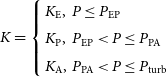 \begin{align*} K = \left\{ \begin {array} {ll} \displaystyle K_{\mathrm{E}}, & P \le P_{\mathrm{EP}} \\ \displaystyle K_{\mathrm{P}}, & P_{\mathrm{EP}} < P \le P_{\mathrm{PA}} \\ K_{\mathrm{A}}, & P_{\mathrm{PA}} < P \le P_{\mathrm{turb}} \\ \end {array} \right.\end{align*}
The particular form of a spin-down torque depends on an evolutionary stage:
-
Ejector. For the ejector stage we take
$K_{\mathrm{E}}$
in a form of Equation (3). In our paper, we consider NSs with long periods
$\gtrsim 100$
s and relatively low velocities
$v \lesssim 100$
km s
$^{-1}$
. For periods and magnetic field values necessary for those NS to be ejectors (>
$10^{13}$
G) the magnetic alignment timescale is longer than the Galaxy lifetime. Therefore we neglect the change in the angle
$\alpha$
over time. Assuming a uniform distribution of newborn NSs over angles we use the mean value of
$\langle \sin^2\alpha \rangle = 2/3$
. So, the factor
$\xi = k_0 + k_1\sin^2\alpha \approx 1.93$
and we take
$\xi = 2$
exactly. -
Propeller. Hereafter we consider only two variants of
$K_{\mathrm{P}}$
: case A (Equation 13) and case B (Equation 14). We do not use C and D models, since the rotational losses in cases C and D can be smaller than the pulsar losses. This contradicts the conclusions by Lipunov & Popov (Reference Lipunov and Popov1995) who demonstrated that spin-down at the ejector stage might be less efficient that at the propeller stage. -
Accretor. We assume the accretion to be standard and use the spin-down torque
$K_{\mathrm{A}}$
in a form of Equation (18) until the equilibrium is reached (
$P = P_{\mathrm{turb}}$
).


After adding the initial condition
 $P(t_0) = P_0$
the initial value problem is numerically solved until the time limit is reached or the period is equal to the transition period (for the ejector and propeller stages this period is respectively
$P(t_0) = P_0$
the initial value problem is numerically solved until the time limit is reached or the period is equal to the transition period (for the ejector and propeller stages this period is respectively
 $P_{\mathrm{EP}}$
and
$P_{\mathrm{EP}}$
and
 $P_{\mathrm{PA}}$
). In the latter case, the new initial value problem is solved. It contains the spin-down law according to a new evolutionary stage and the initial condition in a form
$P_{\mathrm{PA}}$
). In the latter case, the new initial value problem is solved. It contains the spin-down law according to a new evolutionary stage and the initial condition in a form
 $P(t_1) = P_1$
, where
$P(t_1) = P_1$
, where
 $P_1$
is the corresponding transition period, which was reached during previous calculations, and
$P_1$
is the corresponding transition period, which was reached during previous calculations, and
 $t_1$
is the time of the transition to this stage.
$t_1$
is the time of the transition to this stage.
At the accretor stage, we are also interested in the moment of NS entry into the turbulent regime
 $t_{\mathrm{cr}}$
for
$t_{\mathrm{cr}}$
for
 $P=P_{\mathrm{cr}}$
(
$P=P_{\mathrm{cr}}$
(
 $P_{\mathrm{cr}}$
is described by Equation 20), where the turbulence can significantly influence the NS period. For
$P_{\mathrm{cr}}$
is described by Equation 20), where the turbulence can significantly influence the NS period. For
 $t > t_{\mathrm{cr}}$
the period evolution cannot be described only by the deceleration law with the spin-down torque from Equation (18), because of the existence of the stochastic turbulent angular momentum. However, we can give a rough upper bound for the period in this regime by assuming that the deceleration law remains the same. So, the period is calculated by solving the corresponding initial value problem until
$t > t_{\mathrm{cr}}$
the period evolution cannot be described only by the deceleration law with the spin-down torque from Equation (18), because of the existence of the stochastic turbulent angular momentum. However, we can give a rough upper bound for the period in this regime by assuming that the deceleration law remains the same. So, the period is calculated by solving the corresponding initial value problem until
 $P = P_{\mathrm{turb}}$
(Equation 21) is reached at
$P = P_{\mathrm{turb}}$
(Equation 21) is reached at
 $t_{\mathrm{turb}}$
. After
$t_{\mathrm{turb}}$
. After
 $t_{\mathrm{turb}}$
the spin period is assumed to fluctuate around the constant value
$t_{\mathrm{turb}}$
the spin period is assumed to fluctuate around the constant value
 $P_{\mathrm{turb}}$
. Since we do not model the evolution of the existing specific objects, we will only show the mean period value
$P_{\mathrm{turb}}$
. Since we do not model the evolution of the existing specific objects, we will only show the mean period value
 $P_{\mathrm{turb}}$
at this regime. So, after the NS reaches the accretor stage the period obeys the corresponding deceleration law. If the accretor stage starts with the period
$P_{\mathrm{turb}}$
at this regime. So, after the NS reaches the accretor stage the period obeys the corresponding deceleration law. If the accretor stage starts with the period
 $P=P_{\mathrm{PA}}>P_{\mathrm{cr}}$
, then we assume that the turbulent regime is already reached at
$P=P_{\mathrm{PA}}>P_{\mathrm{cr}}$
, then we assume that the turbulent regime is already reached at
 $t_{\mathrm{PA}}$
.
$t_{\mathrm{PA}}$
.
3.1. Magnetic field evolution
Magnetic field evolution is a very important ingredient of our modelling. Particularly, we are interested in magnetic field decay. Presently (see a review by Igoshev, Popov, & Hollerbach, Reference Igoshev, Popov and Hollerbach2021), field decay is much better understood for young INS with ages
 ${\lesssim} 10^6$
yrs.
${\lesssim} 10^6$
yrs.
Within our work, we consider three models of field behaviour:
-
1. Model CF: constant field. For illustrative purposes, we perform calculations with a constant field. Despite this assumption is not realistic, it helps for a better understanding of important aspects of magneto-rotational evolution focusing on spin properties.
-
2. Model ED: continuous exponential field decay. Quite often it is assumed that on a long time scale, the field decays exponentially with the same rate. For example, this can be due to the Ohmic decay due to impurities. Then, the field evolution is described with a very simple equation:
(23)
\begin{equation} B = B_0 \exp\!({-}t/\tau_{\mathrm{Ohm}}).\end{equation}
To derive an estimate for
$\tau_{\mathrm{Ohm}}$
we use the following consideration. Let us consider the initial field to be typical for normal radio pulsars:
$B=10^{12}$
G. Then we require that on the time scale of the order of the Galactic age the field drops to a value typical to millisecond pulsars:
$10^8$
G. Then we obtain the value
$\tau_{\mathrm{Ohm}} = 1.48 \times 10^{9}$
years which is used in our calculations. -
3. Model HA: Hall attractor. In this model we apply a rapid initial field evolution due to the joint influence of the Ohmic decay and Hall cascade (see e.g., (Pons & Viganò, Reference Pons and Viganò2019) and references therein).
Field decay in this scenario is calculated according to the equation proposed by Aguilera, Pons, & Miralles (Reference Aguilera2008):
(24)Here
\begin{equation} B=B_0\frac{\exp\left(-t/\tau_{\mathrm{Ohm}}\right)}{1+\left(\tau_{\mathrm{Ohm}}/\tau_{\mathrm{Hall}}\right)\left(1-\exp\left(-t/\tau_{\mathrm{Ohm}}\right)\right)}.\end{equation}
$B_0=\mu/R^3_{\mathrm{NS}}$
is the initial value of magnetic field strength on the NS equator,
$\tau_{\mathrm{Ohm}}\sim 10^6$
yrs is Ohmic decay characteristic time,
$\tau_{\mathrm{Hall}} \sim10^4/(B_0/10^{15}\mathrm{\,G})$
yrs is Hall cascade characteristic time scale corresponding to the initial magnetic field.
The rapid initial field decay due to the Hall cascade is terminated when the magnetic field configuration reaches the so-called Hall attractor. The existence of this stage is firstly considered by Gourgouliatos & Cumming (Reference Gourgouliatos and Cumming2014a). These authors demonstrated that on the time scale of few
$\times\tau_{\mathrm{Hall}}$
the Hall cascade saturates. We assume that the magnetic field decays according to Equation (24) until it reaches the value
$B\approx 0.05B_0$
(i.e., approximately three e-foldings, see K. N. Gourgouliatos & A. Cumming, Reference Gourgouliatos and Cumming2014). Afterwards, the field is assumed to be constant.


4. Results
First, let us estimate the time for the NS to reach the accretor stage. We integrate Equation (1) for the spin period at the propeller stage using
 $K_\mathrm{E}$
in the form of Equation (3) assuming the magnetic field is constant. Therefore, the time required for the NS to spin down from
$K_\mathrm{E}$
in the form of Equation (3) assuming the magnetic field is constant. Therefore, the time required for the NS to spin down from
 $P_0$
to the transition period
$P_0$
to the transition period
 $P_\mathrm{EP}$
is:
$P_\mathrm{EP}$
is:
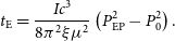 \begin{equation} t_\mathrm{E} = \frac{Ic^3}{8\pi^2\xi \mu^2}\left(P_\mathrm{EP}^2 - P_0^2\right).\end{equation}
If
 $P_\mathrm{EP} \gg P_0$
, then
$P_\mathrm{EP} \gg P_0$
, then
 $t_\mathrm{E} \approx Ic / (4\mu\sqrt{\xi\dot{{\mathrm{M}}}v}) \approx$
 $\approx 2\times 10^7 B_{14}^{-1}v_2 n^{-1/2}$
yrs.
$\approx 2\times 10^7 B_{14}^{-1}v_2 n^{-1/2}$
yrs.
To obtain the duration of the propeller stage we integrate Equation (1) using
 $K_\mathrm{P}$
in the form of Equation (13) for case A and Equation (14) for case B. Thus, the duration of the propeller stage can be expressed as follows:
$K_\mathrm{P}$
in the form of Equation (13) for case A and Equation (14) for case B. Thus, the duration of the propeller stage can be expressed as follows:
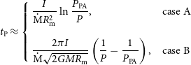 \begin{equation} t_\mathrm{P} \approx \left\{ \begin {array} {l@{\quad}l} \displaystyle \frac{I}{\dot{{\mathrm{M}}}R_\mathrm{m}^2} \ln{\frac{P_\mathrm{PA}}{P}}, & \mathrm{case\ A} \\[15pt] \displaystyle \frac{2\pi I}{\dot{{\mathrm{M}}}\sqrt{2GMR_\mathrm{m}}}\left(\frac{1}{P}-\frac{1}{P_\mathrm{PA}}\right), & \mathrm{case\ B} \\ \end {array} \right.\end{equation}
Here P represents the initial period at the propeller stage, so
 $P \ge P_\mathrm{EP}$
.
$P \ge P_\mathrm{EP}$
.
We numerically calculate several scenarios to obtain the dependence of the time required for the NS to become an accretor (
 $t_\mathrm{E} + t_\mathrm{P}$
) on the initial spin period
$t_\mathrm{E} + t_\mathrm{P}$
) on the initial spin period
 $P_0$
. These scenarios include NSs with different magnetic field values and are shown in Figure 1. To make our calculations more precise we choose only the lowest value of velocity,
$P_0$
. These scenarios include NSs with different magnetic field values and are shown in Figure 1. To make our calculations more precise we choose only the lowest value of velocity,
 $v=30$
km s
$v=30$
km s
 $^{-1}$
, assuming that low-velocity NSs have the highest chance to remain in the Galaxy disc, where the number density is
$^{-1}$
, assuming that low-velocity NSs have the highest chance to remain in the Galaxy disc, where the number density is
 $n\approx0.3$
cm
$n\approx0.3$
cm
 $^{-3}$
and remains approximately constant. For illustrative purposes, we calculate only case B of propeller spin down and show only field decay models CF and ED.
$^{-3}$
and remains approximately constant. For illustrative purposes, we calculate only case B of propeller spin down and show only field decay models CF and ED.
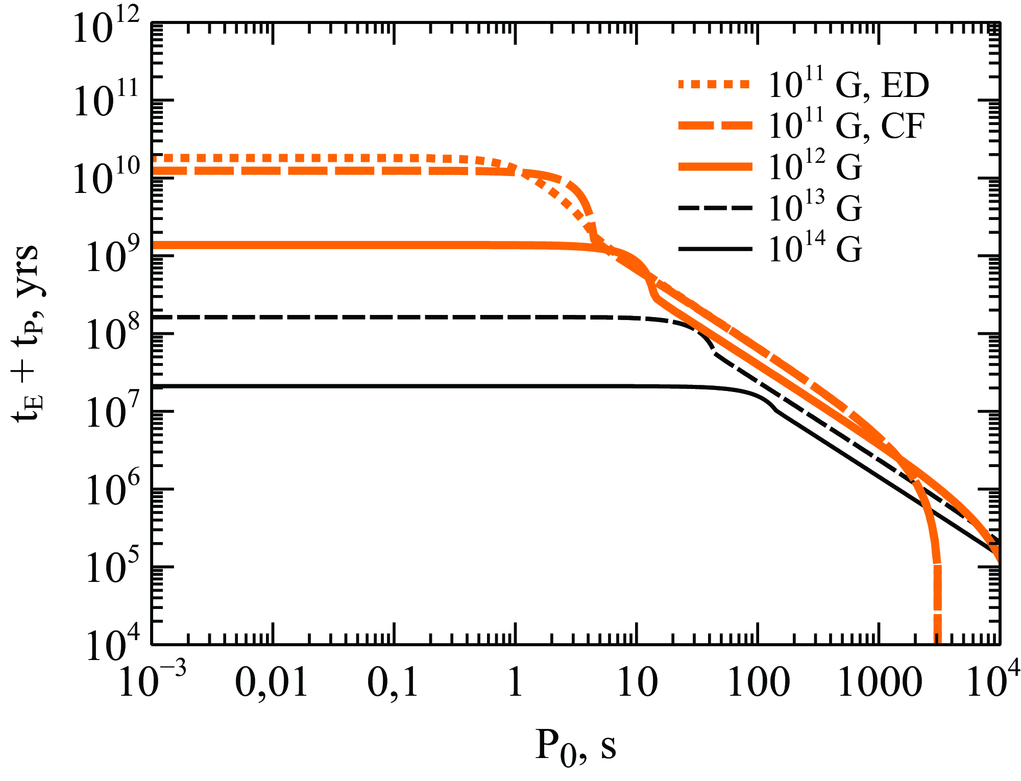
Figure 1. The time for the NS to reach the accretor stage, which is assumed to be the total duration of the ejector and propeller stages
 $t_E+t_P$
versus the initial spin period
$t_E+t_P$
versus the initial spin period
 $P_0$
. The results are shown for case B of propeller spin down,
$P_0$
. The results are shown for case B of propeller spin down,
 $v=30$
km/s,
$v=30$
km/s,
 $n=0.3$
cm
$n=0.3$
cm
 $^{-3}$
. We show two decay models only for
$^{-3}$
. We show two decay models only for
 $10^{11}$
G, since for the larger magnetic field values these two models lead to almost the same results of
$10^{11}$
G, since for the larger magnetic field values these two models lead to almost the same results of
 $t_E+t_P$
.
$t_E+t_P$
.
Now, we will examine the obtained results. In most cases
 $t_\mathrm{E} > t_\mathrm{P}$
, hence the total duration
$t_\mathrm{E} > t_\mathrm{P}$
, hence the total duration
 $t_\mathrm{E} + t_\mathrm{P}$
of NSs with low initial spin periods depends mostly on
$t_\mathrm{E} + t_\mathrm{P}$
of NSs with low initial spin periods depends mostly on
 $t_\mathrm{E}$
. The total duration remains almost the same until
$t_\mathrm{E}$
. The total duration remains almost the same until
 $P_0$
becomes comparable to
$P_0$
becomes comparable to
 $P_\mathrm{EP}$
, since
$P_\mathrm{EP}$
, since
 $t_\mathrm{E}$
has a weak dependence on
$t_\mathrm{E}$
has a weak dependence on
 $P_0$
if
$P_0$
if
 $P_0 \ll P_\mathrm{EP}$
(Equation 25). As
$P_0 \ll P_\mathrm{EP}$
(Equation 25). As
 $P_0$
approaches
$P_0$
approaches
 $P_\mathrm{EP}$
, the duration of the ejector stage decreases and at some point becomes comparable to the duration of the propeller stage. As soon as
$P_\mathrm{EP}$
, the duration of the ejector stage decreases and at some point becomes comparable to the duration of the propeller stage. As soon as
 $t_\mathrm{E}$
and
$t_\mathrm{E}$
and
 $t_\mathrm{P}$
are equal, we see a break in the curves. For greater values of
$t_\mathrm{P}$
are equal, we see a break in the curves. For greater values of
 $P_0$
the total duration is determined by
$P_0$
the total duration is determined by
 $t_\mathrm{P}$
and has a stronger dependence on the initial spin period. If
$t_\mathrm{P}$
and has a stronger dependence on the initial spin period. If
 $P_0 > P_\mathrm{EP}$
, the NS starts its evolution from the propeller stage and
$P_0 > P_\mathrm{EP}$
, the NS starts its evolution from the propeller stage and
 $t_\mathrm{E} = 0$
. After
$t_\mathrm{E} = 0$
. After
 $P_0 > P_\mathrm{PA}$
, the total duration is assumed to be zero, since the NS starts as an accretor. This situation is realised for
$P_0 > P_\mathrm{PA}$
, the total duration is assumed to be zero, since the NS starts as an accretor. This situation is realised for
 $B_0 = 10^{11}$
G,
$B_0 = 10^{11}$
G,
 $P_0 \gtrsim 3\,000$
s. Generally, the duration of both the ejector and propeller stages decreases with the increase in
$P_0 \gtrsim 3\,000$
s. Generally, the duration of both the ejector and propeller stages decreases with the increase in
 $B_0$
. As for magnetic field decay, it changes the result only if the total duration is noticeably greater than the characteristic decay timescale. This is realised for
$B_0$
. As for magnetic field decay, it changes the result only if the total duration is noticeably greater than the characteristic decay timescale. This is realised for
 $10^{11}$
G,
$10^{11}$
G,
 $P_0 \lesssim 10$
s, since
$P_0 \lesssim 10$
s, since
 $t_\mathrm{E} + t_\mathrm{P} > \tau_\mathrm{Ohm} \sim 10^9$
years. For
$t_\mathrm{E} + t_\mathrm{P} > \tau_\mathrm{Ohm} \sim 10^9$
years. For
 $B_0 > 10^{11}$
G the field decay effect is negligible for the models that we analyse.
$B_0 > 10^{11}$
G the field decay effect is negligible for the models that we analyse.
To follow the evolution of the NS rotation in more detail, we model 48 scenarios of the evolution of the INS spin-down: 2 variants of the propeller spin-down
 $\times$
2 values of the velocity v
$\times$
2 values of the velocity v
 $\times$
3 models of the magnetic field decay
$\times$
3 models of the magnetic field decay
 $\times$
4 values of the initial magnetic field. All of them are presented in Figures 2 and 3 for the propeller models A and B, correspondingly.
$\times$
4 values of the initial magnetic field. All of them are presented in Figures 2 and 3 for the propeller models A and B, correspondingly.
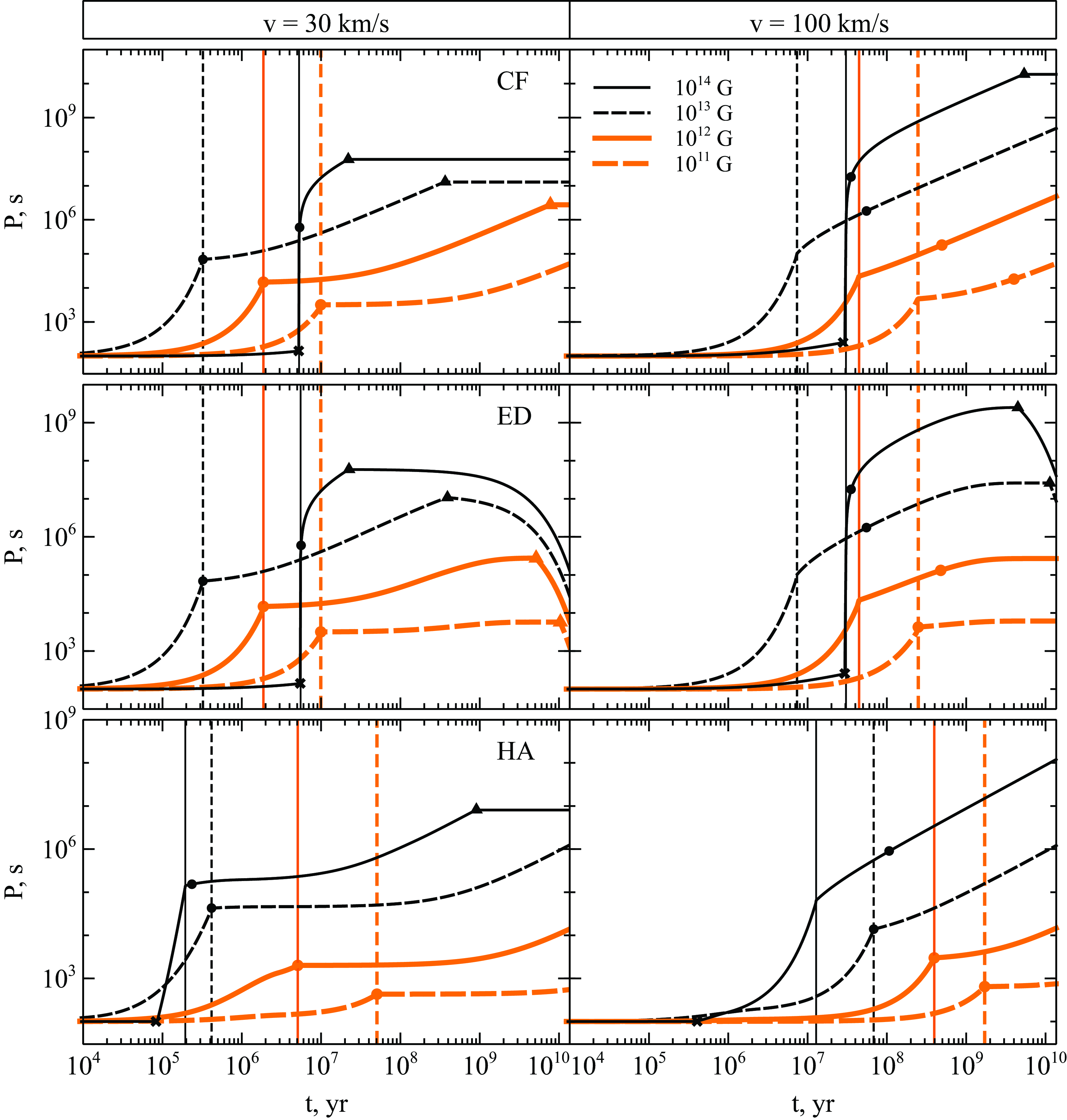
Figure 2. The spin period evolution for the case A of propeller spin-down (Equation 13). Two columns correspond to different values of the velocity v. Three rows represent different magnetic field evolution models: constant field (CF) – top, exponential decay (ED) – middle, and Hall attractor (HA) – bottom. Each line style corresponds to an initial magnetic field value
 $B_0$
. Vertical lines correspond to the onset of accretion at
$B_0$
. Vertical lines correspond to the onset of accretion at
 $t_{\mathrm{PA}}$
for every curve. An ejector-propeller transition of NS with
$t_{\mathrm{PA}}$
for every curve. An ejector-propeller transition of NS with
 $B_0 = 10^{14}$
G is seen as a cross. A filled circle on each curve is for the time
$B_0 = 10^{14}$
G is seen as a cross. A filled circle on each curve is for the time
 $t_{\mathrm{cr}}$
and the period
$t_{\mathrm{cr}}$
and the period
 $P_{\mathrm{cr}}$
. After the time
$P_{\mathrm{cr}}$
. After the time
 $t_{\mathrm{cr}}$
is reached the NS enters the turbulent regime and can also reach the turbulent period
$t_{\mathrm{cr}}$
is reached the NS enters the turbulent regime and can also reach the turbulent period
 $P_{\mathrm{turb}}$
at
$P_{\mathrm{turb}}$
at
 $t=t_{\mathrm{turb}}$
, which corresponds to a triangle.
$t=t_{\mathrm{turb}}$
, which corresponds to a triangle.
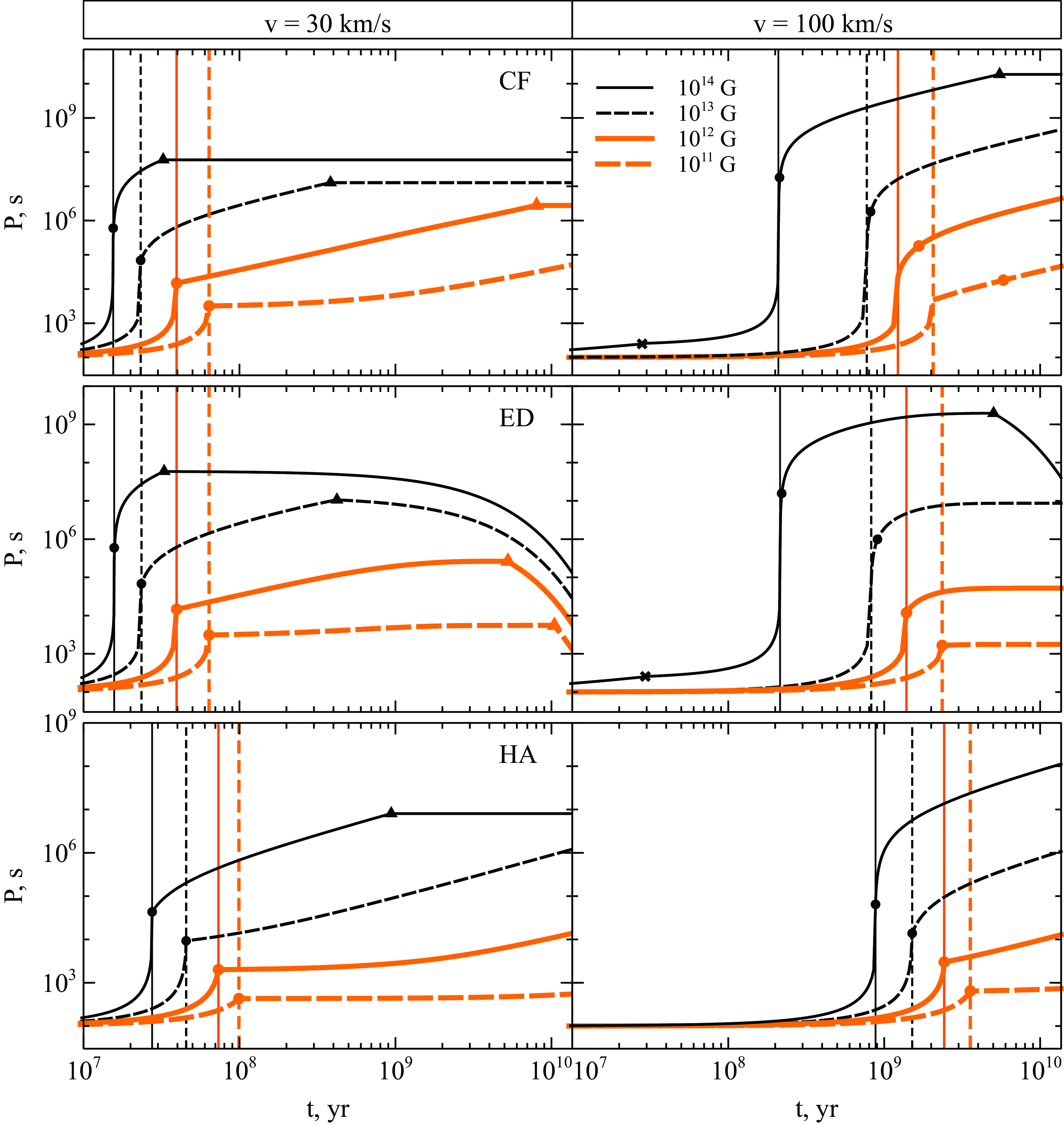
Figure 3. The spin period evolution for the case B of propeller spin-down (Equation 14). An ejector-propeller transition of NS with
 $B_0 = 10^{14}$
G is shown as a cross. Vertical lines show the onset of accretion for each NS (
$B_0 = 10^{14}$
G is shown as a cross. Vertical lines show the onset of accretion for each NS (
 $t_{\mathrm{PA}}$
). Filled circles correspond to the start of a turbulent regime (
$t_{\mathrm{PA}}$
). Filled circles correspond to the start of a turbulent regime (
 $P_{\mathrm{cr}}$
,
$P_{\mathrm{cr}}$
,
 $t_{\mathrm{cr}}$
). The reaching of
$t_{\mathrm{cr}}$
). The reaching of
 $P_{\mathrm{turb}}$
is shown as filled triangles. Line styles and colours are the same as in Figure 2.
$P_{\mathrm{turb}}$
is shown as filled triangles. Line styles and colours are the same as in Figure 2.
At each plot, we show P(t) curves for different initial magnetic fields
 $B_0$
assuming one of the models of the magnetic field decay – either constant field (CF) or exponential decay (ED) or Hall attractor (HA). For each curve, we mark moments of time
$B_0$
assuming one of the models of the magnetic field decay – either constant field (CF) or exponential decay (ED) or Hall attractor (HA). For each curve, we mark moments of time
 $t_\mathrm{PA}$
of the propeller-accretor transition by the vertical line of a corresponding style. Also, we use filled circles to mark moments of time
$t_\mathrm{PA}$
of the propeller-accretor transition by the vertical line of a corresponding style. Also, we use filled circles to mark moments of time
 $t_\mathrm{cr}$
when the turbulence of ISM becomes important. Triangles indicate the reaching of an equilibrium for each NS. The ejector-propeller transition is marked with crosses. For the constant magnetic field model, we summarise all these times (and corresponding periods) in Table 1.
$t_\mathrm{cr}$
when the turbulence of ISM becomes important. Triangles indicate the reaching of an equilibrium for each NS. The ejector-propeller transition is marked with crosses. For the constant magnetic field model, we summarise all these times (and corresponding periods) in Table 1.
Generally, we conclude, that an INS with parameters under study would become an accretor in
 ${\sim} 10^5-10^9$
years of evolution.
${\sim} 10^5-10^9$
years of evolution.
Below we describe the properties of each stage as we get it from our calculations.
Ejector. In our calculations each INS starts its evolution with an initial period of 100 s. The combination of the velocity v and the initial magnetic field
 $B_0$
defines the first stage, since both of the transition periods
$B_0$
defines the first stage, since both of the transition periods
 $P_{\mathrm{EP}}$
and
$P_{\mathrm{EP}}$
and
 $P_{\mathrm{PA}}$
depend on these parameters. As it is noticed by Afonina, Biryukov, & Popov (Reference Afonina, Biryukov and Popov2023), long-period INSs with
$P_{\mathrm{PA}}$
depend on these parameters. As it is noticed by Afonina, Biryukov, & Popov (Reference Afonina, Biryukov and Popov2023), long-period INSs with
 $B \lesssim 10^{13}$
G in a typical ISM cannot be at the ejector stage. For both adopted velocity values, only NSs with the magnetic field
$B \lesssim 10^{13}$
G in a typical ISM cannot be at the ejector stage. For both adopted velocity values, only NSs with the magnetic field
 $10^{14}$
G start their evolution at the ejector stage. In all other cases, NSs start as propellers. Therefore, on every plot, the early spin-down of NSs with
$10^{14}$
G start their evolution at the ejector stage. In all other cases, NSs start as propellers. Therefore, on every plot, the early spin-down of NSs with
 $B_0 = 10^{11}, 10^{12}$
, and
$B_0 = 10^{11}, 10^{12}$
, and
 $10^{13}$
G obeys the propeller spin-down law, and the NS with the magnetic field
$10^{13}$
G obeys the propeller spin-down law, and the NS with the magnetic field
 $10^{14}$
G undergoes ejector spin-down. On the other hand, all modelled NSs end their evolution as accretors.
$10^{14}$
G undergoes ejector spin-down. On the other hand, all modelled NSs end their evolution as accretors.
The transition to the propeller stage occurs when
 $P = P_{\mathrm{EP}}$
. The corresponding moment of time
$P = P_{\mathrm{EP}}$
. The corresponding moment of time
 $t_\mathrm{EP}$
depends on the specific combination of v,
$t_\mathrm{EP}$
depends on the specific combination of v,
 $B_0$
, and the adopted field decay model. For instance, for models CF and ED the transition time is almost exactly the same:
$B_0$
, and the adopted field decay model. For instance, for models CF and ED the transition time is almost exactly the same:
 $t_\mathrm{EP} = 5\times 10^6$
yrs. This is so because the characteristic decay timescale for the ED model is long –
$t_\mathrm{EP} = 5\times 10^6$
yrs. This is so because the characteristic decay timescale for the ED model is long –
 $\tau_{\mathrm{Ohm}} \approx 10^9 \gg 10^6$
yrs – and therefore, the NSs’ parameters in both cases (A and B) are similar during the ejector-propeller transition. On the contrary, for the HA model
$\tau_{\mathrm{Ohm}} \approx 10^9 \gg 10^6$
yrs – and therefore, the NSs’ parameters in both cases (A and B) are similar during the ejector-propeller transition. On the contrary, for the HA model
 $t_\mathrm{EP} \sim 10^6$
yrs which is comparable to the field decay timescale. So, the change to the propeller in the HA case occurs due to field decay, which leads to a decrease of
$t_\mathrm{EP} \sim 10^6$
yrs which is comparable to the field decay timescale. So, the change to the propeller in the HA case occurs due to field decay, which leads to a decrease of
 $R_{\mathrm{Sh}}$
. Therefore, the condition
$R_{\mathrm{Sh}}$
. Therefore, the condition
 $R_{\mathrm{Sh}}=R_{\mathrm{G}}$
is fulfilled earlier, since
$R_{\mathrm{Sh}}=R_{\mathrm{G}}$
is fulfilled earlier, since
 $R_{\mathrm{G}}$
is constant. So, for the NS with
$R_{\mathrm{G}}$
is constant. So, for the NS with
 $B_0=10^{14}$
G and the HA model (two bottom panels in both Figures) the transition to the propeller stage occurs due to the field decay rather than spin-down due to pulsar losses.
$B_0=10^{14}$
G and the HA model (two bottom panels in both Figures) the transition to the propeller stage occurs due to the field decay rather than spin-down due to pulsar losses.
Propeller. Let us consider first the propeller stage of an NS with an initial magnetic field strength of
 $B_0 = 10^{14}$
G. In case A, the energy loss rate of the propeller is significantly greater than that of the ejector. So, the spin-down rate changes dramatically, as indicated by the break in lines for
$B_0 = 10^{14}$
G. In case A, the energy loss rate of the propeller is significantly greater than that of the ejector. So, the spin-down rate changes dramatically, as indicated by the break in lines for
 $10^{14}$
G. In this case, within model A and for field decay models CF and ED, the duration of the propeller stage is much shorter than the duration of the ejector stage. As a result, the period increases very rapidly by approximately three orders of magnitude in a rather short time. Thus, for CF and ED and for
$10^{14}$
G. In this case, within model A and for field decay models CF and ED, the duration of the propeller stage is much shorter than the duration of the ejector stage. As a result, the period increases very rapidly by approximately three orders of magnitude in a rather short time. Thus, for CF and ED and for
 $v = 30$
km s
$v = 30$
km s
 $^{-1}$
the propeller stage starts at
$^{-1}$
the propeller stage starts at
 ${\sim} 5 \times 10^{6}$
yrs and lasts only for
${\sim} 5 \times 10^{6}$
yrs and lasts only for
 ${\lesssim} 10^{5}$
yrs, while the period P changes from 140 s to
${\lesssim} 10^{5}$
yrs, while the period P changes from 140 s to
 $3\times10^5$
s during this stage. On the other hand, for the HA field evolution model, the duration of this stage is comparable to that of the ejector due to magnetic field decay, which makes the deceleration less effective.
$3\times10^5$
s during this stage. On the other hand, for the HA field evolution model, the duration of this stage is comparable to that of the ejector due to magnetic field decay, which makes the deceleration less effective.
As for models with
 $B_0 < 10^{14}$
G, all of them start their evolution as propellers. For cases A and B, the weaker the magnetic field the slower the spin-down.
$B_0 < 10^{14}$
G, all of them start their evolution as propellers. For cases A and B, the weaker the magnetic field the slower the spin-down.
Let us note the difference between the HA model and other field decay models for cases A and B. For the HA model, the characteristic decay timescale
 ${\sim}10^{6}$
yrs is comparable to
${\sim}10^{6}$
yrs is comparable to
 $t_{\mathrm{PA}} \sim 2\times10^5-5\times10^6$
yrs in case A. Therefore, it affects the period evolution. On the contrary, in the case B
$t_{\mathrm{PA}} \sim 2\times10^5-5\times10^6$
yrs in case A. Therefore, it affects the period evolution. On the contrary, in the case B
 $t_{\mathrm{PA}} \gtrsim 2\times10^7$
yrs is much greater than the decay timescale for every
$t_{\mathrm{PA}} \gtrsim 2\times10^7$
yrs is much greater than the decay timescale for every
 $B_0$
and v values considered in this work. So, the transition to the propeller stage and further evolution is almost the same as it would be with a constant field of the value
$B_0$
and v values considered in this work. So, the transition to the propeller stage and further evolution is almost the same as it would be with a constant field of the value
 $B \approx 0.05 B_0$
.
$B \approx 0.05 B_0$
.
Now we consider the difference of the propeller-accretor transition of NSs with
 $B_0 = 10^{14}$
G and NSs with smaller initial magnetic fields. For model HA of case A and all decay models of case B the ejector and propeller spin-down rate can be considered comparable. So, for larger
$B_0 = 10^{14}$
G and NSs with smaller initial magnetic fields. For model HA of case A and all decay models of case B the ejector and propeller spin-down rate can be considered comparable. So, for larger
 $B_0$
the propeller-accretor transition happens earlier. On the contrary, in models CF and ED of case A the propeller spin-down is much more effective. A NS with
$B_0$
the propeller-accretor transition happens earlier. On the contrary, in models CF and ED of case A the propeller spin-down is much more effective. A NS with
 $B_0 = 10^{14}$
G spends part of its early evolution at the ejector stage, while NSs with lower
$B_0 = 10^{14}$
G spends part of its early evolution at the ejector stage, while NSs with lower
 $B_0$
are born already at the propeller stage. This delays the propeller-accretor transition for the NS with
$B_0$
are born already at the propeller stage. This delays the propeller-accretor transition for the NS with
 $B_0 = 10^{14}$
G in comparison to the transition of NSs with lower magnetic fields.
$B_0 = 10^{14}$
G in comparison to the transition of NSs with lower magnetic fields.
While the value of the velocity v does not affect the ejector spin-down, the ejector-propeller transition period
 $P_{\mathrm{EP}} \propto v^{1/2}$
, so
$P_{\mathrm{EP}} \propto v^{1/2}$
, so
 $B_0=10^{14}$
G and either
$B_0=10^{14}$
G and either
 $v=30$
km s
$v=30$
km s
 $^{-1}$
or 100 km s
$^{-1}$
or 100 km s
 $^{-1}$
correspond to
$^{-1}$
correspond to
 $P_\mathrm{EP}\,=\,140$
s and 260 s, respectively. The latter makes the ejector stage longer. Thus, for field decay models CF and ED the duration of the ejector stage increases from
$P_\mathrm{EP}\,=\,140$
s and 260 s, respectively. The latter makes the ejector stage longer. Thus, for field decay models CF and ED the duration of the ejector stage increases from
 $5 \times 10^6$
yrs to
$5 \times 10^6$
yrs to
 $3 \times 10^7$
yrs. At the same time, the propeller stage is due to interaction with the ISM and corresponding spin-down laws depend on
$3 \times 10^7$
yrs. At the same time, the propeller stage is due to interaction with the ISM and corresponding spin-down laws depend on
 $\dot{{\mathrm{M}}} \propto v^{-3}$
. So, the propeller spin-down rate is much less effective for high velocities. The moment of the propeller-accretor transition also depends on v, although this dependence is rather weak (
$\dot{{\mathrm{M}}} \propto v^{-3}$
. So, the propeller spin-down rate is much less effective for high velocities. The moment of the propeller-accretor transition also depends on v, although this dependence is rather weak (
 $P_{\mathrm{PA}} \propto v^{1/3}$
). As a result, the transition to the accretor stage for all high-velocity cases occurs later than that for low-velocity ones. At the same time, lower
$P_{\mathrm{PA}} \propto v^{1/3}$
). As a result, the transition to the accretor stage for all high-velocity cases occurs later than that for low-velocity ones. At the same time, lower
 $P_\mathrm{PA}$
correspond to lower values of the magnetic field, as it follows from Equation (17) if v remains unchanged. Therefore, in our results, we see the accretor stage for high
$P_\mathrm{PA}$
correspond to lower values of the magnetic field, as it follows from Equation (17) if v remains unchanged. Therefore, in our results, we see the accretor stage for high
 $B_0$
starts at a longer period
$B_0$
starts at a longer period
 $P_{\mathrm{PA}}$
.
$P_{\mathrm{PA}}$
.
Bondi accretor. Now, let us consider the spin period evolution for
 $t > t_{\mathrm{PA}}$
. If the spin period becomes long enough, we have to account for the interstellar turbulence. The turbulent regime is reached when an NS spins down to the critical period
$t > t_{\mathrm{PA}}$
. If the spin period becomes long enough, we have to account for the interstellar turbulence. The turbulent regime is reached when an NS spins down to the critical period
 $P_{\mathrm{cr}}$
. At this moment the turbulent torque becomes comparable to the accretor spin-down torque given by Equation (18). Still, at the onset of the turbulent regime of the spin evolution, the NS is far from the equilibrium (the latter is expected since turbulence effectively spins up the star – see below). In Figures 2 and 3 the moments
$P_{\mathrm{cr}}$
. At this moment the turbulent torque becomes comparable to the accretor spin-down torque given by Equation (18). Still, at the onset of the turbulent regime of the spin evolution, the NS is far from the equilibrium (the latter is expected since turbulence effectively spins up the star – see below). In Figures 2 and 3 the moments
 $t = t_{\mathrm{cr}}$
when
$t = t_{\mathrm{cr}}$
when
 $P = P_{\mathrm{cr}}$
are marked with filled circles on the curves.
$P = P_{\mathrm{cr}}$
are marked with filled circles on the curves.
In the situation, when the period
 $P_{\mathrm{cr}} < P_{\mathrm{PA}}$
we consider the turbulence to become significant right after the accretion starts and assume
$P_{\mathrm{cr}} < P_{\mathrm{PA}}$
we consider the turbulence to become significant right after the accretion starts and assume
 $P_{\mathrm{cr}} = P_{\mathrm{PA}}$
and
$P_{\mathrm{cr}} = P_{\mathrm{PA}}$
and
 $t_{\mathrm{cr}} = t_{\mathrm{PA}}$
. The condition
$t_{\mathrm{cr}} = t_{\mathrm{PA}}$
. The condition
 $P_{\mathrm{cr}} < P_{\mathrm{PA}}$
is satisfied for NSs with
$P_{\mathrm{cr}} < P_{\mathrm{PA}}$
is satisfied for NSs with
 $v = 30\,\mathrm{km\,s}^{-1}$
. On the other hand, the turbulent regime starts later for
$v = 30\,\mathrm{km\,s}^{-1}$
. On the other hand, the turbulent regime starts later for
 $v = 100\,\mathrm{km\,s}^{-1}$
, as can be seen from Table 1. This is so as
$v = 100\,\mathrm{km\,s}^{-1}$
, as can be seen from Table 1. This is so as
 $P_{\mathrm{cr}} \propto v^{17/6}$
, thus it depends much stronger on v than
$P_{\mathrm{cr}} \propto v^{17/6}$
, thus it depends much stronger on v than
 $P_{\mathrm{PA}} \propto v^{1/3}$
.
$P_{\mathrm{PA}} \propto v^{1/3}$
.
Turbulent regime. The spin period evolution after reaching the turbulent regime at
 $t_{\mathrm{cr}}$
is influenced by the turbulence. How quickly the turbulent regime is established depends on the spin-down torque. In the case of settling accretion, it happens much faster, on a time scale comparable to the duration of the propeller regime under the torque defined by Equation (13). In the case of Bondi accretion, the turbulent regime appears later. Below we present the results for this assumption.
$t_{\mathrm{cr}}$
is influenced by the turbulence. How quickly the turbulent regime is established depends on the spin-down torque. In the case of settling accretion, it happens much faster, on a time scale comparable to the duration of the propeller regime under the torque defined by Equation (13). In the case of Bondi accretion, the turbulent regime appears later. Below we present the results for this assumption.
Due to the existence of stochastic turbulent torque, the NS spin evolution can not be described only with the accretor spin-down torque, Equation (18). So, the stellar spin period obtained in our calculations after
 $t_\mathrm{turb}$
can be interpreted as an upper bound value. Therefore, we actually give only a lower bound for the time (
$t_\mathrm{turb}$
can be interpreted as an upper bound value. Therefore, we actually give only a lower bound for the time (
 $t_{\mathrm{turb}}$
) of reaching the equilibrium. In Figures 2 and 3 the moments
$t_{\mathrm{turb}}$
) of reaching the equilibrium. In Figures 2 and 3 the moments
 $t = t_{\mathrm{turb}}$
when
$t = t_{\mathrm{turb}}$
when
 $P = P_{\mathrm{turb}}$
are marked with triangles on the curves.
$P = P_{\mathrm{turb}}$
are marked with triangles on the curves.
In general, the stronger the magnetic field B and the lower the velocity v, the earlier an NS reaches
 $P_{\mathrm{turb}}$
. For instance, in cases A and B for models CF and ED the NS with
$P_{\mathrm{turb}}$
. For instance, in cases A and B for models CF and ED the NS with
 $B_0=10^{14}$
G reaches the equilibrium, while for lower initial magnetic field values it is not necessarily true. For example, for CF, as shown in Table 1, the NS with the lowest magnetic field
$B_0=10^{14}$
G reaches the equilibrium, while for lower initial magnetic field values it is not necessarily true. For example, for CF, as shown in Table 1, the NS with the lowest magnetic field
 $10^{11}$
G does not reach the equilibrium period for both velocity values.
$10^{11}$
G does not reach the equilibrium period for both velocity values.
In contrast with CF and ED models, an NS within the HA model reaches the equilibrium later, despite the fact that
 $P_{\mathrm{turb}}$
in these cases does not vary significantly. That is so because the spin-down rate at the accretor stage depends on the magnetic field value. After
$P_{\mathrm{turb}}$
in these cases does not vary significantly. That is so because the spin-down rate at the accretor stage depends on the magnetic field value. After
 ${\sim}$
few
${\sim}$
few
 $\times 10^{5}$
–
$\times 10^{5}$
–
 ${\sim}$
few
${\sim}$
few
 $\times 10^{6}$
yrs the magnetic field in the HA model decreases down to
$\times 10^{6}$
yrs the magnetic field in the HA model decreases down to
 $\approx 0.05 B_0$
. Thus, the drop in the B value results in slowing down the increase of the period. As for velocity values,
$\approx 0.05 B_0$
. Thus, the drop in the B value results in slowing down the increase of the period. As for velocity values,
 $P_{\mathrm{turb}}$
is highly dependent on v (
$P_{\mathrm{turb}}$
is highly dependent on v (
 $P_{\mathrm{turb}} \propto v^{43/9}$
). So, NSs with
$P_{\mathrm{turb}} \propto v^{43/9}$
). So, NSs with
 $v = 100\,\mathrm{km\,s}^{-1}$
reach the equilibrium regime later than NSs with
$v = 100\,\mathrm{km\,s}^{-1}$
reach the equilibrium regime later than NSs with
 $v = 30\,\mathrm{km\,s}^{-1}$
. After the equilibrium period is reached, we assume
$v = 30\,\mathrm{km\,s}^{-1}$
. After the equilibrium period is reached, we assume
 $P = P_{\mathrm{turb}}$
. For the CF model,
$P = P_{\mathrm{turb}}$
. For the CF model,
 $P_{\mathrm{turb}}$
does not change with time, because for this model B is constant. In the HA model, after
$P_{\mathrm{turb}}$
does not change with time, because for this model B is constant. In the HA model, after
 $P_{\mathrm{turb}}$
is reached, the magnetic field value is also constant because the field decays to its final value of
$P_{\mathrm{turb}}$
is reached, the magnetic field value is also constant because the field decays to its final value of
 $\approx 0.05 B_0$
in
$\approx 0.05 B_0$
in
 $10^{6}$
yrs which is
$10^{6}$
yrs which is
 $\ll t_{\mathrm{turb}}$
. After
$\ll t_{\mathrm{turb}}$
. After
 $t_{\mathrm{turb}}$
the field decay continues only for the ED model. Here the noticeable decrease in B occurs at a time
$t_{\mathrm{turb}}$
the field decay continues only for the ED model. Here the noticeable decrease in B occurs at a time
 ${\sim} 10^9$
yrs. This can be seen as a decrease in
${\sim} 10^9$
yrs. This can be seen as a decrease in
 $P_{\mathrm{turb}}$
in the middle panels of both Figures.
$P_{\mathrm{turb}}$
in the middle panels of both Figures.

5. Discussion
In this paper, we aimed to study the long-term evolution of INSs with long initial spin periods
 ${\sim} 100$
s focusing on their transition to the stage of accretion. Inevitably, we made many simplifying assumptions. Some of them are discussed here.
${\sim} 100$
s focusing on their transition to the stage of accretion. Inevitably, we made many simplifying assumptions. Some of them are discussed here.
The main simplification is related to the usage of constant spatial velocities and ISM density. Previous calculations (e.g., Popov et al., Reference Popov, Colpi, Treves, Turolla, Lipunov and Prokhorov2000) demonstrated that detailed calculations of the spatial evolution are important. Still, basic properties of the evolution of INSs with potentially larger luminosity at the accretion stage can be calculated under these assumptions, as these objects have low spatial velocities of about a few tens of km per second. So, they spend their lives close to the Galactic plane. However, the short duration of pre-accretor stages for NSs with long initial spin periods demonstrate that such objects can reach the accretor phase of evolution even if they spend just a part of their lives in a high-density environment in the Galactic disc. Our preliminary calculations indicate that NSs with standard initial periods (
 $P_0\lesssim1$
s) and magnetic fields (
$P_0\lesssim1$
s) and magnetic fields (
 $B\sim 10^{11} - 10^{12}$
G) would not start to accrete if they spend a significant part of their lives above the Galactic plane. In the future, we plan to include details of spatial evolution in order to make a realistic population model.
$B\sim 10^{11} - 10^{12}$
G) would not start to accrete if they spend a significant part of their lives above the Galactic plane. In the future, we plan to include details of spatial evolution in order to make a realistic population model.
In this study, we used three very simple models of the magnetic field evolution. Contrary to the assumptions discussed before, here we are limited by uncertainties in the long-term field behaviour. Potentially, it is possible to implement a more detailed treatment of the evolution of the magnetic field accounting for the thermal evolution which influences the Ohmic time scale, for the evolution of the field in the core, etc. Still, uncertainties are so big that we think that it is premature to apply sophisticated scenarios.
Now let us discuss some issues related to our treatment of spin evolution. At first, we used the traditional treatment of the centrifugal barrier with the critical condition
 $R_{\mathrm{c}}=R_{\mathrm{m}}$
where
$R_{\mathrm{c}}=R_{\mathrm{m}}$
where
 $R_{\mathrm{c}}$
is calculated according to Equation (11). This standard approach was recently challenged by Lyutikov (Reference Lyutikov2023). The author demonstrated that for dipolar magnetically aligned case the critical radius is
$R_{\mathrm{c}}$
is calculated according to Equation (11). This standard approach was recently challenged by Lyutikov (Reference Lyutikov2023). The author demonstrated that for dipolar magnetically aligned case the critical radius is
 $(2/3)^{1/3}R_{\mathrm{c}}$
. Accounting for this effect might make the propeller stage longer. However, we notice that there are many significant uncertainties in the spin-down rate at this stage. Our estimates demonstrate that in our study uncertainties in the spin-down rate are more important than the critical condition for the transition from propeller to accretor.
$(2/3)^{1/3}R_{\mathrm{c}}$
. Accounting for this effect might make the propeller stage longer. However, we notice that there are many significant uncertainties in the spin-down rate at this stage. Our estimates demonstrate that in our study uncertainties in the spin-down rate are more important than the critical condition for the transition from propeller to accretor.
In our opinion, the most crucial uncertainties in calculating the time of the onset of accretion are related to the rate of spin-down at the propeller stage. We also make calculations for cases C and D. For them we obtain that the time needed for an NS to start accretion is longer than the Galactic age:
 $t_{\mathrm{PA}} > t_{\mathrm{gal}}$
.
$t_{\mathrm{PA}} > t_{\mathrm{gal}}$
.
Davies & Pringle (Reference Davies and Pringle1981) suggested that accretion does not start immediately after the condition
 $R_{\mathrm{c}}=R_{\mathrm{m}}$
is reached. After a standard (supersonic) propeller there might be another stage – subsonic propeller. In our study, we ignore this stage. In our opinion, the heating balance in the envelope around the magnetosphere is adequately calculated in the settling accretion model. Thus, when
$R_{\mathrm{c}}=R_{\mathrm{m}}$
is reached. After a standard (supersonic) propeller there might be another stage – subsonic propeller. In our study, we ignore this stage. In our opinion, the heating balance in the envelope around the magnetosphere is adequately calculated in the settling accretion model. Thus, when
 $R_{\mathrm{m}}<R_{\mathrm{c}}$
in the low luminosity case realised in the case of AINSs the settling accretion model can applied. Additionally, up to our knowledge, the existence of the subsonic propeller stage is not supported by numerical calculations.
$R_{\mathrm{m}}<R_{\mathrm{c}}$
in the low luminosity case realised in the case of AINSs the settling accretion model can applied. Additionally, up to our knowledge, the existence of the subsonic propeller stage is not supported by numerical calculations.
Regarding the turbulent regime of accretion, we have to note that the details of the interaction of the heated envelope with turbulent matter captured within the settling accretion are poorly known. They are far beyond the scope of our study. Thus, we leave it to future analysis.
Now, we want to discuss some properties of AINSs. Postnov, & Shakura (Reference Popov, Postnov and Shakura2015) proposed that AINSs can be observed as transient sources. In our model, we do not account for the transient behaviour of these sources. Potentially, transient accretion can influence the spin behaviour of AINSs.
As we mentioned several times, already, there are numerous uncertainties in the properties and evolution of old INSs. Only observations of these sources can shed light on many issues. Unfortunately, the eROSITA survey is not completed and all observations with this instrument are stopped. In the near future, important results can be obtained thanks to numerous discoveries of INSs via microlensing with the Roman Telescope and other instruments, including Gaia (see e.g., (Lam et al., Reference Lam, Lu, Hosek, Dawson and Golovich2020) and references therein). Already many candidates for isolated compact objects are known (see e.g., (Mroz et al., Reference Mroz, Udalski, Wyrzykowski, Skowron, Poleski, Szymanski, Soszynski and Ulaczyk2021) and references therein). Deep X-ray and infrared observations of these sources by new space observatories can provide important upper limits or even detections.
Non-detection of AINSs even with the next generation of instruments can be explained by two reasons. Either INSs very seldom reach the stage of accretion, or the luminosity at this stage is lower than expected. Regime of low accretion with
 $\dot M \lesssim 10^{13}$
g s
$\dot M \lesssim 10^{13}$
g s
 $^{-1}$
potentially can be studied in binaries. In particular, in systems similar to those identified recently as binaries with invisible components with
$^{-1}$
potentially can be studied in binaries. In particular, in systems similar to those identified recently as binaries with invisible components with
 $M\sim 1.3-2.3 \, {\mathrm{M}_\odot}$
(Mazeh et al., Reference Mazeh, Faigler, Bashi, Shahaf, Davidson, Green and Gomel2022; Andrews, Taggart, & Foley, Reference Andrews, Taggart and Foley2022). If this question is clarified and if luminosities are not sufficiently low to explain the non-detection then the problem might be in the magneto-rotational evolution of INSs. If sources are not found then there can be several ways to explain it. For example, in the case of AINSs it can be due to properties of the propeller stage or/and due to magnetic field evolution. However, our results suggest that INSs with long initial spin periods can become accretors for various extreme variants of field behaviour. Thus, we suggest that the most probable evolutionary explanation for non-detection might be related to a prolonged propeller stage. Still, let us hope that AINSs will be identified shortly. This will give us lots of important information about the properties of NSs.
$M\sim 1.3-2.3 \, {\mathrm{M}_\odot}$
(Mazeh et al., Reference Mazeh, Faigler, Bashi, Shahaf, Davidson, Green and Gomel2022; Andrews, Taggart, & Foley, Reference Andrews, Taggart and Foley2022). If this question is clarified and if luminosities are not sufficiently low to explain the non-detection then the problem might be in the magneto-rotational evolution of INSs. If sources are not found then there can be several ways to explain it. For example, in the case of AINSs it can be due to properties of the propeller stage or/and due to magnetic field evolution. However, our results suggest that INSs with long initial spin periods can become accretors for various extreme variants of field behaviour. Thus, we suggest that the most probable evolutionary explanation for non-detection might be related to a prolonged propeller stage. Still, let us hope that AINSs will be identified shortly. This will give us lots of important information about the properties of NSs.
6. Conclusion
In this paper, we study the long-term behaviour of isolated NSs with long (
 ${\sim} 100$
s) initial spin periods for a range of initial magnetic fields, for different models of the field evolution, two values of the spatial velocity relative to the ISM, and constant external conditions. Our main goal is to calculate if INSs with such parameters can reach the stage of accretion of the interstellar gas within the Galactic age.
${\sim} 100$
s) initial spin periods for a range of initial magnetic fields, for different models of the field evolution, two values of the spatial velocity relative to the ISM, and constant external conditions. Our main goal is to calculate if INSs with such parameters can reach the stage of accretion of the interstellar gas within the Galactic age.
We find that the result strongly depends on the description of spin-down during the propeller stage. For realistic models with a rapid spin evolution at this stage (Davidson & Ostriker, Reference Davidson and Ostriker1973; Shakura, Reference Shakura1975), all INSs with reasonably low velocities (which potentially make it possible to have a relatively bright accretor) reach the stage of accretion in less than a few billion years.
Thus, we predict that if objects similar to PSR J0901-4046 (and, probably, GLEAM-X J1627-52 and GPM J1839-10) form a significant population of INSs in the Galaxy, then the expected number of isolated accretors is sufficiently increased in comparison to the predictions made in earlier studies.
Acknowledgement
We thank Prof. N.I. Shakura for discussions and the anonymous referee for useful comments and suggestions.
Funding statement
The work of M.A. and A.B. was supported by the RSF grant 21-12-00141. S.P. acknowledges support from the Simons Foundation.
Competing interests
None.
Data availability statement
The code used for modelling is accessible on request. Please, contact the first author.


