INTRODUCTION
Several types of adenovirus have been demonstrated to infect humans [Reference Ludwig1–Reference Gray3] and cause a wide variety of common and sporadic infections. Adenoviruses can infect various sites of the respiratory tract [Reference Brandt4], the gastrointestinal tract [Reference Bon5–Reference Oh, Gaedicke and Schreier7], and the eye [Reference Wishart8]. They can also infect the urinary bladder and the liver, although less frequently. Currently, there are 57 identified human adenovirus serotypes, which can be divided into seven subgenera (A–G) [Reference Wold, Ison, Knipe and Howley9]. It is not known why certain serotypes cause disease in some organs and not in others. The mechanisms of such tissue tropism or organ-specific pathogenicity cannot be explained by tissue culture experiments, animal models or bioinformatics analysis.
There is quite some information on the abundant presence of adenoviruses in the environment. It is well recognized that adenoviruses are very stable in watery suspension due to their well-organized capsid structure without envelope. They have been shown to remain infectious in several water types, such as surface, recreational and drinking water for a prolonged period of time, and have been shown to cause numerous waterborne outbreaks. It is therefore interesting to consider the health risks associated with their presence in the environment [Reference van Heerden10, Reference Choi and Jiang11].
If any adenovirus is found in an environmental water sample, and its concentration can be quantified [Reference Bofill-Mas12, Reference Wyn-Jones13], one may wish to translate human exposure into health risk. A complicating factor is found in the fact that adenovirus can infect humans via various exposure pathways. To predict the risk of infection, or the risk of acute symptoms given a certain (mode of) exposure, a dose-response relationship is needed. Aside from the magnitude of the dose, the probabilities of infection and illness may depend on the exposed mucosal tissues (the mode of exposure) and on the virus type, as well as on host factors determining susceptibility for that particular exposure mode.
Data on clinical consequences of human exposure to adenoviruses are uncommon, and for many pathogens there is limited information, usually from experiments with volunteers, done during the second half of the 20th century [Reference Teunis14, Reference Teunis, Brienen and Kretzschmar15]. From the literature, only five different adenovirus challenge studies are available. These studies used one virus type belonging to subgenus E (AdV4) and two different adenoviruses belonging to subgenus B (AdV7 and 16) that were inoculated via four different exposure modes: oral ingestion (Oral), inhalation (Inhal), intranasal (Nasal) and intraocular droplet inoculation (Ocul). For any of these virus type/exposure type combinations, a dose-response relationship could be described. Due to the diversity in conditions, any such dose-response model by virus/exposure type would be based on limited data and thus be highly uncertain.
The objective of this study was to develop a generalized dose-response model from these studies, to provide a basis for translating exposure to adenovirus into risk of infection and/or acute illness. By treating the set of dose-response studies as a (small) sample from the universe of adenovirus dose-response relationships. we may generalize the dose-response relationship from this collection of observed data. Using a hierarchical Bayesian framework, we will show that such generalization is possible and that, despite the small numbers of studies, we find meaningful differences in the effects of different exposure routes.
Adenovirus challenge studies data
The combined studies included a total of 91 subjects challenged in 23 dose groups. The studies are listed in Table 1 with information on dose, numbers exposed, numbers infected and numbers of subjects with acute illness symptoms.
Table 1. Adenovirus challenge studies with references. Three different virus types inoculated by four different pathways. Data include: estimated (mean) dose, numbers challenged (Exp), numbers shedding virus (Inf) and numbers of subjects with acute symptoms (Ill)
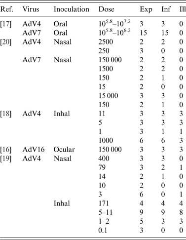
Titration of the inocula was similar in all papers: studies [Reference Kasel, Loda and Knight16–Reference Couch19] expressed dose in TCID50 units in human embryonic kidney cells, while study [Reference Hitchcock, Tyrrell and Bynoe20] reported TCID50 in pig kidney cells (PK).
Oral ingestion failed to produce any clinical symptoms [Reference Couch17], neither fever nor diarrhoea (one subject was reported to have had a brief diarrheal episode which was attributed to a different cause). Aerosol inoculation (Inhal) produced respiratory symptoms in the upper or lower respiratory tract (similar to pneumonia), sometimes accompanied by fever [Reference Couch18, Reference Couch19]. Intranasal inoculation did not produce any severe symptoms, some subjects had common cold-like symptoms that were attributed to other causes [Reference Hitchcock, Tyrrell and Bynoe20]. All subjects inoculated intra-ocularly developed conjuctivitis [Reference Kasel, Loda and Knight16].
It is worthwhile noting the considerable range in doses, and the differences in dosing schedules in the different experiments. It should also be noted that the data of oral and intra-ocular inoculation provide very limited information of the dose-response relationship.
METHODS
Dose-response models for infectious pathogens
Risk assessment rests on the analysis of conditional events: illness is conditional on (i.e. can only happen in) an infected host. Similarly, infection is conditional on exposure. Many human enteric pathogens infect their hosts at low doses: exposure to few organisms is associated with a considerable risk of infection [Reference Teunis21, Reference Thebault22]. As a consequence, the probability of exposure to at least a single infectious particle limits the probability of any health effect (infection, acute illness) in microbial dose-response assessment. At an average dose estimated from the concentration of suspended pathogens (c) multiplied by the inoculated volume (V), the probability of not ingesting even a single pathogen can be calculated. For instance, for a well-mixed (Poisson) suspension
At low doses this probability of exposure imposes a ‘natural’ limit to the risk of infection, independent of the infectivity of the pathogen or the susceptibility of the host [Reference Teunis and Havelaar23].
If any ingested pathogen has a fixed probability p m of surviving the chain of barriers to infection (numbered p 1, …, p m) the dose-response relationship for infection is
where the parameter p m quantifies host–pathogen interaction. When there is heterogeneity in this interaction (there usually is), a mixing distribution can be used, leading to the beta Poisson model for microbial infection
The dose-response relationship for the probability of acute symptoms in infected individuals (the conditional probability of illness, given infection) is defined as
based on the hazard of becoming ill, proportional to the duration of infection [Reference Teunis, Nagelkerke and Haas24].
Development of a generalized dose-response model
Within a single dose-response experiment the number of infected subjects is a binomial sample out of those exposed, with dose-dependent probability of infection
![]() $P_{{\rm inf}}(cV\vert\alpha, \beta )$
. Likewise, the number of symptomatic subjects is a binomial sample out of those infected, with dose-dependent probability
$P_{{\rm inf}}(cV\vert\alpha, \beta )$
. Likewise, the number of symptomatic subjects is a binomial sample out of those infected, with dose-dependent probability
![]() $P_{{\rm inf}\vert{\rm ill}}(cV\vert r,\eta )$
. The likelihood thus is the product of the two binomial probabilities, over all dose groups in the experiment.
$P_{{\rm inf}\vert{\rm ill}}(cV\vert r,\eta )$
. The likelihood thus is the product of the two binomial probabilities, over all dose groups in the experiment.
To let each separate dose-response experiment (by inoculation method and virus type) contribute to the generalized dose-response relationship, the data are analysed jointly in a hierarchical framework [Reference Teunis, Brienen and Kretzschmar15, Reference Teunis, Ogden and Strachan25]. Each study is thus assigned their own dose-response relationship, for infection as well as for illness. Variation in the infection parameters
![]() $(\alpha, \beta )$
and illness parameters
$(\alpha, \beta )$
and illness parameters
![]() $(r,\eta )$
in experiments is modelled by assuming they have a joint distribution. This joint distribution may be interpreted as the ‘group’-level distribution of infectivity and pathogenicity, with the data as a sample from the ‘universe’ of adenovirus dose-response relationships [Reference Teunis, Ogden and Strachan25].
$(r,\eta )$
in experiments is modelled by assuming they have a joint distribution. This joint distribution may be interpreted as the ‘group’-level distribution of infectivity and pathogenicity, with the data as a sample from the ‘universe’ of adenovirus dose-response relationships [Reference Teunis, Ogden and Strachan25].
To improve estimation, parameters were transformed as in [Reference Teunis, Takumi and Shinagawa26]:
so that we are estimating the mean value (u
1) of the beta distribution for p
m
and a quantity that is inversely related to its variance (for large positive v
1 the variance tends to zero). Further u
1 was logit-transformed and v
1 log-transformed. The illness parameters
![]() $(\eta, r)$
were given the same transformation.
$(\eta, r)$
were given the same transformation.
The effect of inoculation route was incorporated by assuming that the mean of the transformed parameter w 1, w 2 is categorical, where μ w 1,inoc and μ w 2,inoc can each have four different values, corresponding to the inoculation method (oral ingestion, intranasal droplet inoculation, aerosol inhalation, or intraocular droplet inoculation). As a simplifying assumption, the variation parameters z 1, z 2 were assumed to be the same for all eight experiments (as the small numbers of doses tested were not expected to allow assessment of the variation in infectivity and pathogenicity for each separate experiment).
The hierarchical model was implemented in a Bayesian framework, using normal priors for w
1, w
2 and z
1, z
2 with fixed s.d. = 2. Uncorrelated normal (mean = 0, s.d. = 4) hyperpriors were taken for
![]() $\mu _{w_1}$
,
$\mu _{w_1}$
,
![]() $\mu _{w_2}$
. Posterior parameter samples were obtained using JAGS [Reference Plummer27], controlled through rjags [Reference Plummer28] in R [29]. More details can be found in the last section of the Appendix.
$\mu _{w_2}$
. Posterior parameter samples were obtained using JAGS [Reference Plummer27], controlled through rjags [Reference Plummer28] in R [29]. More details can be found in the last section of the Appendix.
RESULTS
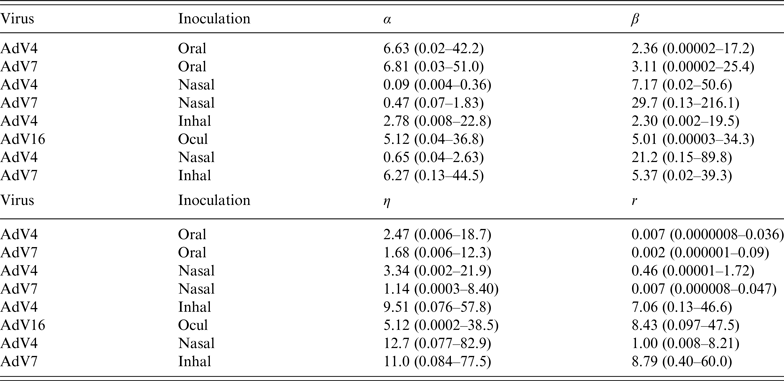
Parameter estimates are listed in Table 2, for the infectivity and conditional illness parameters by exposure category: oral ingestion, nasal droplet inoculation, aerosol inhalation, and ocular droplet inoculation. Estimates for the separate studies can be found in Appendix Table A1.
Table 2. Parameter estimates (mean and 95% range) for the adenovirus dose-response, by inoculation route: infectivity (infection dose-response) parameters (α, β) and pathogenicity (conditional illness dose-response) parameters (η, r)

Corresponding dose-response relationships are shown in Figures 1 and 2. Figure 1 shows the dose-response relationship for infection by exposure route. Although the 95% (posterior predictive) ranges appear similar, for intranasal droplet inoculation the estimated median probability of infection is lower as for the other three exposure pathways.
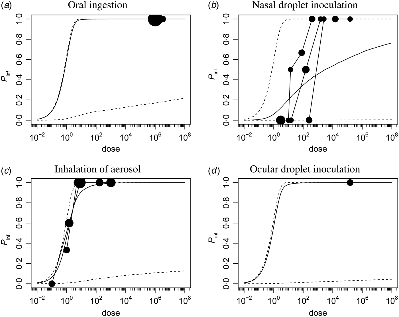
Fig. 1. Dose-response relationship for infection via the four different inoculation routes. Each graph shows the median and 95% range of the probability of infection as a function of dose, and any available data, as a bubble chart (symbol size proportional to the numbers challenged). Observations from the same study are connected.

Fig. 2. Dose-response relationship for illness via the four different inoculation routes. Each graph shows the median and 95% range of the (unconditional) probability of illness as a function of dose, and any available data, as a bubble chart (symbol size proportional to the numbers challenged). Observations from the same study are connected.
The probability of illness as a function of dose can be calculated by multiplying the infection probability [eqn (3)] and the conditional probability of illness given infection [eqn (4)]. Figure 2(a–d) shows these unconditional illness dose-response relationships for the four inoculation routes.
Here too the 95% (posterior predictive) intervals are similar, but the median curves indicate that oral and intranasal droplet exposure are less pathogenic than inhalation or ocular droplet exposure.
This pattern is confirmed by calculating the doses required to cause a 1% and a 50% risk, of infection and of illness. These predicted InfD01 and InfD50, and IllD01 and IllD50 are given in Figure 3. Corresponding numbers are tabulated in Table 3. The doses required for infection are low: few infectious virus particles; intranasal droplets appear less infectious. For acute symptoms, higher doses are necessary, with oral and intranasal droplets showing the lowest pathogenicity (i.e. the highest IllD01 and IllD50).

Fig. 3. Box plots of estimated doses for 1% and 50% probability of infection (a, b) and illness (c, d) via the four different exposure routes. Shown are median (horizontal line), quartiles (box) and 95% range (whiskers).
Table 3. Estimated dose required to cause 1% and 50% infection risk (InfD01 and InfD50) and 1% and 50% illness risk (IllD01 and IllD50) for adenovirus, by inoculation route: mean and 90% range

DISCUSSION
Data from five studies on three different adenovirus types and four different modes of inoculation were analysed jointly with separate dose-response models for infection and for illness (conditional on infection). The model was organized into four categories, representing the four different modes of inoculation: oral ingestion, intranasal droplet inoculation, inhalation of aerosolized virus, and intraocular droplet inoculation. Note that these modes of inoculation lead to different illness endpoints: enteric symptoms (oral exposure), upper respiratory tract symptoms (intrasal droplets, aerosol inhalation), and conjunctivitis (intraoclar droplets). To overcome the lack of information on the shape of the dose-response relationship in each separate experiment for adenovirus infection and illness, we modelled the effect of inoculation mode as a shift in location of the infection and illness dose-response relationships, assuming that their shapes are common in all virus types and inoculation routes. In this manner the generalized dose-response model based on the hierarchical framework utilizes information across studies, weighting information of each study not only by the numbers of subjects or numbers of dose groups, but by the amount of information they provide for the joint distribution of the hyperparameters defining the ‘group’-level dose-response relationship. This allows incorporation of studies contributing information that cannot be combined by pooling of data, because of heterogeneity in the data subsets [Reference Strachan30].
Obviously, the amount of information provided by the observed data is variable: in the studies on oral ingestion and ocular droplet inoculation all exposed individuals were infected, resulting in limited information on dose-response, whereas the nasal droplets and aerosol inhalation studies are much richer in information. However, it should be noted that first, illness is conditional on infection: a symptomatic response can only occur in an infected subject. Therefore illness outcomes provide indirect information on infection. Second, the hierarchical framework allows sharing information among studies: by assuming that inoculation route affects only the mean values of the location parameters for infection (w) and illness (
![]() $\log (\eta )$
) we have implied that the remaining parameters are independent of inoculation route, and may be estimated from all observations jointly. Both the oral and ocular droplet inoculation data do not show trend [Reference Ryan31]: they only provide information that the applied doses are sufficient for causing 100% infection. Doses of the same magnitude also suffice to cause infection in all exposed via the other inoculation pathways, so that exclusion of the oral and ocular droplet inoculation data would have little effect on the remaining dose-response relationships. However, absence of illness after oral challenge is informative of low pathogenicity, at the high doses used in this study.
$\log (\eta )$
) we have implied that the remaining parameters are independent of inoculation route, and may be estimated from all observations jointly. Both the oral and ocular droplet inoculation data do not show trend [Reference Ryan31]: they only provide information that the applied doses are sufficient for causing 100% infection. Doses of the same magnitude also suffice to cause infection in all exposed via the other inoculation pathways, so that exclusion of the oral and ocular droplet inoculation data would have little effect on the remaining dose-response relationships. However, absence of illness after oral challenge is informative of low pathogenicity, at the high doses used in this study.
Comparing predicted infectivities, for instance by comparing InfD50s (Fig. 3 a) shows that inoculation via oral ingestion is highly efficient: a low dose may lead to a high probability of infection. The same is true for inhalation of aerosolized virus, and intraocular droplet inoculation. Intranasal droplets seem to require somewhat higher doses (50 times higher, on average) to achieve the same (50%) probability of infection.
The dose required to cause 50% illness (acute symptoms, of a kind corresponding to the mode of inoculation) is highest for intranasal droplet inoculation, and lowest for inhalation of aerosolized virus. The ratio of mean IllD50s is ~106. Note that there is considerable uncertainty associated with each of these estimates.
When data are available on environmental concentrations of adenovirus, and there is an exposure model predicting doses for a given exposure route, the models presented here may allow translation of these doses into risk of infection and acute illness. What if the environmental adenovirus is a different type, perhaps related to any of the studied ones, but not the same? Because variation associated with virus type is incorporated into the hierarchical dose-response model, using the generalized categories (oral, nasal, inhalation, ocular) includes such virus type effects. It has to be noted, however, that such generalization is based on a small sample (of only three different virus strains).
It would be interesting to see how infectivity and subsequent illness of AdV40 and 41, two enteric adenoviruses belonging to subgenus F, would fit into these generalized dose-response relationships of the four different pathways, especially since these enteric variants may be most relevant for environmental transmission by exposure to different water sources.
In conclusion, adenovirus appears highly infectious, when delivered via oral ingestion, but at the same time the probability that such low-dose infection results in acute enteric symptoms is low in the four modes of inoculation studied. Among respiratory endpoints, inhalation of aerosolized virus appears more efficient than intranasal droplets, both in achieving infection and in subsequently causing symptoms of respiratory illness.
APPENDIX
Infectivity estimates (p m )
In Figure A1 infectivity is illustrated in a different manner: here the (beta) distribution of the single-hit infectivity [p m in eqn (2)] is shown, for each of the four inoculation routes.
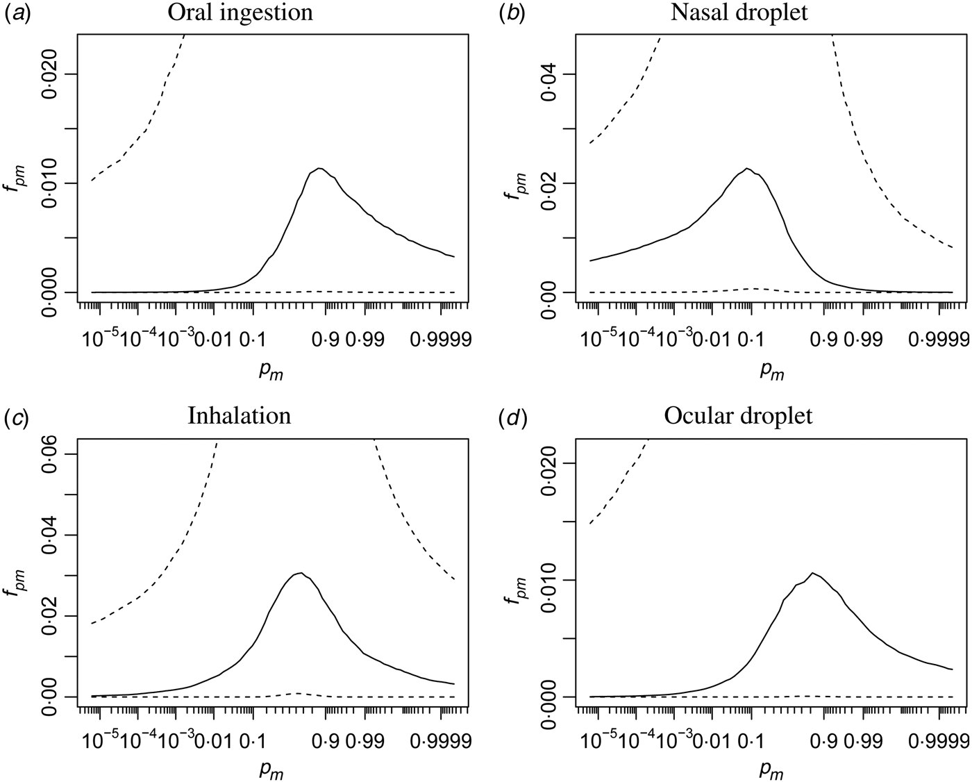
Fig. A1. Distributions of infectivities via the four different inoculation routes. Quantiles of the beta density (median, and 95% range) of the single-hit probability p m are shown, on a logit scale.
Parameter estimates for separate experiments
Table A1. Parameter estimates (mean and 95% range) for the separate adenovirus dose-response studies: infectivity (infection dose-response) parameters (α, β) and pathogenicity (conditional illness dose-response) parameters (η, r)
Separate experiments (Figs A2–A4)
Figures A2–A4 show infection dose-response, illness dose-response, and doses for 1% and 50% probability of infection and illness, respectively.
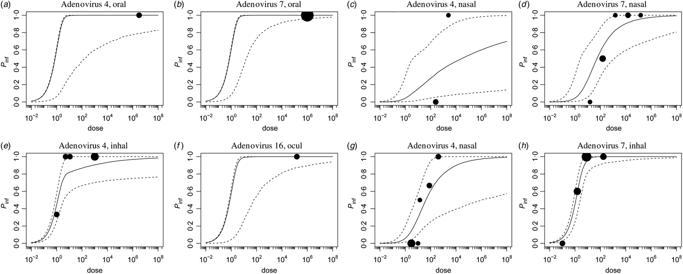
Fig. A2. Infection dose-response, separate studies.
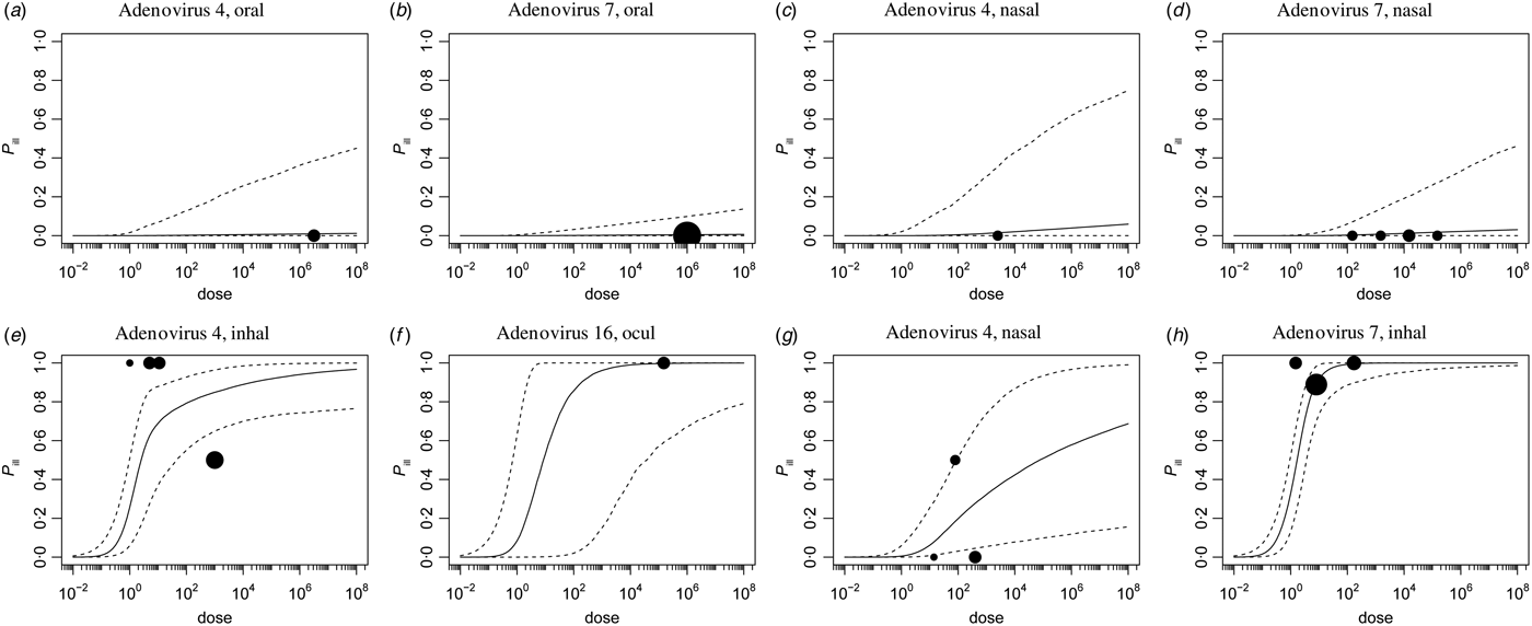
Fig. A3. Illness dose-response, separate studies.
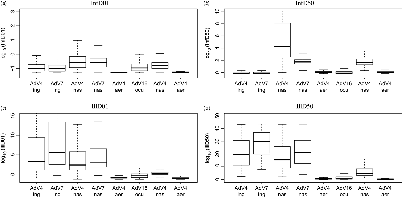
Fig. A4. Doses for 1% and 50% probability of infection and illness, for the separate studies.
Source code for the JAGS model
Posterior parameter samples were obtained using JAGS v. 4.2.0 [Reference Plummer27], controlled through rjags v. 4–5 [Reference Plummer28] in R v. 3.2.3 [29]. After a burn-in of 104 iterations, three chains were run in parallel, each with 106 iterations, and thinning 103, producing 3000 posterior samples of all parameters. Convergence was checked by Gelman and Geweke diagnostics (using the CODA package). Aside from the data (Table A1) that comprised eight experiments, four additional experiments were added, each consisting of only missing data, for each of the four exposure pathways. The parameters estimated for these four added experiments could be used for prediction, as these were sampled from the ‘group’ distributions for the four exposure pathways (because these consisted of missing data, not contributing to the likelihood in a Bayesian model).
Source code of the model is given below:
model {
# parent nodes: hyperparameters
for(k.study in 1:n.studies){
# infection (stage 1) and acute symptomatic illness (stage 2)
for (k.stage in 1:2){
mu.w [k.study,k.stage] <- mu.inoc.w [inoc [k.study],k.stage]
w [k.study,k.stage] ~ dnorm(mu.w [k.study,k.stage], 1/si.w [k.stage]ˆ2)
z [k.study,k.stage] ~ dnorm(mu.z [k.stage], 1/si.z [k.stage]ˆ2)
u [k.study,k.stage] <- exp(w [k.study,k.stage]) / (1+exp(w [k.study,k.stage]))
v [k.study,k.stage] <- exp(z [k.study,k.stage])
a [k.study,k.stage] <- u [k.study,k.stage]*v [k.study,k.stage]
b [k.study,k.stage] <- (1-u [k.study,k.stage])*v [k.study,k.stage]
}
for(k.dose in 1:n.doses [k.study]) {
# infection
num [k.study,k.dose] ~ dpois(volunt.data [k.study,k.dose,1])
gamma [k.study,k.dose] <- loggam(a [k.study,1] + b [k.study,1]) –
loggam(a [k.study,1] + b [k.study,1] + num [k.study,k.dose]) +
loggam(b [k.study,1] + num [k.study,k.dose]) - loggam(b [k.study,1])
prinf [k.study,k.dose] <- (1-exp(gamma [k.study,k.dose]))
volunt.data [k.study,k.dose,3] ~
dbin(prinf [k.study,k.dose],volunt.data [k.study,k.dose,2])
# acute symptomatic illness
prill [k.study,k.dose] <-
(1-pow(1 + b [k.study,2]*(volunt.data [k.study,k.dose,1]),-a [k.study,2]))
volunt.data [k.study,k.dose,4] ~ dbin(prinf [k.study,k.dose]*
prill [k.study,k.dose],volunt.data [k.study,k.dose,2])
}
}
for(k.inoc in 1:n.inoc){
for(k.stage in 1:2){
mu.inoc.w [k.inoc,k.stage] ~ dnorm(mu1.w [k.stage],1/si1.w [k.stage]ˆ2);
}
}
#
} # end model
ACKNOWLEDGEMENTS
This paper received no fnancial support.
DECLARATION OF INTEREST
None.


