


1. Introduction
While ideal flows (inviscid, with no heat conduction or additional energy dissipation effects; e.g. Landau & Lifshitz Reference Landau and Lifshitz1959) are an extreme limit, they play an important role in research, for example (i) as a basis for more realistic flows, with additional effects such as viscosity; (ii) for modelling the bulk of weakly interacting Bose–Einstein condensate superfluids, which can be approximated as an inviscid, compressible fluid with a polytropic index  $\gamma =2$; (iii) for modelling flow regimes which are not sensitive to the level of weak viscosity, such as in front of a round object; and (iv) for code validation and pedagogical reasons.
Janzen–Rayleigh expansions (JREs) can be broadly identified as an expansion of the flow variables in terms of the Mach number. JREs were used by Janzen (Reference Janzen1913) and Rayleigh (Reference Rayleigh1916) as a method to study the d'Alembert paradox with the addition of compressibility effects. They considered an inviscid, compressible, subsonic flow of a fluid with a polytropic equation of state (EoS), with no external forces or initial vorticity. Specifically, steady flow was assumed around a disk in two dimensions or around a sphere in three dimensions, with an incident uniform flow far from the body. Introducing the flow potential, a scalar nonlinear partial differential equation (PDE) was obtained, and expanded in the incident Mach number squared,  ${\mathcal {M}}_\infty ^{2}$.
Using the same set-up, the JRE was used to solve the flow around various blunt objects (Goldstein & Lighthill Reference Goldstein and Lighthill1944; Heaslet Reference Heaslet1944; Hasimoto Reference Hasimoto1951; Kawaguti Reference Kawaguti1951; Hida Reference Hida1953; Longhorn Reference Longhorn1954; Imai Reference Imai1957; Kaplan Reference Kaplan1957; Van Dyke Reference Van Dyke1958). The JRE has been generalized to several areas of research, such as vortex flows (e.g. Barsony-Nagy, Er-El & Yungster Reference Barsony-Nagy, Er-El and Yungster1987; Heister et al. Reference Heister, Mcdonough, Karagozian and Jenkins1990; Moore & Pullin Reference Moore and Pullin1991, Reference Moore and Pullin1998; Meiron, Moore & Pullin Reference Meiron, Moore and Pullin2000; Leppington Reference Leppington2006; Crowdy & Krishnamurthy Reference Crowdy and Krishnamurthy2018), porous channel flows (Majdalani Reference Majdalani2007; Maicke & Majdalani Reference Maicke and Majdalani2008, Reference Maicke and Majdalani2010; Cecil, Majdalani & Batterson Reference Cecil, Majdalani and Batterson2015), and acoustics (Slimon, Soteriou & Davis Reference Slimon, Soteriou and Davis2000; Moon Reference Moon2013) and could be used in a wide range of other applications, as we demonstrate below.
The two-dimensional (2-D) flow around a disk has been researched extensively (Janzen Reference Janzen1913; Rayleigh Reference Rayleigh1916; Van Dyke & Guttmann Reference Van Dyke and Guttmann1983; Guttmann & Thompson Reference Guttmann and Thompson1993), for example in search for a solution to the transonic controversy, namely, ‘the existence, or non-existence, of a continuous transonic flow, that is, without a shock wave, around a symmetrical wing profile, with zero incidence with respect to the undisturbed velocity’ (Ferrari Reference Ferrari1966). These and other problems that require a high-order expansion could not be explored as thoroughly in the 3-D case, because previous JREs for the sphere were limited to second, i.e.  ${\mathcal {M}}^{4}_\infty$, order (Kaplan Reference Kaplan1940; Tamada Reference Tamada1940). Indeed, a power series in the inverse radius
  $r^{-1}$ yields non-physical behaviour at the third, i.e.
  ${\mathcal {M}}^{6}_\infty$, expansion order. We avoid this supposed behaviour by showing that an additional power series emerges with radially logarithmic terms, allowing for JRE-based computations around a sphere to an arbitrary order. The resulting high-order 3-D expansions now facilitate a wide range of physical applications, including, for example, modelling the compressible flow in front of a sphere in order to model axisymmetric bodies in various fields of physics (e.g. Keshet & Naor Reference Keshet and Naor2016, and references therein), and exploring claims for an approximate universality among flows in front of such objects. Flows in higher dimensions,
  $d>3$, are also important, mainly for theoretical and pedagogical purposes, and similarly require logarithmic terms.
The paper is organized as follows. In § 2, we derive the JRE equations from the hydrodynamical ones. In § 3, we show that each term in the JRE of the flow potential around a hypersphere is a finite sum of a product of powers of the radial coordinate, powers of its logarithm and a set of orthogonal functions (Jacobi polynomials) of the polar coordinate. In § 4, we outline a semi-analytic algorithm to compute the JRE and a numerical pseudospectral method to solve the nonlinear compressible flow. We present the results of the semi-analytical JRE and the pseudospectral numerical solver, focusing in particular on the emergence of logarithmic JRE terms and compressibility effects, in § 5. The JRE is used to improve a hodograph approximation for the flow in front of the sphere in § 6. In § 7, we show that the axisymmetric flow in front of prolate spheroids is well approximated by that of the scaled flow in front of a sphere. We summarize and discuss our results in § 8. Appendix § A outlines the numerical solver, whereas the other supplementary material are available at https://doi.org/10.1017/jfm.2021.965 (OSM) and provide low-order JRE coefficients for flows around a disk and a sphere, and general results for the hodograph approximation.
A reader already familiar with the JRE may wish to skip its general derivation in § 2. A reader focused on the physical implications may wish to skip the mathematical section § 3 and the semi-analytic and numeric section § 4, and jump directly to the results in § 5. Sections §§ 6 and 7 demonstrate some applications of the JRE, and can be skipped if the reader is uninterested in the hodograph and prolate approximations.
2. Janzen–Rayleigh expansion
Consider an isentropic flow in  $d$ dimensions with no external forces of a perfect fluid with a polytopic, ideal gas EoS of adiabatic index
  $\gamma$,
 \begin{equation} p \propto {\rho ^{\gamma} } . \end{equation}
The equations governing the flow are the continuity equation,
 \begin{equation} \frac{{\partial \rho }}{{\partial t}} + \boldsymbol{\nabla} \boldsymbol{\cdot} ( {\rho \boldsymbol{u}} ) = 0 , \end{equation}
and the Euler equation,
 \begin{equation} \frac{{\partial {\boldsymbol{u}}}}{{\partial t}} + ({\boldsymbol{u}} \boldsymbol{\cdot} \boldsymbol{\nabla}) {\boldsymbol{u}} ={-} \frac{{\boldsymbol{\nabla} p}}{\rho } ={-}\frac{\boldsymbol{\nabla} c^{2}}{\gamma-1}. \end{equation}
Here,  $\rho, {\boldsymbol u}$ and
  $p$ are respectively the mass density, velocity and pressure,
  $c\equiv (\textrm {d} p/ \textrm {d} \rho )^{1/2}=(\gamma p/\rho )^{1/2}$ is the sound velocity and
  $\boldsymbol {\nabla }$ is the gradient operator in
  $d$ dimensions.
We henceforth assume steady flow. Combining (2.1) and (2.2) to eliminate  $\rho$ in favour of
  $c$ then yields
 \begin{equation} \frac{1}{\gamma-1}{\boldsymbol u} \boldsymbol{\cdot} \boldsymbol{\nabla} {c^{2}} ={-}{c^{2}}\boldsymbol{\nabla} \boldsymbol{\cdot} {\boldsymbol u} . \end{equation}
For our inviscid, steady flow, (2.3) yields the Bernoulli principle, namely, the quantity  $w{\boldsymbol {u}}^{2}+c^{2}$ is constant along streamlines, where we define
  $w\equiv (\gamma -1)/2$.
We consider the flow along a body for a uniform flow incident from infinity,
 \begin{equation} c( {r \to \infty } ) = {c_{\infty}} \quad \mbox{and}\quad {\boldsymbol{u}}( {r \to \infty } ) = u_{\infty}\hat{\boldsymbol z} , \end{equation}
where  $r$ is the radial coordinate,
  $z$ is the coordinates along the flow,
  $u=|\boldsymbol {u}|$ is the speed and the subscript
  $\infty$ indicates the far field region (tending to spatial infinity). Using the boundary conditions (2.5a,b) and the assumption that every streamline starts at infinity, the Bernoulli equation may be written as
 \begin{equation} w{{\boldsymbol u}^{2}} + c^{2} = w{{\boldsymbol u}_\infty ^{2}} + c_\infty ^{2} . \end{equation}
 Considering the subsonic regime, we restrict the discussion to a potential flow, writing the velocity as the gradient of the flow potential  $\phi$,
 \begin{equation} \boldsymbol{u} \equiv \boldsymbol{\nabla} \phi . \end{equation}
Isolating  $c^{2}$ from (2.6), substituting it into (2.4) and using the potential (2.7), we obtain a single PDE for the potential
  $\phi$ (Rayleigh Reference Rayleigh1916),
 \begin{equation} \tfrac{1}{2}(\boldsymbol{\nabla} \phi) \boldsymbol{\cdot} \boldsymbol{\nabla} {( {\boldsymbol{\nabla} \phi } )^{2}} = [ w {u_\infty ^{2}} + c_\infty ^{2} - w {{{( {\boldsymbol{\nabla} \phi } )}^{2}}} ]{\nabla^{2}}\phi . \end{equation}
We normalize the variables to obtain them in a dimensionless form, by taking  $\phi \to (u_{\infty }R)\phi$, and
  ${\boldsymbol r} \to R{\boldsymbol r}$ (which also normalize the velocity,
  ${\boldsymbol {u}}\to u_\infty {\boldsymbol {u}}$), where
  $R$ is a characteristic length scale, for example the radius of a hypersphere. Defining
  ${\mathcal {M}}_{\infty } \equiv u_{\infty }/c_{\infty }$ as the Mach number at infinity, we then arrive at the dimensionless equation
 \begin{equation} \tfrac{1}{2}(\boldsymbol{\nabla} \phi) \boldsymbol{\cdot} \boldsymbol{\nabla} {( {\boldsymbol{\nabla} \phi } )^{2}} = [ {w + {{\mathcal{M}}_\infty ^{{-}2}} - w{( {\boldsymbol{\nabla} \phi } )}^{2}}]{\nabla^{2}}\phi . \end{equation}
 We supplement this equation for the potential with two boundary conditions (BCs): the uniform incident flow from infinity, and the slip, no-penetration condition on the surface of the body ( ${\hat {\boldsymbol n}}\boldsymbol {\cdot } {\boldsymbol {u}}=0$), namely
 \begin{equation} \phi ( {r \to \infty } ) = z = r\cos \theta \quad\mbox{and}\quad \hat{\boldsymbol n}\boldsymbol{\cdot} \boldsymbol{\nabla} \phi = 0 . \end{equation}
Here,  $\hat {\boldsymbol n}$ is the normal to the body, and we use hyperspherical coordinates: a radial coordinate
  $0 \le r \le \infty$, a polar angle
  $0 \le \theta \le {\rm \pi}$ measured with respect to the uniform flow at infinity and
  $(d-2)$ additional angles. For axisymmetric flows such as in the case of a hypersphere, the flow is (by symmetry) independent of these additional angles.
To arrive at the JRE, we substitute the expansion
 \begin{equation} \phi{(\boldsymbol r)} \equiv \sum_{m = 0}^{\infty} {{\phi _m(\boldsymbol r)}{{\mathcal{M}}_{\infty}^{2m}}}, \end{equation}
into (2.9), and isolate the different powers of  ${\mathcal {M}}_\infty$. This leads to a recursive set of PDEs for
  $\phi _m$ (for
  $m \geq 1$),
 \begin{align} {\nabla^{2}}{\phi _m} & ={-} w{\nabla^{2}}{\phi _{m - 1}} \nonumber\\ & \quad +w \sum_{\{{m_1},{m_2},{m_3}\} = 0}^{m} {\delta_{{m_1} + {m_2} + {m_3},m - 1} ( {\boldsymbol{\nabla} {\phi _{{m_1}}} \boldsymbol{\cdot} \boldsymbol{\nabla} {\phi _{{m_2}}}} ){\nabla^{2}}{\phi _{{m_3}}}} \nonumber\\ & \quad +\frac{1}{2} \sum_{\{{m_1},{m_2},{m_3}\} = 0}^{m} {\delta_{{m_1} + {m_2} + {m_3},m - 1} \boldsymbol{\nabla} ( {\boldsymbol{\nabla} {\phi _{{m_1}}} \boldsymbol{\cdot} \boldsymbol{\nabla} {\phi _{{m_2}}}} ) \boldsymbol{\cdot} \boldsymbol{\nabla} {\phi _{{m_3}}}}, \end{align}
with an initial equation
 \begin{equation} {\nabla^{2}}{\phi _0} = 0, \end{equation}
along with BCs
 \begin{equation} {\phi _m}( {r \to \infty } ) = {\delta _{m,0}} r\cos \theta, \end{equation}
at infinity, and
 \begin{equation} {\hat{\boldsymbol n}} \boldsymbol{\cdot} \boldsymbol{\nabla} {\phi _m} = 0, \end{equation}
on the body. Here,  $\delta _{i,j}$ is the Kronecker delta symbol.
The zeroth-order (2.13) is the Laplace equation for  $\phi _0$, corresponding to the incompressible limit
  ${\mathcal {M}}_\infty \to 0$. For higher orders, (2.12) can be regarded as a set of Poisson equations for
  $\phi _m$ at each order
  $m$, with a source term being a function of the lower-order solutions,
  $\{\phi _i\}^{m-1}_{i=0}$, and their derivatives. In general, the solution to (2.12) at any order
  $m\geq 1$ under the BCs (2.14) and (2.15) is a sum of an inhomogeneous solution and a homogeneous solution,
 \begin{equation} \phi_m = \phi_m^{{(in)}} + \phi_m^{{(ho)}}, \end{equation}
where  $\phi _m^{{(ho)}}$ solves the Laplace equation.
The JRE (2.11) is constructed by iteratively determining the functions  $\phi _m$. One starts by deriving
  $\phi _0$, obtained as the solution to the zeroth-order Laplace equation (2.13) under the BCs. Increasingly higher-order functions
  $\phi _m$ are then incrementally derived, by solving the corresponding Poisson equations (2.12) under the same BCs. At each order
  $m\geq 1$, the inhomogeneous solution
  $\phi _m^{{(in)}}$ is fixed by the source term in the corresponding (2.12), which is explicitly written once all lower-order functions
  $\phi _m$ are determined. This solution is then combined with an expansion
  $\phi _m^{{(ho)}}$ of homogenous solutions, the coefficients of which are determined by applying the BCs to the resulting (2.16).
3. JRE for a hypersphere
Simple solutions exist for the flow around a  $d$-dimensional hypersphere, for which the Laplace equation has known analytic solutions, and the Poisson equation is easily solved. Choosing the characteristic length
  $R$ as the hypersphere radius, the normalized no-penetration BC (2.15) here simplifies to
 \begin{equation} \partial_r\phi(r=1,\theta) = 0. \end{equation}
Considering the hyperspherical and axial symmetries, it is useful to write the general solution to the Laplace equation (2.13) as an infinite sum of positive and negative radial powers (e.g. Feng, Huang & Yang Reference Feng, Huang and Yang2011)
 \begin{equation} \sum_{n = 1}^{\infty} {(A_n r^{n}+B_n r^{ - n - d + 2}){\mathcal{J}}_n^{(d)}(\mu)}, \end{equation}
where we define  $\mu \equiv \cos \theta$, the normalized Jacobi polynomials
 \begin{equation} {\mathcal{J}}_n^{(d)}( {\mu } ) \equiv \frac{{J_n^{( {({{d - 3}})/{2},({{d - 3}})/{2}} )}( {\mu } )}}{{J_n^{( {({{d - 3}})/{2},({{d - 3}})/{2}} )}( 1 )}} = \frac{C_n^{({d}/{2}-1)}(\mu)}{{{n+d-3}\choose {n}}} , \end{equation}
and numerical coefficients  $A_n$ and
  $B_n$. Here,
  $J_n^{(\alpha,\beta )}(\mu )$ and
  $C_n^{(\alpha )}(\mu )$ are respectively the standard Jacobi and Gegenbauer polynomials.
The source term in (2.12) is a sum of multiple terms, each composed of even derivatives in  $\theta$ and odd multiples of functions
  $\phi$. Therefore, the polar dependence will always exhibit the same symmetry as the zero-order solution
  $\phi _0$. As the hypersphere is isotropic, the incompressible flow also shows a backward–forward symmetry. We conclude that the functions
  ${\mathcal {J}}_n^{(d)}$ appearing in
  $\phi _m$ at all orders
  $m$ have only odd
  $n$. Next, we construct the hypersphere JRE by considering increasingly larger orders
  $m$.
$m$.
3.1. Zeroth order:  $m=0$
$m=0$

For the  $m=0$ order, the infinity BC (2.14) allows only the radially linear and decaying terms in the solution (3.2). The no-penetration BC (3.1) restricts the solution further, allowing for only the decaying term proportional to
  ${\mathcal {J}}_1^{(d)}(\mu ) = \mu$. The solution to the Laplace equation (2.13) around a
  $d$-dimensional hypersphere thus becomes
 \begin{equation} \phi _0^{(d)}(r,\theta) = \left[ {r + \frac{1}{{( {d - 1} ){r^{d - 1}}}}} \right]\cos\theta. \end{equation}
Henceforth, we omit the dimension superscript  $(d)$ unless necessary.
3.2. First order: $m=1$

The first-order potential,  $\phi _1$, is determined by
 \begin{equation} {\nabla^{2}}{\phi _1} ={-} w{\nabla^{2}}{\phi _{0}} +\tfrac{1}{2} ( \boldsymbol{\nabla} {\phi _{{0}}} ) \boldsymbol{\cdot} \boldsymbol{\nabla} ( \boldsymbol{\nabla} {\phi _{{0}}} )^{2} +w ( \boldsymbol{\nabla} {\phi _{{0}}} )^{2}{\nabla^{2}}{\phi _{0}}, \end{equation}
which, by the zeroth-order (2.13), simplifies to
 \begin{equation} {\nabla^{2}}{\phi _1} = \tfrac{1}{2} ( \boldsymbol{\nabla} {\phi _{{0}}} ) \boldsymbol{\cdot} \boldsymbol{\nabla} ( \boldsymbol{\nabla} {\phi _{{0}}} )^{2}. \end{equation}
Plugging the  $m=0$ solution (3.4) into (3.6) gives the Poisson equation with the explicit source term,
 \begin{align} {\nabla^{2}}{\phi _1} & = [{-}3\mu\!+\!(2+d)\mu^{3}]r^{{-}d-1}\frac{d }{d-1} + [({-}3+d)\mu\!+\!(2\!+\!d-d^{2})\mu^{3}]r^{{-}2d-1}\frac{2d}{(d-1)^{2}} \nonumber\\ & \quad +[({-}3+2d)\mu+(2+d-3d^{2}+d^{3})\mu^{3}]r^{{-}3d-1}\frac{d}{(d-1)^{3}} . \end{align}
The orthogonal decomposition of Jacobi polynomials (Chaggara & Koepf Reference Chaggara and Koepf2010) then yields
 \begin{align} {\nabla^{2}}{\phi _1} & = {\mathcal{J}}_3( {\mu } )r^{{-}d-1} d \nonumber\\ &\quad + [{-}2d {\mathcal{J}}_1( {\mu } ) -(1+d) (d-2){\mathcal{J}}_3( {\mu } )] r^{{-}2d-1} \frac{2d }{(d-1) (d+2)} \nonumber\\ &\quad + [d({-}4+3d) {\mathcal{J}}_1( {\mu } ) - (1+d-d^{2})(d-2){\mathcal{J}}_3( {\mu } )] r^{{-}3d-1} \frac{d}{(d-1)^{2}(d+2)} . \end{align}
This result may be compactly written in the form
 \begin{equation} {\nabla^{2}}\phi_1 = \sum_{k,n} {s^{({in})}_{1,k,n}{r^{k}}{\mathcal{J}}_n( {\mu } )} , \end{equation}
where  $s^{({in})}_{m,k,n}$ are the expansion coefficients of the order-
 $m$ Poisson source term, for radial order
  $k$ and angular order
  $n$; these coefficients are directly read off the right-hand side of (3.8). The OSM provides these and other coefficients explicitly, for
  $d=2$ and
  $d=3$ (tables 1-3 therein).
As the Poisson equation is linear, it suffices to solve, for arbitrary  $k$ and
  $n$, the equation
 \begin{equation} {\nabla^{2}}\phi_{k,n} = {r^{k}}{\mathcal{J}}_n( {\mu } ) . \end{equation}
This equation has the particular solution
 \begin{equation} \phi _{k,n}^{({in})} = \frac{{{r^{k+2}}{\mathcal{J}}_n( {\mu })}}{{(k+2) ( {k + d} ) - n( {n + d - 2} )}} , \end{equation}
provided that  $k \notin \{- d - n, n-2\}$. These two exceptional values of
  $k$ do not occur at order
  $m=1$, as seen from (3.8), but they may appear at higher orders, as discussed below in § 3.3. We may now expand the inhomogeneous solution as
 \begin{equation} \phi^{{(in)}}_1 = \sum_{k,n}{s^{({in})}_{1,k,n}\phi^{{(in)}}_{k,n}} , \end{equation}
where the numerical coefficients  $s^{({in})}_{1,k,n}$ are determined by equating (3.8) and (3.9).
From (3.8) and (3.11), we see that the largest (i.e. least negative) power of  $r$ for
  $m=1$ is
  $k_{max}=-d+1<0$, implying that
  $\phi ^{{(in)}}_1$ includes only radially decaying terms. For higher orders, (2.12) combines the derivatives of multiple
  $\phi _m$ functions, but the highest radial power
  $k_{max}$ in the source term remains no larger than
  $-d-1$. Consequently, the inhomogeneous solution for all
  $m\geq 1$ orders includes only radially decaying terms. This conclusion, combined with the BCs, indicates that the homogeneous solution may be expanded with only negative powers of
  $r$ for any
  $m>0$,
 \begin{equation} \phi^{{(ho)}}_{m>0} = \sum_{n = 1}^{\infty} {s^{(ho)}_{m,n} {r^{ - n - d + 2}}{\mathcal{J}}_n(\mu)} , \end{equation}
where  $s^{(ho)}_{m,n}$ are numerical coefficients, to be determined below.
The full solution for  $m=1$ now becomes
 \begin{equation} \phi_1 = \phi_1^{{(in)}} + \phi_1^{{(ho)}} = \sum_{k,n}{s_{1,k,n} r^{k} {\mathcal{J}}_n(\mu)}, \end{equation}
where we have introduced the combined numerical coefficients
 \begin{equation} s_{1,k,n}=\frac{s^{({in})}_{1,k-2,n}}{k(k+d-2)-n(n+d-2)}+s^{(ho)}_{1,n}\delta_{k,-n-d+2} . \end{equation}
These coefficients may now be determined from the no-penetration BC (3.1),
 \begin{equation} \frac{\partial \phi_1}{\partial r}(r=1) = \sum_{k,n}{k s_{1,k,n} {\mathcal{J}}_n(\mu)} = 0, \end{equation}
implying that
 \begin{equation} s^{(ho)}_{1,n} = \frac{1}{n+d-2} \sum_{k,n}{\frac{k s^{({in})}_{1,k-2,n}}{k(k+d-2)-n(n+d-2)}}. \end{equation}
As the coefficients  $s^{({in})}_{1,k,n}$ are known from (3.8) and (3.9), the solution (3.14) is completely specified by (3.15) and (3.17).
3.3. Higher orders: $m\geq 2$

Substituting  $\phi _0$ and
  $\phi _1$ in the Poisson equation (2.12) for the next
  $m=2$ order results again in an equation of the form (3.9), but now for
  $\phi _2$ and with different coefficients. Equations of the same form persist for higher orders
  $m$, as long as the source term in (2.12) is free of non-zero terms
  $s_{m,k,n}$ which satisfy one of the aforementioned special conditions,
  $k=- d - n$ or
  $k=n-2$. Indeed, the source term consists of differential operators of the form
  $\nabla ^{2}f(r,\mu )$ and
  $\boldsymbol {\nabla } f(r,\mu )\cdot \boldsymbol {\nabla } g(r,\mu )$, where
  $f$ and
  $g$ are constructed from lower-order
  $\phi$ terms. As long as
  $f$ and
  $g$ are sums of terms, each of which is a product of powers of
  $r$ and Jacobi polynomials in
  $\mu$, the source term remains of the form (3.9).
For the special cases  $k \in \{- d - n, n-2\}$, the solution to (3.10) is no longer given by (3.11), which formally diverges as its denominator vanishes. It is sufficient to consider the former case,
  $k=-d-n$, as the latter,
  $k = n -2$, is then obtained by the transformation
  $n \to - n - d + 2$, under which
  ${\mathcal {J}}_n^{(d)}$ remains invariant. Here, the inhomogeneous solution to (3.10) becomes
 \begin{equation} \phi_{k={-}d-n,n} ={-}\frac{{\varGamma [ {2,( {2n + d - 2} )\ln ( r )} ]}}{{{{( {2n + d - 2} )}^{2}}}} {r^{n}} {\mathcal{J}}_n( {\mu } ) , \end{equation}
where  $\varGamma (\xi,\eta )$ is the incomplete gamma function, defined by
 \begin{equation} \varGamma ( {\xi,\eta} ) = \int_\eta^{\infty} {{t^{\xi - 1}}{\textrm{e}^{ - t}}\, \textrm{d} t} . \end{equation}
 Once a logarithmic term from (3.18) appears in the inhomogeneous solution for  $\phi _m$, as a result of a special
  $k$ term in the source-term expansion (3.9), a power series in
  $r$ as in (3.14) is no longer sufficient. Indeed, when
  $\xi =\ell +1$ and
  $\eta =\tau \ln (r)$ for integers
  $\ell$ and
  $\tau$,
 \begin{equation} \varGamma [ {\ell + 1,\tau\ln (r)} ] = \frac{{\ell!}}{{{r^{\tau}}}}\sum_{j = 0}^{\ell} {\frac{{{{[\tau\ln (r) ]}^{j}}}}{{j!}}}, \end{equation}
contains logarithmic, and not only polynomial, radial terms. Since  $\ln (r)$ cannot be expanded as a power series of
  $r^{-1}$ valid over the full
  $1\leq r<\infty$ range, one must then take into account logarithmic terms in the expansion of
  $\phi _m$ and in the resulting source terms of higher-order functions.
Generalizing the prototypical source term in (3.9) to include a logarithm of  $r$ to some power
  $\ell$, we must therefore also consider the generalized equation
 \begin{equation} {\nabla^{2}}\phi_{k,n,\ell} = r^{k} {\mathcal{J}}_n( {\mu } ) \ln^{\ell}(r). \end{equation}
As long as  $k, d$, and
  $n$ do not satisfy one of the special cases
 \begin{equation} k \in \{ - d - n, n-2\} , \end{equation}
the inhomogeneous solution to this equation is
 \begin{align} \phi_{k,n,\ell} & = \frac{{{\mathcal{J}}_n( {\mu } )}}{{2n + d - 2}} \left({r^{{-}n-d+2}}\frac{{\varGamma [ {\ell + 1, ( {-d - k - n } )\ln (r)} ]}}{{{{( { - d - k - n} )}^{\ell + 1}}}}\right. \nonumber\\ &\quad \left. - {r^{n}}\frac{{\varGamma [ {\ell + 1,( { n - k -2} )\ln (r)} ]}}{{{{({ n - k-2} )}^{\ell + 1}}}} \right) , \end{align}
whereas for  $k=-d-n$ we find
 \begin{equation} \phi _{k={-} d - n,n,\ell} ={-} {r^{n}}{\mathcal{J}}_n( {\mu } ) \frac{{\varGamma[ {\ell + 2,( {2n + d - 2} )\ln (r)} ]}}{{{{(\ell + 1)( {2n + d - 2} )}^{\ell + 2}}}} . \end{equation}
The case  $k=n-2$ is again obtained using the transformation
  $n \to - n - d + 2$,
 \begin{equation} \phi _{k={-}n-d+2,n,\ell} ={-} {r^{{-}n-d+2}}{\mathcal{J}}_{n} ( {\mu } )\frac{{\varGamma[ {\ell + 2,( {-2n-d+2} )\ln (r)} ]}}{{{{(\ell + 1)( {-2n-d+2} )}^{\ell + 2}}}} . \end{equation}
 The overall solution for  $\phi _m$ may now be expanded as the finite sum
 \begin{equation} \phi_m = \sum_{k,n,\ell}{s_{m,k,n,\ell} r^{k}{\mathcal{J}}_n^{(d)}( {\mu } )\ln^{\ell} (r)}, \end{equation}
where the numerical coefficients  $s_{m,k,n,\ell }$ are determined using the BCs in analogy with the above
  $m=2$ discussion. The expansion (3.26) is complete, as the inhomogeneous solution yields only powers of
  $r$ and
  $\ln (r)$, and the homogeneous solution yields only powers of
  $r$, so the resulting higher-order source terms are again of the form (3.21).
One can prove, by induction, the following rules for the  $m\geq 1$ indices in (3.26),
 \begin{equation} 1-d-2md \leq k \leq 1-d, \end{equation}
and
 \begin{equation} 1\leq n \leq 1+2m. \end{equation}
Logarithmic terms, if they emerge, are limited to indices
 \begin{equation} 0\leq \ell \leq m, \end{equation}
because combining the particular solutions (3.24) and (3.25) with the property of the incomplete gamma function (3.20) shows that the highest logarithmic power increases at most by one in each JRE order (Imai Reference Imai1942, which considered only 2-D flows). Additional rules for the logarithmic term are discussed in § 5.
4. Semi-analytical and numerical solvers for disk and sphere flows
We explicitly solve (2.12) analytically and using a computer-aided symbolic algebra program (Wolfram Mathematica; Wolfram, Research Inc 2019; a notebook is provided at https://physics.bgu.ac.il/~wallersh/) for the hypersphere in the  $d=2$ and
  $d=3$ cases; namely, we derive the flows around a 2-D disk and around a 3-D sphere. The normalized Jacobi functions reduce to Chebyshev polynomials
  ${T_n}$ in two dimensions,
 \begin{equation} {\mathcal{J}}_n^{(2)}( {\cos \theta } ) = {T_n}( {\cos \theta } ) = \cos ( {n\theta } ) , \end{equation}
and to Legendre polynomials  ${P_n}$ in three dimensions,
 \begin{equation} {\mathcal{J}}_n^{(3)}( {\cos \theta } ) = {P_n}( {\cos \theta } ) . \end{equation}
As discussed in § 3, we consider the generalized expansion (2.11) and (3.26) of the flow potential in each case,
 \begin{equation} \phi^{{disk}} = \left(r+\frac{1}{r}\right) \cos\theta + \sum_{m=1}^{\infty} {\sum_{\ell=0}^{m} {\sum_{n=1}^{2m+1} {\sum_{k={-}1-4m}^{{-}1} {a_{m,k,n,\ell}{{\mathcal{M}}_\infty^{2m}}{r^{k}}\cos ( {n\theta } ){{\ln }^{\ell}}(r)}}}}, \end{equation}
and
 \begin{equation} \phi^{{sphere}} =\left(r+\frac{1}{2r^{2}}\right) \mu + \sum_{m=1}^{\infty} {\sum_{\ell=0}^{m} {\sum_{n=1}^{2m+1} {\sum_{k={-}2-6m}^{{-}2} {{b_{m,k,n,\ell}}{{\mathcal{M}}_\infty^{2m}}{r^{k}}{P_{n}}(\mu){{\ln }^{\ell}}(r)}}}} , \end{equation}
where  $a$ and
  $b$ are the expansion coefficients in two and three dimensions, respectively, and the summation index
  $n$ takes only odd values.
We compute these JREs analytically, following the steps outlined in § 3. The  $m=0$ term is given by (3.4). For each order
  $m>0$, we compute the source terms on the right-hand side of (2.12), and decompose them into a sum of terms proportional to
  $r^{k} {\mathcal {J}}_n( {\mu } ) \ln ^{\ell }(r)$ as in (3.21). The inhomogeneous solution
  $\phi ^{{(in)}}_m$ is then obtained as the corresponding sum of solutions of the form (3.23)–(3.25), and added to the homogeneous solution
  $\phi ^{{(ho)}}_m$ of (3.13). The coefficients
  ${s^{(ho)}_{m,n}}$ in the latter sum are determined from the no-penetration BC, as demonstrated for
  $m=1$ in (3.17). This process is repeated until the designated order of the JRE is reached.
The JRE results are also compared with the flow obtained from a numerical solution to the nonlinear equation (2.9). We follow Pham, Nore & Brachet (Reference Pham, Nore and Brachet2005) and use a pseudospectral collocation method (Boyd Reference Boyd2001) for a fast numerical convergence. In the pseudospectral method, the solution to a PDE is expanded in terms of basis functions, each being a product of individual (and typically orthogonal) functions for each coordinate. In collocation methods, the PDE is then evaluated and solved at a set of points, usually taken as the roots of the basis functions. This leads to a set of linear equations for the basis function coefficients, which are solved to give an approximate PDE solution. In general for pseudospectral methods, if the solution is smooth (all derivatives of all orders are continuous) then the convergence is exponential in the number  $N$ of collocation points (Boyd Reference Boyd2001),
  $O(\textrm {e}^{-N})$.
Pham et al. (Reference Pham, Nore and Brachet2005) use the Chebyshev–Fourier set of basis functions, with  $\cos (n\theta )$ and
  $\sin (n\theta )$ with integer
  $n$ as angular basis functions. As discussed in § 3, the analytical solution for
  $\phi$ is a sum of
  $\cos (n\theta )$ terms with odd positive
  $n$, so we expand the flow potential in odd cosine functions. To achieve the same accuracy as Pham et al. (Reference Pham, Nore and Brachet2005), we need only a fourth of the angular basis functions.
For the radial part, we apply an inversion map  $\varrho \equiv r^{-1}$ and expand in Chebyshev polynomials
  $T_k(\varrho )$, to resolve both small and large
  $r$ behaviour. The pseudospectral expansion thus becomes
 \begin{equation} {\phi _{{ps}}} = \phi_0 + \sum_{k=0}^{k_{\max}}\sum_{n=0}^{n_{\max}} {{c_{k,n}}{T_k}(\varrho)\cos [ {( {2n + 1} )\theta } ]}. \end{equation}
Here,  $k_{max}+1$ and
  $n_{max}+1$ are the radial and angular resolution, i.e. the number of collocation points, and
  $c_{k,n}$ are real coefficients. The BCs for
  $\phi _{ps}$ are guaranteed by offsetting collocation points from the boundaries and picking a potential
  $\phi _0$ consistent with the BCs; a simple choice is the incompressible solution (3.4). Since the effective computational domain and symmetry are the same in our 2-D and 3-D frameworks, we expand both flows, around a disk and around a sphere, in the same basis functions (4.5). Appendix § A provides more details on the calculations of
  $c_{k,n}$ and shows the numerical convergence.
5. Results
We calculate the JRE (4.3) and (4.4) up to order  $m=30$ for the disk and
  $m=18$ for the sphere. We provide explicit expressions for the coefficients
  $a$ and
  $b$ up to order
  $m=3$ (i.e.
  ${\mathcal {M}}_\infty ^{6}$) for a general
  $\gamma$ in the OSM (tables 1-3). For the pseudospectral code, we use a resolution up to 32 Chebyshev and 64 odd cosine functions, but as shown below, much lower orders and resolutions are sufficient to capture the behaviour of the flow with high accuracy even for maximal compressibility (see figure 2 and 6). The results are presented in the following figures mainly for
  $\gamma =7/5$. Different choices of
  $\gamma$ give qualitatively similar results, as demonstrated for
  $\gamma =5/3$ in figure 3(b).
Figure 1 shows the flow around a disk (a) and a sphere (b) for incident Mach numbers at infinity approaching the respective critical (i.e. sonic) Mach numbers. The latter are tuned to yield a sonic flow at the equator of the hypersphere,  ${\mathcal {M}}(r=1,\theta ={\rm \pi} /2)=1$, leading to
  ${\mathcal {M}}^{{disk}}_c \simeq 0.3982$ in two dimensions and
  ${\mathcal {M}}^{{sphere}}_c \simeq 0.5619$ in three dimensions. We compute the critical Mach number
  ${\mathcal {M}}_\infty ={\mathcal {M}}_{cr}$ by substituting
  ${\mathcal {M}}=1$ in the Bernoulli equation and solving the resulting implicit equation
 \begin{equation} \frac{u( {{\mathcal{M}}_{cr}} )^{2}}{u_\infty^{2}} = \frac{{w + {\mathcal{M}}_{cr} ^{ - 2}}}{{w + 1}}, \end{equation}
where  $u$ is evaluated at the equator, using a high-order JRE.

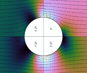
Figure 1. JRE solution to the critical flow around a unit hypersphere (white disk) for  $\gamma =7/5$ in two dimensions (a unit disk; (a); incident near-critical Mach number
  ${\mathcal {M}}_\infty ={\mathcal {M}}^{{disk}}_c \simeq 0.3982$) and three dimensions (a unit sphere; (b);
  ${\mathcal {M}}^{{sphere}}_c \simeq 0.5619$). In such a critical flow, the Mach number at the equator of the body locally reaches
  ${\mathcal {M}}_{{eq}}=1$. Streamlines (arrows) represent the trajectory of the flow (passing through equidistant points at
  $z=\pm 2$ (black dots). The normalized (dimensionless) speed
  $|u|$ is computed up to different JRE orders
  $m$ (of
  ${\mathcal {M}}_\infty ^{2}$ in (2.11); see labels) in each quadrant. The effect of compressibility is particularly noticeable by comparing the
  $m=0$ and
  $m=5$ approximations along the
  $x>0$ axis.
The colour intensity (cubehelix; Green Reference Green2011) in the figure represents the normalized speed  $|u|$. The flow is symmetric under both
  $x$ and
  $z$ reflections, i.e.
  $\theta \to -\theta$ and
  $\theta \to {\rm \pi}-\theta$, so it is sufficient to plot only one quadrant of the
  $x-z$ plane. We thus utilize all four quadrants to show the differences between the JRE obtained up to different,
  $m=0$ to
  $m=5$, orders (see labels). To show the JRE corrections to the flow, we plot the streamlines (arrows) that pass through a set of fixed equidistant points at
  $z=\pm 2$, so the differences between quadrant arrows are meaningful. Comparing the different quadrants shows that the compressible effects captured by higher orders
  $m$ raise the velocity and lower the density in the equatorial plane (notice the misaligned streamlines and mismatched colours along the
  $z=0, x>1$ line).
Figure 2 shows the compressible contribution to the flow around a sphere; qualitatively similar results are obtained for the disk. The contribution is computed based on JREs of different orders, as well as on the numerical solution, and shown for the polar velocity on the sphere (column a), the polar velocity at the equatorial plane (column b) and the radial velocity along the symmetry axis (column c). We plot these profiles for two different flows, with incident Mach numbers  ${\mathcal {M}}_\infty =0.1$ to demonstrate a subsonic case (row 1), and
  ${\mathcal {M}}_\infty ={\mathcal {M}}_c\simeq 0.5619$ for the critical case (row 2). As seen from row 1, at low Mach numbers, the JRE converges rapidly: the
  $m=1$ JRE is sufficient to accurately (within
  $\sim 0.005\,\%$ in
  $\boldsymbol {u}$ for
  ${\mathcal {M}}_\infty =0.1$) capture the compressible effects. Convergence is slower for larger
  ${\mathcal {M}}_\infty$, with high orders needed to obtain an accuracy sufficient for precision applications (compressible effects captured within
  $\sim 5\,\%$ in
  ${\boldsymbol {u}}$ for
  $m=1$) and delicate questions (such as the transonic controversy) in the critical limit.

Figure 2. Compressible corrections to the flow around a 3-D sphere for  $\gamma =7/5$ according to different JRE orders and to the pseudospectral (ps,
  $8\times 8$ resolution) solver (see legend). Profiles are shown for the flow along the longitude of the sphere (column a), at different radii above the equator (column b) and along the symmetry axis (column c), for both a subsonic flow with
  ${\mathcal {M}}_\infty =0.1$ (row 1) and for the critical flow (row 2).
For the flow around a disk in two dimensions, we find no logarithmic ( $\ln r$) terms in the flow potential, for any
  $\gamma$. Namely, all computed JRE (4.3) coefficients
  $a$ with
  $\ell \neq 0$ vanish, as illustrated in table 1 in the OSM up to order
  $m=3$. We confirm this behaviour for arbitrary
  $\gamma$ up to order
  $m=30$. Using a prescribed
  $\gamma$ speeds up the JRE computations, allowing us to reach higher orders. We thus compute the JRE up to order
  $m=50$ for the specific cases
  $\gamma \in \{1, 7/5, 5/3, 2\}$, corresponding respectively to isothermal, ideal diatomic, ideal monatomic and weakly interacting Bose, gasses. In all of these cases, we find no logarithmic terms in the flow potential.
In contrast, logarithmic terms are unavoidable in the flow around a sphere in three dimensions, for any  $\gamma$. Indeed, the JRE (4.4) shows the first logarithmic term at order
  $m=3$, for
  $k=-8, n=7$ and
  $\ell =1$, as indicated in table 3 in the OSM. This is proportional to
  $5+7\gamma +2\gamma ^{2}$, which vanishes only for negative, non-physical
  $\gamma$ values. In addition to such
  $\ell =1$ terms for all orders
  $m\geq 3$, we find
  $\ell =2$ terms for all orders
  $m\geq 6, \ell =3$ terms for all orders
  $m\geq 9$, and so on, with the highest logarithmic term order increasing by one every three orders in
  $m$. Furthermore, the term with the highest logarithm power is also proportional to
  $\propto {r^{-2m-2}P_{2m+1}(\mu )}$. This behaviour is verified up to order
  $m=18$ for arbitrary
  $\gamma >-1$, and up to order
  $m=30$ for the specific values of
  $\gamma$ chosen above.
While proving that these effects persist as  $m$ increases to infinity is beyond the scope of the present work, we hypothesize that they do:
Conjecture 5.1 Logarithmic JRE terms never appear in the flow of a polytropic  $\gamma \geq 1$ fluid around a disk.
Conjecture 5.2 For the flow around a sphere, the highest  $\ell$ of JRE terms
  $\propto {{\mathcal {M}}_\infty ^{2m}}{{\ln }^{\ell }(r)}$ is
  $\ell _{max}=\lfloor m/3 \rfloor$.
6. Example: an improved axial hodograph approximation
The flow in front of a blunt body has important implications in diverse physical applications, and is well approximated in both subsonic and supersonic regimes by expanding the perpendicular gradients  $q\equiv \partial _\theta u_\theta |_{\theta =0}$ in terms of the parallel (normalized) velocity
  $u=|u_r|$ (Keshet & Naor Reference Keshet and Naor2016). In the subsonic regime of this hodograph approximation,
  $q=q(u)$ is defined in the
  $0< u<1$ region between the stagnation point and spatial infinity, and is expanded around the stagnation point in the form
  $q(u) \approx q_0+q_1u+q_2u^{2}+q_3u^{3}$, which we designate as a third-order hodograph approximation, Hodo(3). It can be shown that
  $q_0$ does not vary much with respect to the incompressible case,
  $q_1=-1/2$, and
  $q_2$ is small with respect to
  $q_3$ (Keshet & Naor Reference Keshet and Naor2016).
Using the JRE for the sphere, here we calculate the coefficients  $q_i$ analytically, for given order
  $m$. The resulting expressions for the coefficients are provided for
  $1\leq m\leq 4$, as a function
  ${\mathcal {M}}_\infty$ and
  $\gamma$, in table 4 in the OSM. For illustration, table 1 provides the numerical values of these coefficients for the critical Mach number with
  $\gamma =7/5$. The coefficients converge rapidly, reaching three-digit accuracy for
  $m=4$. The effect of compressibility can be seen to be small, as
  $q_2$ and
  $q_3$ are smaller than
  $q_0$ and
  $q_1$ by two orders of magnitude. We verify the small deviation of
  $q_0$ from its incompressible value
  $3/2$, the precise result
  $q_1=-1/2$ for all orders, and that
  $q_2\approx q_3/3$ is small albeit non-negligible.
Table 1. Coefficients of the first four terms in the Taylor expansion of  $q(u)$, for different JRE orders
  $m$, at the critical Mach number
  ${\mathcal {M}}_\infty ={\mathcal {M}}_{\infty }\simeq 0.5619$ for the flow of a
  $\gamma =7/5$ fluid around a sphere. See the OSM, appendix B for analytic expressions for
  $q$ with arbitrary
  ${\mathcal {M}}_\infty$ and
  $\gamma$.

Figure 3 shows the compressible contribution to the radial velocity along the symmetry axis of a sphere, with and without the JRE corrections, for a flow at the critical Mach number. Results are shown for both  $\gamma =7/5$ (a) and
  $\gamma =5/3$ (b). The two panels slightly differ because they pertain to different
  ${\mathcal {M}}_\infty$ values; for the same
  ${\mathcal {M}}_\infty$, the axial flow for different
  $1<\gamma <2$ values are nearly indistinguishable. The corrected hodograph approximation provides a much better fit to the JRE and to the actual flow; an advantage of this approximations is its smooth transition into the supersonic regime (Keshet & Naor Reference Keshet and Naor2016).

Figure 3. Compressibility contribution to the velocity along the symmetry axis of a sphere near the critical Mach number, for  $\gamma =7/5$ ((a)
  ${\mathcal {M}}_\infty ={\mathcal {M}}_c\simeq 0.5619$) and
  $\gamma =5/3$ (b)
  ${\mathcal {M}}_\infty ={\mathcal {M}}_c\simeq 0.5462$). Results shown for a numerically converged pseudospectral calculation (ps,
  $8\times 8$ resolution, solid black curve), a first-order JRE (JRE(1), dot-dashed red) and second-order (JRE(2), dot-dash-dashed cyan) and hodograph approximations with (Hodo(4), dotted blue) and without (Hodo(3), dashed green) the
  $q_2$ coefficient.
7. Example: an approximately universal flow in front of spheroids
It has been suggested (Keshet & Naor Reference Keshet and Naor2016) that the flow in front of an axisymmetric body is well approximated by the flow in front of a sphere, rescaled to give the same nose curvature. Consider general prolate or oblate spheroids of the form  $(x^{2}+y^{2})\alpha ^{-1}+z^{2}\alpha ^{-2}=1$, chosen to be axisymmetric along the
  $\hat {z}$ flow axis and with unit curvature at the nose. We shift the
  $z$ coordinate such that the resulting spheroid overlaps with the unit sphere at the nose, by
  $z \to z+1-\alpha ^{2}$. The pseudospectral code (details in § A) is modified to solve the flow around such spheroids.
Figure 4 demonstrates the shapes of a sphere ( $\alpha =1$) and of four shifted prolate spheroids (
 $\alpha \in \{2,3,4,5\}$), along with the incompressible flow along the most prolate,
  $\alpha =5$ of these cases. Figure 5 shows both the incompressible (a,c) and the critical (b,d) flows in front of these bodies. The normalized velocity
  $u$ (upper panels) varies with
  $\alpha$ and
  ${\mathcal {M}}_\infty$ (and slightly with
  $\gamma$, see figures 5d and 3). However, a nearly universal result is obtained for the scaled velocity
 \begin{equation} u_r^{{universal}}(r) \equiv u_r^{(\alpha)}(r,\theta=0)/(r^{{-}1}+1)^{\alpha^{{-}1/4}}, \end{equation}
being approximately insensitive to the Mach number, prolate body profile and value of  $\gamma$. For oblate spheroids (
 $\alpha <1$), the velocity does not scale to the universal curve.

Figure 4. Different prolate spheroids of noses coincident with the unit sphere, shown in the  $y=0$ plane, along with streamlines (black arrows) of an incompressible flow around the most prolate of these bodies; see text.

Figure 5. Incompressible (a,c) and critical (for the sphere:  ${\mathcal {M}}_\infty =0.5619$; b,d) flows in front of the different prolate spheroids of figure 4 (legend), showing the normalized velocity
  $u$ (a,b) and the scaled velocity
  $u_r/(r^{-1}+1)^{\alpha ^{-1/4}}$ (c,d). Results are based on the pseudospectral code with a converged (better than line width),
  $(k_{\max },n_{\max })=(8,8)$ resolution, for
  $\gamma =7/5$. In the bottom row, we also plot the third-order JRE around a sphere (JRE(3), solid blue), for comparison.
8. Summary and discussion
We generalize the JRE of a hypersphere beyond two dimensions, providing an exhaustive solution that supplements previous approaches with additional, usually necessary, logarithmic radial terms. Such a generalization is found to be essential in three dimensions, required for obtaining the correct solution for the sphere even at third ( $m=3$, i.e.
  ${\mathcal {M}}_\infty ^{6}$) order, although it is apparently not needed for the special case of a disk in two dimensions. The resulting, arbitrary-order JRE is a useful tool for studying various problems, as we demonstrate by generalizing and extending previous solutions for the axial flow of a sphere, and by presenting a simple approximate scaling that generalizes the axial flow for prolate spheroids.
We briefly summarize the analysis as follows. The JRE of a potential, compressible flow is derived in general (in § 2) and around a hypersphere of arbitrary dimension  $d$ (in § 3). The expansion is based on combining the continuity equation (2.4) and the Bernoulli equation (2.6) into a single equation (2.9) for the flow potential,
  $\phi$, which depends on the incident Mach number
  ${\mathcal {M}}_\infty$ far away from the hypersphere. An expansion of
  $\phi$ in powers of
  ${\mathcal {M}}_\infty$ results in a set of recursive equations (2.12), with the zero order being the incompressible solution (3.4). The equations for higher orders,
  $\phi _m$, are derived as a sum of particular Poisson equations (3.21), with an exhaustive solution that is a finite sum (3.26) of terms combining powers of
  $r$, Jacobi polynomials
  ${\mathcal {J}}^{(d)}_n(\cos \theta )$ and, in addition, powers of
  $\ln {(r)}$ that emerge when the Poisson source terms satisfy one of the special conditions (3.22).
Previous JRE calculations were typically carried out with only part of the general solution, each order being considered as a sum of powers of  $r$ and Jacobi polynomials alone. This approach works well in two dimensions, where one does not encounter any divergence, thus avoiding logarithmic terms, at least up to order
  $m=50$. However, this approach severely limits the JRE in three dimensions, as without logarithmic terms, the
  $m=3$ order diverges. The inclusion of logarithmic terms allows us to calculate terms much higher than available for any previous work in three dimensions (Kaplan Reference Kaplan1940; Tamada Reference Tamada1940; Lighthill Reference Lighthill1960; Fuhs & Fuhs Reference Fuhs and Fuhs1976), and with higher accuracy (Frolov Reference Frolov2003). Furthermore, we are able to compute the JRE to arbitrary order in any dimension, providing interesting insights on the flow. For instance, the JRE of the 4-D hypersphere shows logarithmic terms already at order
  $m=2$, indicating that the 3-D sphere is not unique in requiring such terms.
After deriving the general solutions to all possible Poisson equations that can emerge in the problem ((3.23), (3.24) and (3.25)), one can directly compute the hypersphere JRE to arbitrary order, dimension and EoS. Low-order terms can be derived manually and compared with previous results (e.g. Imai Reference Imai1938, Reference Imai1941; Shimasaki Reference Shimasaki1955). The derivation of high-order terms can be assisted by a computer-aided symbolic algebra program (e.g. Van Dyke Reference Van Dyke1984), which we provide as a link to a symbolic algebra program (Wolfram, Research Inc 2019). While various physical phenomena are adequately described by low-order JREs, higher orders are needed to demonstrate the emergence of logarithmic terms in some cases (like  $m=3$ in the 3-D sphere), and very high orders are needed for precision tests and near the singular points of the expansion. Calculating the high-order expansion symbolically allows us to study with high accuracy the flow at arbitrary subsonic Mach number and equations of state, which is much more efficient than running an individual numerical simulation for each case. We calculate the JRE analytically for general
  $\gamma$ to order
  $m=30$ in two dimensions and
  $m=18$ in three dimensions. For select values of
  $\gamma$, we proceed to compute
  $50$ JRE orders in two dimensions and
  $30$ orders in three dimensions, allowing us to verify previous numerical results of the high-order JRE (Guttmann & Thompson Reference Guttmann and Thompson1993). Using complex variables (e.g. Imai Reference Imai1942; Barsony-Nagy et al. Reference Barsony-Nagy, Er-El and Yungster1987; Rica Reference Rica2001, in two dimensions) leads to simpler recursive PDEs, but yields the same analytic results and does not show numerical advantages over the real-variable JRE.
The logarithmic term emerging at the  $m=3$ order in the 3-D sphere JRE is proportional to
  $5+7\gamma +2\gamma ^{2}$ (table 3 in the OSM), which does not vanish for any
  $\gamma >0$, including the special case
  $\gamma =1$ (i.e.
  $w=0$). This shows that both nonlinear terms on the right-hand side of (2.12) contribute to the logarithm. We find that the highest order of any logarithmic term in the expansion increases by one every three orders in
  $m$; when this occurs, only one logarithmic term appears, multiplied by a single power of
  $r$ and a single Legendre polynomial
  $\propto {r^{-2m-2}P_{2m+1}(\mu )}$ (see table 3 in the OSM for
  $m=3$). We speculate that these findings are true for higher orders in the JRE and all physical values of
  $\gamma$ (conjecture 5.2).
We expect the absence of logarithmic terms in the 2-D disk JRE to persist for all orders  $m$ and for all
  $\gamma$ (conjecture 5.1). To elucidate the absence of these terms, consider how logarithmic terms could have putatively emerged in this JRE. The
  $m=0$ potential
  $\phi _0=(r+r^{-1})\cos \theta$ induces the
  $m=1$ Poisson source
  $2(r^{-7}-2r^{-5})\cos \theta +2r^{-3}\cos 3\theta$ in (2.12), none of whose components satisfies (3.22), so
  $\phi _1$ has no logarithms. This source curiously lacks terms such as
  $r^{-5}\cos 3\theta$, which would have produced a logarithm in
  $\phi _1$. Such a (
 $k=-5, n=3$) term is conspicuously absent also from the (
 $m=2, n=3$) Poisson source
  $[3r^{-11}-2(2+3\gamma )r^{-9}+18\gamma r^{-7}+19r^{-3}]\cos (3\theta )/6$. Inspecting (2.12), one sees several combinations
  $(m_i,k_i,n_i)$ of terms among
  $\phi _{{m_1}}, \phi _{{m_2}}$, and
  $\phi _{{m_3}}$ in the sum which should have produced, in the
  $\phi _2$ source, a term
 \begin{equation} {f\begin{pmatrix} m_1 & k_1 & n_1 \\ m_2 & k_2 & n_2 \\ m_3 & k_3 & n_3 \end{pmatrix}} r^{{-}5}\cos 3\theta , \end{equation}
where  $f$ are numerical coefficients. However, the sum of these coefficients vanishes,
 \begin{align} & f \begin{pmatrix} 1 & -3 & 1 \\ 0 & 1 & 1 \\ 0 & 1 & 1 \end{pmatrix}+ f \begin{pmatrix} 0 & -1 & 1 \\ 0 & 1 & 1 \\ 1 & -1 & 1 \end{pmatrix}+ f \begin{pmatrix} 0 & -1 & 1 \\ 1 & -3 & 3 \\ 0 & 1 & 1 \end{pmatrix}+ f \begin{pmatrix} 0 & 1 & 1 \\ 0 & 1 & 1 \\ 1 & -3 & 1 \end{pmatrix} \nonumber\\ & \quad + f \begin{pmatrix} 0 & 1 & 1 \\ 1 & -1 & 3 \\ 0 & 1 & 1 \end{pmatrix} + f \begin{pmatrix} 0 & -1 & 1 \\ 0 & -1 & 1 \\ 1 & -1 & 3 \end{pmatrix} =\frac{3}{2}-\frac{3}{4}+\frac{3}{2}-\frac{3}{4}-\frac{3}{4}-\frac{3}{4}=0 , \end{align}
giving no logarithms in  $\phi _2$. Such a cancellation of terms persists at higher orders
  $m$.
$m$.
Logarithmic JRE terms emerge in all 3-D objects we examined, including a paraboloid of revolution  $\phi _0 = r\cos \theta +\ln {[r(1+\cos \theta )]}/2$ (Kaplan Reference Kaplan1957), the 3-D Rankine half-body
  $\phi _0 = r\cos \theta +Q/r$ and the Rankine ovoid. They also appear to emerge at higher dimensions, like the
  $m\geq 2$ logarithmic terms obtained in four dimensions. In contrast, the absence of logarithmic terms is not a property of 2-D flows in general, nor is it unique to the disk. The 2-D disk itself does show logarithmic terms in its JRE if a finite circulation is included, emerging already at order
  $m=1$ and persisting at higher orders with indices reaching
  $\ell _{max}=m$ (Hasimoto & Sibaoka Reference Hasimoto and Sibaoka1941; Heaslet Reference Heaslet1944). Logarithmic terms emerge starting at order
  $m=1$ also in the JRE of the flow around the 2-D Rankine half-body
  $\phi _0=r\cos \theta +(\sigma /2{\rm \pi} )\ln r$, obtained (e.g. Anderson Reference Anderson2001) by adding a source term of strength
  $\sigma >0$ to a uniform flow. These Rankine half-body logarithmic terms persist if one adds a sink on the symmetry axis, except in the special case where the sink has strength
  $(-\sigma )$: the resulting Rankine oval shows no
  $\ln r$ terms. More generally, 2-D Rankine bodies (defined by a series of sources and sinks on the symmetry axis) show logarithmic terms already at order
  $m=1$ unless the sum of all source and sink strengths precisely vanishes. The flows around 2-D compact objects with closed-form algebraic prescriptions (Wallerstein & Keshet, in preparation) appear to resemble the disk in showing no logarithmic JRE terms in the absence of circulation.
These results suggest that the emergence of logarithmic JRE terms is directly related to the topological nature of the flow domain. Indeed, we identify logarithmic JRE terms in all the flow domains that are simply connected, and no logarithmic terms in flow domains that are not simply connected. The example of the 2-D disk is particularly interesting: a circulation term ( $\propto \theta$) introduces branch cuts that change the non-simply connected domain into a simply connected Riemann surface. The different analytic properties of flows with and without logarithmic JRE terms – whether or not the difference is topological in its essence – can have physical implications for various applications and questions. One example is the validity of attempts to infer the analytic properties of one type of flow based on studies of the other. For instance, it is unclear if the substantial efforts to analyse the transonic controversy based on the 2-D disk are directly relevant to any 3-D body (Wallerstain & Keshet, in preparation). A topological connection would have important implications for a wide range of systems, ranging from the manifestation of the d'Alambert paradox in inviscid flows around spheres moving in superfluids (e.g. Rica Reference Rica2001; Keeling & Berloff Reference Keeling and Berloff2009) to the use of multi-dimensional potential flows as field duals of N-dimensional spacetimes (Keeler, Manton & Monga Reference Keeler, Manton and Monga2020).
Regardless of logarithmic terms, the angular part the solution includes Jacobi polynomials of odd  $n$ for all JRE orders, so the flow is symmetric fore and aft of the hypersphere. Hence, as long as the JRE converges and no additional effects are included, there is no net force on the hypersphere, and the flow is drag free for all dimensions. The d'Alembert paradox thus persists in all dimensions.
Even though we calculate the JRE to high orders, many physical features can be adequately captured with only a few low orders (figure 2), even for sonic flow. For example, we find an accuracy better than  ${\sim }1\,\%$ in
  $\boldsymbol {u}$ for
  $m=5$. The low JRE orders (
 $m \leq 5$) show that compressibility effects are more prominent in the vicinity of the hypersphere, and in particular at the equatorial plane (figures 1 and 2). High-order JREs, necessary for some applications and for delicate questions such as the transonic controversy, are now straightforward also for the 3-D sphere and in higher dimensions.
With the ability to calculate the JRE to any desired accuracy, we compare it with other approximation methods, such as the hodograph approximation for the flow on the symmetry axis in front of a sphere, which has important physical implications even in the inviscid regime (e.g. Keshet & Naor Reference Keshet and Naor2016). The hodograph approximation of Keshet & Naor (Reference Keshet and Naor2016) performs better (i.e. agrees better with a JRE or the high-resolution pseudospectral solver) than the JRE of order  $m=0$, but worse than the JRE of order
  $m=1$ for any
  $\gamma$ (figure 3a and 3b). We use the JRE to improve the hodograph approximation (OSM, appendix B), so that it performs better than JRE of order
  $m=2$ (but not
  $m=3$) for any
  $\gamma$ except far (
 $r\gtrsim 2$) from the sphere; see figure 3(a). The corrected approximation is simple, readily continued to the supersonic regime (Keshet & Naor Reference Keshet and Naor2016) and now also accurate.
It has been speculated that the flow in front of the sphere can be applied to axisymmetric bodies with a similarly scaled nose curvature (Keshet & Naor Reference Keshet and Naor2016, and references therein), such as prolate spheroids (figure 4). While the flows in front of different spheroids are not identical (figures 5a and 5b), they can be approximately mapped onto each other with a universal scaling, independent of  $\gamma$ and
  ${\mathcal {M}}_\infty$, for flows ranging from the incompressible (figure 5c) to the sonic (figure 5d) regimes. The velocity
  $u_r^{(\alpha )}$ in front of prolate spheroids with semi-axes
  $\alpha >0$ and
  $\alpha ^{1/2}$ can be well approximated by a scaled JRE for a sphere
 \begin{align} u_r^{(\alpha)} (r,\theta=0 )&\approx (r^{{-}1}+1 )^{\alpha^{{-}1/4}-1} u_r^{(1)} (r,\theta=0 )\nonumber\\ &\approx (r^{{-}1}+1 )^{\alpha^{{-}1/4}-1}\sum_{m=0}^{m_{max}} {\mathcal{M}}_\infty^{2m}\partial_{r}\phi_m (r,\theta=0 ). \end{align}
It is natural to ask if such scalings can be identified using the generalized JRE in front of other bodies and in other dimensions, but this is beyond the scope of the present work.
Supplementary material
Supplementary material are available at https://doi.org/10.1017/jfm.2021.965.
Acknowledgements
We thank Y. Lyubarsky, D. Kogan and E. Grosfeld for helpful discussions. We are grateful to the anonymous referees for their useful input.
Declaration of interests
The authors report no conflict of interest.
Funding
This research has received funding from the GIF (Grant No. I-1362-303.7 / 2016), and was supported by the Ministry of Science, Technology & Space, Israel, by the IAEC-UPBC joint research foundation (Grants No. 257/14 and 300/18) and by the Israel Science Foundation (Grant No. 1769/15).
Appendix A. Details and convergence of the pseudospectral solver
In order to capture the behaviour of the flow far and near the sphere, we map the radial domain from  $r\in [1,\infty ]$ to
  $\varrho =r^{-1}\in [0,1]$. This mapping is used only in our pseudospectral code. We review the implementation for the 3-D case here; the 2-D case is similar, differing only in differential operators. The differential operators with respect to
  $\varrho$ are
 \begin{equation} \boldsymbol{\nabla}_\varrho=(-\varrho^{2}\partial_\varrho,\varrho\partial_\theta) \quad\mbox{and}\quad \nabla^{2}_\varrho=\varrho^{4}\partial_{\varrho\varrho}+ \varrho^{2}\cot{(\theta)}\partial_\theta+\varrho^{2} \partial_{\theta\theta}. \end{equation}
 The pseudospectral method requires the expansion of the solution as a series of functions (Boyd Reference Boyd2001) (not required to be orthogonal) and evaluating the equation at collocation points. To ensure the polar BCs (no polar velocity on the poles i.e. Neumann BC for three dimensions and periodic boundary in two dimensions), we expand in cosine functions only. Furthermore, the back and front reflection symmetry of the sphere limits the cosine functions to only odd cosines (as analytically shown for the JRE in § 3),  $\cos [(2n+1)\theta ]$. In the radial direction, we use the Chebyshev polynomials of the first kind (4.5). We take the collocation points to be
 \begin{equation} \varrho_i=\cos\left(\frac{{\rm \pi} i}{2 k_{max}}\right), \quad 1 \leq i \leq k_{max}-1; \quad \theta_j=\frac{{\rm \pi} j}{2(n_{max}+2)}, \quad 1 \leq j \leq n_{max}+1. \end{equation}
We do not consider the collocation points  $\theta \in \{0,1\}$ because the expansion in odd cosines fulfils the BCs identically. On the points
  $\varrho \in \{0,1\}$, we solve the BCs at infinity and at the sphere respectively and not the nonlinear equation (2.9). To solve the nonlinear equation, we use a simple Newton–Raphson algorithm where at each step we solve a linear set of equations. In all computation, we take the error to be the maximal deviation of the equation at the collocation points and take a tolerance of
  $10^{-11}$. Most of the computations converge rapidly and do not require more than seven Newton–Raphson steps.
Figure 6 shows the compressible contribution to the polar velocity on the sphere for various resolutions of the pseudospectral code. The code is quite converged, for most angles, except close to the equator and poles. A resolution of four by four shows the largest relative error (with respect to resolution of 16 by 32), which is smaller than  $2\,\%$ at the equator. To test the robustness of the computation, we expand the solution with different functions, e.g. odd and even cosines as well as in sine functions. This resulted in vanishing coefficients of even cosine and sine functions. For the radial functions, we expand in a linear combination of Chebyshev polynomials that fulfils the BC identically and in Legendre polynomials. All combinations gave the same results with respect to the tolerance.

Figure 6. Numerical convergence of the pseudospectral code. Compressibility contribution to the polar velocity on the sphere for different resolutions at  ${\mathcal {M}}_\infty =0.5619$ and
  $\gamma =7/5$.
We modify the code for the calculation of a compressible flow around spheroids of the form  $(x^{2}+y^{2})\alpha ^{-1}+z^{2}\alpha ^{-2}=1$. We use prolate spheroidal coordinates,
  $\mu,\nu$ defined by
 \begin{equation} x=\sqrt{\alpha^{2}-\alpha}\cosh{(\mu)}\cos{(\nu)} \quad\mbox{and}\quad z=\sqrt{\alpha^{2}-\alpha}\sinh{(\mu)}\sin{(\nu)} . \end{equation}
(We omit the azimuthal coordinate  $\varphi$ from symmetry considerations.) In this set of coordinates the body is described by the equation
  $\cosh (\mu _b)=\sqrt {\alpha /(\alpha -1)}$. We normalize this coordinate and inverse it such that the computational domain is
  $[0,1]\times [0,{\rm \pi} /2]$ just as in the case of the sphere. This changes the differential operators to (after the change of variable
  $\mu =\mu _b\varrho ^{-1}$):
 \begin{equation} \left.\begin{array}{c} \boldsymbol{\nabla}_{\varrho}^{(\alpha)}=\dfrac{1}{\sqrt{(\alpha^{2}-\alpha) [\sinh^{2}(\mu_b\varrho^{{-}1})+\sin^{2}(\nu)]}} (-\varrho^{2}\mu_b^{{-}1}\partial_\varrho,\partial_\nu) \quad\mbox{and}\\ \begin{aligned} \nabla^{2,(\alpha)}_{\varrho} & = \dfrac{1}{(\alpha^{2}-\alpha)[\sinh^{2}(\mu_b\varrho^{{-}1}) +\sin^{2}(\nu)]}[\mu_b^{{-}2}(\varrho^{4}\partial_{\varrho\varrho}+ 2\varrho^{3}\partial_\varrho) \\ & \quad -\varrho^{2}\mu_b^{{-}1}\coth(\mu_b\varrho^{{-}1}) \partial_\varrho+\partial_{\nu\nu}+\cot(\nu)\partial_\nu]. \end{aligned} \end{array}\right\} \end{equation}
We take  $\phi _0$ to be a function that fulfils both BCs
 \begin{equation} \phi_0^{(\alpha)}=\left(\sqrt{\alpha^{2}-\alpha}\cosh (\mu_b\varrho^{{-}1})+\sqrt{\alpha}\varrho\mu_b\right)\cos(\nu). \end{equation}


 Open access