


1. Introduction
Turbulent thermal convection is ubiquitous in nature and engineering applications. Examples include thermal convection in the solar convection zone (Cattaneo, Emonet & Weiss Reference Cattaneo, Emonet and Weiss2003), in the atmosphere (Hartmann, Moy & Fu Reference Hartmann, Moy and Fu2001) and in the metal-production processes (Brent, Voller & Reid Reference Brent, Voller and Reid1988). Rayleigh–Bénard convection (RBC), a fluid layer heated from below and cooled from above, is an ideal system for studying the general mechanism of thermal convection (for reviews, see Ahlers, Grossmann & Lohse Reference Ahlers, Grossmann and Lohse2009; Lohse & Xia Reference Lohse and Xia2010; Chillà & Schumacher Reference Chillà and Schumacher2012; Xia Reference Xia2013). For a given geometry, the RBC system is controlled by two dimensionless parameters, namely, the Rayleigh number  $Ra$ measuring the strength of the thermal driving and the Prandtl number
  $Pr$ characterizing the relative diffusion of momentum and heat.
A salient feature of RBC is the existence of a domain-sized circulatory roll, known as the large-scale circulation (LSC) or the ‘wind of turbulence’ in the literature, which appears when the  $Ra$ number is sufficiently large. Thanks to its rich intriguing dynamics, the LSC has been studied extensively over the years. These studies include its formation and evolution processes (e.g. Xi, Lam & Xia Reference Xi, Lam and Xia2004; Li et al. Reference Li, He, Tian, Hao and Huang2021; Wei Reference Wei2021; Ren et al. Reference Ren, Tao, Zhang, Ni, Xia and Xie2022); its spatial-temporal motion, such as the azimuthal meandering, the periodic twisting and sloshing oscillation, and the recently discovered jump rope mode (e.g. Ciliberto, Cioni & Laroche Reference Ciliberto, Cioni and Laroche1996; Qiu, Yao & Tong Reference Qiu, Yao and Tong2000; Funfschilling, Brown & Ahlers Reference Funfschilling, Brown and Ahlers2008; Xi et al. Reference Xi, Zhou, Zhou, Chan and Xia2009; Zhou et al. Reference Zhou, Xi, Zhou, Sun and Xia2009; Yanagisawa et al. Reference Yanagisawa, Yamagishi, Hamano, Tasaka, Yoshida, Yano and Takeda2010; Vogt et al. Reference Vogt, Horn, Grannan and Aurnou2018; Li et al. Reference Li, Chen, Xu and Xi2022); its sudden change in flow structure and dynamics, such as cessation, reorientation and reversal (e.g. Brown, Nikolaenko & Ahlers Reference Brown, Nikolaenko and Ahlers2005; Brown & Ahlers Reference Brown and Ahlers2006; Xi & Xia Reference Xi and Xia2007; Xie, Wei & Xia Reference Xie, Wei and Xia2013; Chen et al. Reference Chen, Huang, Xia and Xi2019); and the flow mode transition (e.g. Xi & Xia Reference Xi and Xia2008; Zwirner, Tilgner & Shishkina Reference Zwirner, Tilgner and Shishkina2020; Chen et al. Reference Chen, Xie, Yang and Ni2023). One important message learnt from these studies is that, while the LSC dynamics is three dimensional, its geometric structure is mostly quasi two dimensional.
The quasi-two-dimensional (quasi-2-D) character of the LSC has motivated researchers to employ 2-D geometry to investigate its behaviours by means of direct numerical simulations (DNS) (Sugiyama et al. Reference Sugiyama, Calzavarini, Grossmann and Lohse2009, Reference Sugiyama, Ni, Stevens, Chan, Zhou, Xi, Sun, Grossmann, Xia and Lohse2010), as it is more feasible to get long-term statistics over a wide parameter space. Although 2-D DNS cannot reflect the complex flow dynamics in three-dimensional (3-D) systems, it has been shown that 2-D and 3-D RBCs share many similarities in flow morphology and global properties, in particular when  $Pr$ is large (Schmalzl, Breuer & Hansen Reference Schmalzl, Breuer and Hansen2004; van der Poel, Stevens & Lohse Reference van der Poel, Stevens and Lohse2013; He et al. Reference He, Fang, Gao, Huang and Bao2021; Li et al. Reference Li, He, Tian, Hao and Huang2021). Moreover, the Grossmann–Lohse model based on 2-D boundary-layer equations has achieved great success in predicting heat transfer behaviours in 3-D turbulent RBC (Grossmann & Lohse Reference Grossmann and Lohse2000, Reference Grossmann and Lohse2001; Stevens et al. Reference Stevens, van der Poel, Grossmann and Lohse2013). These findings suggest that 2-D RBC can be utilized as an efficient approach to shed light on the physics of its 3-D counterpart.
Indeed, fruitful 2-D studies over the past decade have improved our understanding of turbulent RBC in various aspects. These aspects are not limited to the LSC per se (e.g. Chandra & Verma Reference Chandra and Verma2011; Podvin & Sergent Reference Podvin and Sergent2015; Castillo-Castellanos et al. Reference Castillo-Castellanos, Sergent, Podvin and Rossi2019; Wang et al. Reference Wang, Verzicco, Lohse and Shishkina2020; Xu, Chen & Xi Reference Xu, Chen and Xi2021), but also include the heat transport behaviours (e.g. van der Poel, Stevens & Lohse Reference van der Poel, Stevens and Lohse2011; Huang & Zhou Reference Huang and Zhou2013; Zhu et al. Reference Zhu, Mathai, Stevens, Verzicco and Lohse2018; Zhang & Zhou Reference Zhang and Zhou2024), the structure and dynamics of boundary layers (e.g. Zhou et al. Reference Zhou, Stevens, Sugiyama, Grossmann, Lohse and Xia2010; van der Poel et al. Reference van der Poel, Ostilla-Mónico, Verzicco, Grossmann and Lohse2015; Pandey Reference Pandey2021) and small-scale statistics of turbulence (e.g. Zhang, Zhou & Sun Reference Zhang, Zhou and Sun2017; Xie & Huang Reference Xie and Huang2022; He, Bao & Chen Reference He, Bao and Chen2023; Samuel & Verma Reference Samuel and Verma2024). Despite the diverse topics, a common phenomenon can be noticed (but less mentioned) from the instantaneous flow fields shown in most of these studies on 2-D turbulent RBC: the domain-sized LSC breaks up and is replaced by several vortices of smaller sizes under certain conditions.
This phenomenon was first reported by van der Poel et al. (Reference van der Poel, Stevens, Sugiyama and Lohse2012), where they termed the flow field dominated by a LSC of domain size as the condensed state, and that featured by several vortices of smaller sizes as the uncondensed state. Although the two distinct flow states are visible in many studies of 2-D RBC mentioned above, this transition has received less attention before. To the best of our knowledge, the two relevant studies mainly focused on how the heat transport behaviours in 2-D RBC are connected to different flow states (van der Poel et al. Reference van der Poel, Stevens, Sugiyama and Lohse2012; Labarre, Fauve & Chibbaro Reference Labarre, Fauve and Chibbaro2023). Specifically, based on a sudden change in the heat transfer efficiency at  $Pr = 1$, van der Poel et al. (Reference van der Poel, Stevens, Sugiyama and Lohse2012) found that a transitional Rayleigh number
  $Ra_t$ scales with the aspect ratio
  $\varGamma$ (the width-to-height ratio of the domain) as
  $Ra_t \sim \varGamma ^{-2.44}$ in the range of
  $0.23 \leq \varGamma \leq 2/3$, which becomes almost
  $\varGamma$ independent for
  $\varGamma = 1$ and 2. Recently, Labarre et al. (Reference Labarre, Fauve and Chibbaro2023) reported that heat-flux fluctuation is more sensitive to the change in flow state and the transition occurs at
  $Ra_t/Pr \approx 10^9$ for
  $Pr = 0.71$ and 7.
However, the above two studies were conducted in limited parameter ranges. It remains unclear how the flow state transition occurs quantitatively and what determines the critical condition for  $Ra_t$. Since how the flow structure evolves with increasing
  $Ra$ and
  $Pr$ is an important issue in the studies of turbulent RBC, it deserves to carry out an in-depth investigation of this transition and unravel its mechanism. The knowledge gained from the study in 2-D RBC could stimulate further studies in quasi-2-D turbulent RBC, as we shall discuss in the conclusion of this paper. In addition, similar transitions in flow topology can be observed in various turbulence systems (e.g. Weeks et al. Reference Weeks, Tian, Urbach, Ide, Swinney and Ghil1997; Bouchet & Simonnet Reference Bouchet and Simonnet2009; Huisman et al. Reference Huisman, van der Veen, Sun and Lohse2014; Xie, Ding & Xia Reference Xie, Ding and Xia2018; Favier, Guervilly & Knobloch Reference Favier, Guervilly and Knobloch2019; Yang et al. Reference Yang, Chen, Verzicco and Lohse2020). A systematic investigation of the present transition may also provide new insights into similar phenomena in other systems.
In the present study, by conducting extensive DNS of 2-D turbulent RBC over a wide parameter space (see figure 1) and quantifying the flow field in detail, we found that the critical condition for the flow state transition follows a scaling relation as  ${Ra_t=1.1\times 10^9Pr^{1.41}}$, rather than
  $Ra_t/Pr \approx 10^9$ reported by Labarre et al. (Reference Labarre, Fauve and Chibbaro2023) based on only two values of
  $Pr$. By examining the spontaneous switching processes between the two flow states, which are observed in the vicinity of
  $Ra_t$, we reveal that the critical condition for the transition is set by the balance between the typical travel time of thermal plumes (the elementary flow structures in RBC) and their typical dissipation time in the flow. This physical picture not only gives a prediction in good agreement with the
  $Ra_t$-
 $Pr$ scaling found in the present study, but also explains the effect of aspect ratio on the aforementioned transition reported by van der Poel et al. (Reference van der Poel, Stevens, Sugiyama and Lohse2012).

Figure 1. A  $Ra$-
$Ra$- $Pr$ phase diagram showing all parameters explored in the present study. The grey region is the flow regime without a LSC and its boundary is given by the solid line (Grossmann & Lohse Reference Grossmann and Lohse2000). The blue and red regions are the flow regimes characterized by the condensed state (solid circles) and the uncondensed state (solid triangles), respectively, which are separated by the dashed line
  $Ra_t=1.1\times 10^9 Pr^{1.41}$ determined in § 3.2. The open triangles highlight the
  $Ra$ range (from
  $Ra = 7.15 \times 10^{9}$ to
  $Ra = 8.10 \times 10^{9}$) with bistable states observed at
  $Pr=4.3$. This bistability behaviour will be discussed in § 3.3.
The remainder of this paper is organized as follows. We first introduce details of the numerical simulations in § 2. Then we show in § 3.1 how the flow pattern and dynamics are changed before and after the flow state transition. These changes are further quantified by Fourier mode analysis in § 3.2, based on which we obtain the  $Ra_t$-
 $Pr$ dependence for the transition. The mechanism that determines this transition is revealed in § 3.3 by examining the flow states in the vicinity of
  $Ra_t$. The main findings of the present study are summarized in § 4, where we also discuss the implication of the present phenomenon to quasi-2-D RBC and its similarity to the flow transitions in other turbulence systems.
2. The numerical set-up
We consider a 2-D RBC system in a square domain with no-slip and impermeable velocity boundary conditions for all walls. The temperature boundary conditions for the sidewalls are adiabatic, while those for the top and bottom walls are isothermal. By employing the Oberbeck–Boussinesq approximation and the linear equation of state (Landau & Lifshitz Reference Landau and Lifshitz1987), the dimensionless governing equations for this system are
 $$\begin{gather} \boldsymbol{\nabla}\boldsymbol{\cdot}\boldsymbol{u} = 0, \end{gather}$$
 $$\begin{gather}\frac{\partial \boldsymbol{u}}{\partial t}+(\boldsymbol{u}\boldsymbol{\cdot}\boldsymbol{\nabla})\boldsymbol{u}=-\boldsymbol{\nabla} p+\sqrt{\frac{Pr}{Ra}}{\nabla}^2\boldsymbol{u}+T\hat{\boldsymbol{e}}_{\boldsymbol{z}}, \end{gather}$$
 $$\begin{gather}\frac{\partial T}{\partial t}+(\boldsymbol{u}\boldsymbol{\cdot}\boldsymbol{\nabla}) T=\frac{1}{\sqrt{RaPr}}{\nabla}^2 T, \end{gather}$$
where  $\boldsymbol {u}=(u_x,u_z)$,
  $T$ and
  $p$ are, respectively, the dimensionless velocity, temperature and pressure fields;
  $\hat {\boldsymbol {e}}_{\boldsymbol {z}}$ is the unit vector antiparallel to gravity. The
  $Ra= \alpha g \Delta T H^3/(\nu \kappa )$ and
  $Pr=\nu /\kappa$ numbers in these equations are the two control parameters of the system. Here,
  $H$ is the domain's height;
  $\Delta T$ is the imposed temperature difference between the top and bottom walls;
  $g$ is the gravitational acceleration;
  $\alpha$,
  $\nu$ and
  $\kappa$ are the isobaric thermal expansion coefficient, the kinematic viscosity and the thermal diffusivity of the working fluid, respectively. The control parameters explored in the present study are shown in figure 1 (a total of 109 cases), covering four decades in the
  $Ra$ number and almost two decades in the
  $Pr$ number. To better capture the transition process, more
  $Ra$ numbers were simulated in the vicinity of the transition for
  $Pr = 4.3$.
We solved (2.1)–(2.3) by employing a numerical code (Bao, Luo & Ye Reference Bao, Luo and Ye2018) that has been used in a previous study of turbulent RBC (Bao et al. Reference Bao, Chen, Liu, She, Zhang and Zhou2015). This code applies a second-order central difference for the spatial discretization and a second-order Runge–Kutta scheme for the time marching. To resolve the smallest length scale in the flow, i.e. the Kolmogorov scale  $\eta _{K}$ when
  $Pr \leq 1$ or the Bachelor scale
  $\eta _{B}$ when
  $Pr > 1$, the maximal grid sizes
  $\varDelta _{g}$ are set to be smaller than
  $\eta _K$ or
  $\eta _B$. Moreover, the grid points used for resolving the boundary layer are typically four times larger than the requirements proposed by Shishkina et al. (Reference Shishkina, Stevens, Grossmann and Lohse2010). The time steps are also small enough so that the Courant–Friedrichs–Lewy numbers are smaller than 0.1 for all the cases. Details of the grid setting used for each simulation are provided in table 1 of the Appendix.
To avoid the potential influence of initial conditions, all the simulations were started with the same flow field being  $\boldsymbol {u}=(0,0)$ and
  $T=0$. After the flow had reached the stationary state, we kept running the simulations for at least 1000 free-fall times to get statistics. According to a recent study (Lindborg Reference Lindborg2023), the numerical convergence of 2-D RBC is very slow due to the inverse energy cascade, with the convergence time scale proportional to
  $\sqrt {Ra/Pr}$. For example, the computational time required for the convergence of the kinetic energy at
  $Pr = 1$ is approximately 1000 free-fall times at
  $Ra=1\times 10^{10}$, which increases to 3000 free-fall times at
  $Ra=1\times 10^{11}$. To check the convergence of our simulations, we plot in figure 2 the time traces of the kinetic energy of the whole flow in the stationary state at the highest
  $Ra$ for each
  $Pr$. These parameters require the most computational time for convergence, but the corresponding data display no tendency to increase over time, indicating good convergence of our simulations.

Figure 2. Time traces of the kinetic energy of the whole flow in the stationary state. The data at the highest  $Ra$ for each
  $Pr$ are shown as examples.
The reliability of our simulations has been checked by comparing the values of the Nusselt number  $Nu$ (dimensionless heat transfer efficiency) obtained by three different methods:
  $Nu=\sqrt {RaPr}\langle u_zT\rangle _{V,t}+1$ calculated from the definition;
  $Nu_{\epsilon _{\theta }} = \sqrt {RaPr} \langle \epsilon _{\theta } \rangle _{V,t}$ based on the thermal energy dissipation rate
  $\epsilon _{\theta }$; and
  $Nu_{\epsilon _{u}} = \sqrt {RaPr} \langle \epsilon _{u} \rangle _{V,t}+1$ based on the kinetic energy dissipation rate
  $\epsilon _{u}$. Here
  $\langle {\cdot } \rangle _{V,t}$ represents averaging over space and time. It is found that the relative differences between
  $Nu$ and
  $Nu_{\epsilon _{\theta }}$ (
 $Nu_{\epsilon _{u}}$) are less than 1 % (3 %) for most of the cases (see table 1 in the Appendix). In addition, we have checked the statistical convergence by comparing the time-averaged values of
  $Nu$ over the first and the last halves of each simulation, the relative difference of which is smaller than 1 % for all the cases in the present study. These validations suggest that the present simulations are reliable.
The accuracy of our simulations is further confirmed by comparing the compensated  $Nu$ shown in figure 3. It is seen that our data are in good agreement with those obtained in previous studies (Huang & Zhou Reference Huang and Zhou2013; van der Poel et al. Reference van der Poel, Stevens and Lohse2013; Zhang et al. Reference Zhang, Zhou and Sun2017; Labarre et al. Reference Labarre, Fauve and Chibbaro2023). It is worth noting that there exist some discrepancies between different studies at
  $Ra\simeq 10^{9}$ for
  $Pr=0.70$ and
  $Ra\simeq 10^{10}$ for
  $Pr=4.30$, which could be attributed to the bistability behaviour (van der Poel et al. Reference van der Poel, Stevens, Sugiyama and Lohse2012). This behaviour will be discussed in § 3.3.

Figure 3. Plots of  $Nu$ compensated by
  $Ra^{0.30}$ as a function of
  $Ra$ obtained in the present study (indicated by solid symbols): (a)
  $Pr=0.70$ and (b)
  $Pr=4.30$. The results obtained in previous studies (indicated by open symbols) at similar
  $Pr$ are plotted together for comparison.
3. Results and discussion
3.1. Flow states before and after the transition
We first present how the flow pattern and dynamics are different before and after the flow state transition. Figure 4 shows typical snapshots of the flow field at two different  $Ra$ for each of the four selected
  $Pr$. For the cases with smaller
  $Ra$ (the top panel of figure 4), the flow patterns for different
  $Pr$ are all characterized by a domain-sized circulatory roll (i.e. the LSC known in the literature) and counter-circulating rolls in the corners, which are similar to those observed in quasi-2-D rectangular convection cells (e.g. Sugiyama et al. Reference Sugiyama, Ni, Stevens, Chan, Zhou, Xi, Sun, Grossmann, Xia and Lohse2010; Chen et al. Reference Chen, Huang, Xia and Xi2019). Although the LSC keeps changing its morphology with increasing
  $Pr$, which evolves from a circular shape at
  $Pr = 0.25$ to a tilted elliptical shape at
  $Pr = 4.3$ and recovers to a quasi-circular shape at
  $Pr = 20$, it can maintain at a stable state over tens of turnover time for all these cases. In addition, thermal plumes emitted from the top/bottom thermal boundary layers mostly follow the LSC's motion and move along the periphery region of the domain. In contrast, for the cases with larger
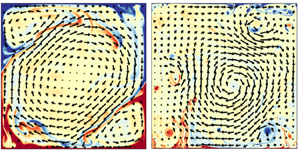
  $Ra$ (figure 4e–h), no stable LSC of domain size can be seen any more. Instead, one observes a main circulatory roll smaller than the domain and several satellite eddies orbit around it. Due to the squeezing from these satellite eddies, the main roll is unstable and wanders in the bulk region irregularly. Moreover, some thermal plumes can survive and travel through the strongly turbulent bulk region for a long time. As a result, the flow field becomes more fluctuating and disordered. These dramatic changes in flow patterns and dynamics can be seen clearly in the supplementary movies available at https://doi.org/10.1017/jfm.2024.847.

Figure 4. Instantaneous velocity–temperature fields for (a–d) the condensed state and (e–h) the uncondensed state for different  $Pr$: (a,e)
  $Pr=0.25$, (b,f)
  $Pr=0.7$, (c,g)
  $Pr=4.3$ and (d,h)
  $Pr=20$. The velocity is coded by the length and orientation of the vector, and the temperature is colour coded with red (blue) representing hot (cold) fluid. The
  $Ra$ number for each flow state is indicated on top of each subplot.
The change from a stable LSC to an unstable main roll can be characterized by the motions of their vortex centres. To do so, we first identify the largest roll from the instantaneous flow field. This is achieved by filtering the vorticity field  $\omega =\boldsymbol {\nabla } \times \boldsymbol{u}(\boldsymbol {x},t)$ with appropriate thresholds for different
  $Ra$ and
  $Pr$ numbers. The basic requirement to determine the threshold is that, after applying the threshold to the original vorticity field, the vortices with strong vorticities should be well distinguished and then extracted from the background flow. Taking the case with
  $Pr=4.3$ and
  $Ra=1 \times 10^{11}$ as an example, figure 5(a) shows that the flow is abundant of vortices with different sizes and strengths. By applying a threshold of
  $\omega <-8$ to the original vorticity field, the strong clockwise-rotating vortices, including the largest roll in the system, are identified (see figure 5b). These vortices were further sorted by their sizes and labelled with different colours. Then the centroid of the first labelled vortex is determined as the vortex centre of the largest roll, as indicated by a star in figure 5(c). As demonstrated in the supplementary movie, this method allows us to track the motion of the largest roll nicely.

Figure 5. Illustration of how to identify the vortex centre of the largest roll from the flow field. (a) A snapshot of the original vorticity field at  $Pr=4.3$ and
  $Ra=1 \times 10^{11}$. The vorticity is colour coded with blue (red) representing clockwise (anti-clockwise) rotating vortices. (b) The identified vortices after applying a filtered threshold of
  $\omega <-8$ to the vorticity field in (a). (c) The vortices in (b) are sorted by their sizes and labelled with different colours. The star indicates the identified vortex centre of the largest roll. Note that different thresholds (ranging from
  $\omega <-4$ to
  $\omega <-12$) have been tested for this case and they have little impact on the result.
The thus-determined trajectories of the vortex centre of the largest roll in different flow states are plotted in figure 6. It is seen that the vortex centre of the largest roll before the transition always stays near the domain's centre; in other words, its trajectory is ‘condensed’ in a limited area. By contrast, the vortex centre of the largest roll after the transition exhibits irregular motion and can explore the domain extensively; thus, its trajectory is ‘uncondensed’. Note that no appreciable sign of periodicity could be found by examining the autocorrelation functions of these trajectories, differing from the obvious periodically orbiting motion observed in a cylindrical cell of  $\varGamma = 2$ by Li et al. (Reference Li, Chen, Xu and Xi2022). Based on the distinct features of these trajectories, we term the flow states before and after the transition as the condensed and uncondensed states, respectively. It is worth noting that this terminology is the same as that in a previous study but from a different perspective (van der Poel et al. Reference van der Poel, Stevens, Sugiyama and Lohse2012). Here, we focus on the dynamics of the largest roll, while van der Poel et al. (Reference van der Poel, Stevens, Sugiyama and Lohse2012) adopted the notation of condensation in 2-D turbulence (Kraichnan Reference Kraichnan1967; Xia et al. Reference Xia, Byrne, Falkovich and Shats2011) in the sense that the energy is piled up to a scale of the domain size in the condensed state, whereas the largest roll in the uncondensed state is smaller than the system scale. However, as the energy cascade of RBC is always contaminated by the walls and other complicating factors (Xie & Huang Reference Xie and Huang2022), whether the present phenomenon could be understood by 2-D turbulence theory, which assumes homogeneity and isotropy of the flow, remains elusive and is outside the scope of this study.

Figure 6. The trajectories of the vortex centre of the largest roll in the condensed state (blue) and the uncondensed state (red) for different  $Pr$: (a)
  $Pr=0.25$, (b)
  $Pr=0.70$, (c)
  $Pr=4.3$ and (d)
  $Pr=20.0$. The
  $Ra$ number for each flow state is indicated in the subplots.
3.2. Determination of the transitional Rayleigh number  $Ra_{t}$

In addition to the change in the largest roll, another important feature of the flow state transition is the emergence of multiple satellite eddies with different sizes. This multi-scale feature could be captured by employing the Fourier mode analysis, which has been demonstrated as an efficient tool in previous studies of 2-D turbulent RBC (Chandra & Verma Reference Chandra and Verma2011; Wang et al. Reference Wang, Xia, Wang, Sun, Zhou and Wan2018; Xu et al. Reference Xu, Chen and Xi2021). Specifically, the instantaneous velocity fields are projected onto the Fourier basis as below:
 $$\begin{gather} u_x(x,z,t)=\sum_{m,n}\hat{u}_x(m,n,t)[2\sin(m{\rm \pi} x)\cos(n{\rm \pi} z)], \end{gather}$$
 $$\begin{gather}u_z(x,z,t)=\sum_{m,n}\hat{u}_z(m,n,t)[-2\cos(m{\rm \pi} x)\sin(n{\rm \pi} z)]. \end{gather}$$
Here,  $\hat {u}_i(m,n,t)$
  $(i=x,z)$ is the amplitude of the
  $(m,n)$ mode in the
  $i$ direction at time instant
  $t$, and the corresponding energy contained in the
  $(m,n)$ mode is
  $E^{m,n}(t)=|\hat {u}_x(m,n,t)|^2+|\hat {u}_z(m,n,t)|^2.$ Note that we have analysed the data by other methods such as proper orthogonal decomposition (Podvin & Sergent Reference Podvin and Sergent2015; Xu et al. Reference Xu, Chen and Xi2021). The results obtained are similar and the findings below are unaffected.
We first take the results obtained at  $Pr =4.3$ as an example for discussion. Figure 7(a,b) shows the time traces of the normalized energy contained in the first nine Fourier modes
  $E^{m,n}$ (i.e.
  $m$ and
  $n =1,2,3$) before and after the flow state transition. Here
  $E_{total}(t)$ represents the total energy of all Fourier modes at time instant
  $t$. It is seen that the system is dominated by the (1,1) and (2,2) modes before the transition, corresponding to the LSC and the corner rolls observed in the condensed state, respectively. Although the contributions from some other modes are also visible, their fluctuations in time are relatively gentle. When it goes to the uncondensed state, the (1,1) mode is still prevailing but becomes more fluctuating, consistent with the observation that the largest roll is unstable in this state. More importantly, vigorous fluctuations can be seen in the time traces of the normalized energy for almost all modes after the transition. This is in particular for the (1,2) and (2,1) modes, which are activated pronouncedly in the uncondensed state, in contrast to their negligible energies and fluctuations in the condensed case. As the (1,2) or (2,1) mode represents a flow structure with two horizontally or vertically stacked rolls, their activation could be attributed to the emergence of the satellite eddies that orbit around the main roll. It is their orbiting motions and interaction with the main roll that lead to the vigorous fluctuations observed here.

Figure 7. Time traces of the energy contained in the first nine Fourier modes  $E^{m,n}$ normalized by the total energy of all modes
  $E_{total}$ at
  $Pr = 4.3$: (a) an example in the condensed state and (b) an example in the uncondensed state. (c) The normalized r.m.s. values of
  $E^{m,n}$ as a function of
  $Ra$ at
  $Pr = 4.3$. The vertical dashed line indicates the location of the transitional
  $Ra$ number
  $Ra_t$. The grey symbols represent the cases with LSC reversals, which is consistent with the finding by Sugiyama et al. (Reference Sugiyama, Ni, Stevens, Chan, Zhou, Xi, Sun, Grossmann, Xia and Lohse2010).
To quantify how the energy fluctuations of different Fourier modes change during the transition, we plot their root-mean-square (r.m.s.) values  $E^{m,n}_{rms}$ as a function of
  $Ra$ in figure 7(c). Here,
  $E^{m,n}_{rms}$ is normalized by the time-averaged total energy of all Fourier modes
  $\langle E_{total}\rangle$. The grey symbols represent that LSC reversals can be observed for these cases, which makes the
  $Ra$ dependence of
  $E^{m,n}_{rms}/\langle E_{total}\rangle$ complicated. For
  $Ra>4\times 10^8$ without LSC reversals, the data first decreases with
  $Ra$ gradually and then jumps up abruptly at a transitional
  $Ra$ number
  $Ra_t$ for all modes. Visual inspection of the flow field confirms that it is in the vicinity of
  $Ra_t$ that the flow state transition occurs. Therefore, the abrupt change in
  $E^{m,n}_{rms}/\langle E_{total}\rangle$ can be used as an indicator of the transition. Since such a jump is most significant in the (1,2) and (2,1) modes, the value of
  $Ra_t$ can be determined by finding the location of the maximum growth rate of
  $E^{1,2}_{rms}$ or
  $E^{2,1}_{rms}$, which yields
  $Ra_t=7.7\times 10^9$ for
  $Pr=4.3$.
The above-discussed abrupt change in the energy fluctuations of Fourier modes can be found for all  $Pr$ explored in the present study. As shown in figure 8(a–h), although the detailed
  $Ra$-dependent trends of
  $E^{m,n}_{rms}/\langle E_{total}\rangle$ are different for different
  $Pr$, the (1,2) and (2,1) modes exhibit a similar sharp jump for all the cases. However, due to the unaffordable cost of running massive simulations near
  $Ra_t$ for all
  $Pr$, we did not determine the values of
  $Ra_t$ for other
  $Pr$ using the same method as that for
  $Pr=4.3$. Instead, we first locate the
  $Ra$ range where
  $E^{1,2}_{rms}$ (or
  $E^{2,1}_{rms}$) shows an abrupt increase, and then estimate
  $Ra_t$ as the average value of the two
  $Ra$ numbers just before and after this increase. The so-obtained
  $Ra_t$ is indicated by the dashed line in each subplot of figure 8(a–h), with its uncertainty represented by the shaded region. Quantitatively, one sees in figure 8(i) that
  $Ra_t$ increases with
  $Pr$ and can be fitted by a power law as
  $Ra_t=1.1\times 10^9 Pr^{1.41\pm 0.02}$. This scaling relation is also plotted in figure 1, which separates the two flow regimes, i.e. the condensed state and the uncondensed state in the phase diagram.

Figure 8. (a–h) The normalized r.m.s.values of the energy contained in the Fourier modes as a function of  $Ra$ for different
  $Pr$. Only the first four modes are shown for the clarity of presentation, as they are sufficient to reveal the transition behaviour. The vertical dashed line indicates the location of
  $Ra_t$ with the uncertainty marked by the shaded region. The grey symbols represent the cases with LSC reversals, which is consistent with the
  $Ra$-
$Ra$- $Pr$ phase diagram of LSC reversals reported by Sugiyama et al. (Reference Sugiyama, Ni, Stevens, Chan, Zhou, Xi, Sun, Grossmann, Xia and Lohse2010), further illustrating the reliability of our simulations. (i) Plot of
  $Ra_t$ as a function of
  $Pr$. The error bar represents the shaded region in (a–h). The dashed line is a power law fit to the data.
3.3. Bistability and the mechanism of the transition
To understand the scaling relation for  $Ra_t$, we now focus on the flow state in the vicinity of
  $Ra_t$ to see what happens during the transition. Again we take the cases at
  $Pr = 4.3$ as examples. By performing long-term simulations, it is found that the flow exhibits a bistability behaviour near
  $Ra_t$. This behaviour is characterized by spontaneous switching events between the condensed and uncondensed states, which can be quantified by the Nusselt number
  $Nu$ (dimensionless heat transport) and the Reynolds number
  $Re$ (dimensionless flow strength) as shown in figure 9(a,b). It is seen that both
  $Nu$ and
  $Re$ exhibit two plateaus with distinct time-averaged and r.m.s.values, and the switching events between the two plateaus in
  $Nu$ and
  $Re$ occur concurrently. Detailed inspection of the flow field indicates that the plateau with higher
  $Nu$ and smaller
  $Re$ corresponds to the condensed state (figure 9c), and that with lower
  $Nu$ and larger
  $Re$ corresponds to the uncondensed state (figure 9d). The larger r.m.s.values of
  $Nu$ and
  $Re$ for the uncondensed state are also clearly seen, in line with the vigorous energy fluctuations of the Fourier modes. It is worth noting that the lifetimes of the condensed and uncondensed states are comparable for the case shown in figure 9(a,b), both of which exceed 5000 free-fall times. As the
  $Ra$ number decreases (increases) slightly from
  $Ra=7.5\times 10^9$ to
  ${Ra=7.15\times 10^{9}}$ (
 ${Ra=7.85\times 10^{9}}$), it is found that the lifetime of the uncondensed (condensed) state decreases to about 1000 free-fall times and the flow becomes dominated by the condensed (uncondensed) state. This sensitive variation trend in lifetimes suggests that the uncondensed (condensed) state will disappear with
  $Ra$ further decreasing (increasing) away from
  $Ra_t$. In other words, the bistability behaviour exists in a limited
  $Ra$ number range near
  $Ra_t$, as highlighted by open triangles in figure 1. Similar responses of
  $Nu$ and
  $Re$ to multiple flow states and the corresponding lifetimes have been reported in previous studies of RBC under different configurations (Xi & Xia Reference Xi and Xia2008; Weiss & Ahlers Reference Weiss and Ahlers2011; van der Poel et al. Reference van der Poel, Stevens, Sugiyama and Lohse2012; Xie et al. Reference Xie, Ding and Xia2018; Zwirner et al. Reference Zwirner, Tilgner and Shishkina2020; Labarre et al. Reference Labarre, Fauve and Chibbaro2023), so we will not discuss this phenomenon further here. What we focus on is how the flow state transition occurs.

Figure 9. Time traces of (a)  $Nu$ and (b)
  $Re$ numbers for
  $Pr=4.3$ and
  $Ra=7.5\times 10^9$. The circles (diamonds) represent the short time-averaged values of
  $Nu$ (
 $Re$) over 50 free-fall times, corresponding to about five turnover times of the large-scale flow for this case. Four time intervals between successive switching events can be detected in panels (a,b). The time-averaged and r.m.s.values of
  $Nu$ (
 $Re$) during each time interval are represented by the red (blue) solid lines and the red (blue) shaded regions, respectively. The instantaneous flow fields at the moments marked by the two dashed lines are shown in panels (c,d), respectively. The velocity and temperature fields are coded in the same way as figure 4.
Through closely examining the bistability behaviour (see the supplementary movie), it is found that the switching event from the condensed state to the uncondensed case is triggered by some energetic plumes. These plumes, rather than dissipating most of their kinetic energy after travelling across the domain, intrude into the corner rolls when reaching the opposite boundary. As a result, the corner rolls become unstable and detach in the form of orbiting satellite eddies, which release extra thermal energy into the bulk flow and in turn result in more energetic plumes. This chain-reaction-like dynamics maintains the uncondensed state, explaining why the fluctuation is so violent in this state.
The above dynamical process reveals that the flow state transition occurs when the typical time for thermal plumes travelling across the domain  $\tau _{pt}\sim H/U$ becomes comparable to their typical dissipative time in the flow
  $\tau _{\epsilon _u} \sim U^2/\epsilon _u$. In other words, the two time scales are approximately balanced at the edge of the transition. By using the definition of the
  $Re$ number
  $Re=UH/\nu$ and the kinetic energy dissipation in the bulk region of the RBC
  $\epsilon _u=(\nu ^3/H^4)NuRaPr^{-2}$ (Lohse & Toschi Reference Lohse and Toschi2003), the balance of
  ${\tau _{pt} \sim \tau _{\epsilon _u}}$ suggests that the critical condition for the transition is given by
  ${Re^3 \sim Nu Ra Pr^{-2}}$. Note that the present time-scale balance analysis is a simple dimensional argument, so we have taken the maximum velocity in the flow and the globally averaged kinetic energy dissipation rate as the characteristic properties of thermal plumes, the latter of which is further connected to global responses of the system. This approximation is reasonable in the condensed state, as thermal plumes mostly follow the LSC's motion and primarily determine the global heat transport in this state (Xia et al. Reference Xia, Huang, Xie and Zhang2023). By substituting the corresponding scaling relations
  $Nu\sim Ra^{0.32}Pr^{-0.01}$ and
  $Re \sim Ra^{0.58}Pr^{-0.87}$ obtained in the condensed state (see figure 11 in the Appendix), we obtain that
  $Ra_t \sim Pr^{1.43}$, which agrees well with our numerical finding
  $Ra_t \sim Pr^{1.41}$. The same data analysis has been made in the uncondensed state. The global responses in this state are found to follow
  ${Nu \sim Ra^{0.27}Pr^{0.05}}$ and
  $Re \sim Ra^{0.61}Pr^{-0.94}$ (see figure 11 in the Appendix), leading to a slightly different transition scaling as
  $Ra_{t} \sim Pr^{1.55}$. Given the complex dynamics of the main roll and the satellite eddies in the uncondensed state, the discrepancy in the scaling exponents could be attributed to the dramatically different flow states and the uncertainty in estimating the characteristic properties of plumes.
The present phenomenological model can be further generalized to explain the effects of aspect ratio  $\varGamma$ on the transition. For domains with
  $\varGamma > 1$, because the plume travel distance remains to be the domain's height
  $H$, and the
  $Nu$ and
  $Re$ numbers depend weakly on
  $\varGamma$ (van der Poel et al. Reference van der Poel, Stevens, Sugiyama and Lohse2012; Wang et al. Reference Wang, Verzicco, Lohse and Shishkina2020), so the value of
  $Ra_t$ is expected to be insensitive to
  $\varGamma$. When
  $\varGamma < 1$, the flow pattern is featured by vertically stacked rolls (van der Poel et al. Reference van der Poel, Stevens, Sugiyama and Lohse2012). For this situation, the plume travel distance can be quantified as
  $\varGamma H$ without loss of generality, and then the critical condition for the transition turns out to follow
  $Re^3 \sim \varGamma Nu Ra Pr^{-2}$. By making use of the data at
  $Pr = 1$ in the range
  ${0.23 \leq \varGamma \leq 2/3}$ reported by van der Poel et al. (Reference van der Poel, Stevens, Sugiyama and Lohse2012), which can be described by
  $Nu\sim \varGamma ^{0.34}$ and
  $Re \sim \varGamma ^{0.79}$ roughly (see the Appendix), and assuming that the
  $Ra$ dependence of
  $Nu$ and
  $Re$ remains unchanged, we have
  $Ra_t \sim \varGamma ^{-2.46}$. These predictions on the
  $\varGamma$ dependence of
  $Ra_t$ are in good agreement with the findings by van der Poel et al. (Reference van der Poel, Stevens, Sugiyama and Lohse2012) mentioned in the introduction.
4. Summary and concluding remarks
In summary, we have carried out a systematic numerical study of 2-D turbulent RBC in a square domain over the Rayleigh number range  $10^7 \leq Ra \leq 2 \times 10^{11}$ and the Prandtl number range
  $0.25 \leq Pr \leq 20$, aiming to understand a previously noticed but less explored flow state transition. We first show in detail how the flow changes its morphology and dynamics substantially with increasing
  $Ra$: from the condensed state characterized by a stable LSC of domain size to the uncondensed state characterized by the emergence of orbiting satellite eddies and irregular wandering motion of the main roll. Then based on a sharp jump in the energy fluctuations of the Fourier modes during the transition, we obtain a scaling relation for the transitional
  $Ra$ number:
  $Ra_t=1.1\times 10^9Pr^{1.41}$. Finally, through a close examination of the bistability behaviour near
  $Ra_t$, we reveal that the critical condition for the transition is determined by the balance between the travel time of thermal plumes and their dissipation time in the flow, which is supported by our
  $Ra_t$-
 $Pr$ scaling relation. This physical picture also works for the transition observed in 2-D RBC with different aspect ratios (van der Poel et al. Reference van der Poel, Stevens, Sugiyama and Lohse2012).
To the best of our knowledge, the flow state transition observed in the present study has not been reported in the studies of both 3-D and quasi-2-D turbulent RBC so far. As discussed in 3.3, one important process during the transition is that the corner rolls become unstable due to the intrusion of some energetic plumes and then detach in the form of satellite eddies. This strong interaction between corner rolls and thermal plumes is enforced by the spatial confinement in 2-D geometry, which can also be achieved by using quasi-2-D configurations. Quasi-2-D RBC shares many similarities in the flow pattern and dynamics with its counterpart in two dimensions (Sugiyama et al. Reference Sugiyama, Ni, Stevens, Chan, Zhou, Xi, Sun, Grossmann, Xia and Lohse2010; He et al. Reference He, Fang, Gao, Huang and Bao2021; Li et al. Reference Li, He, Tian, Hao and Huang2021), suggesting that a similar flow state transition might occur in quasi-2-D RBC. However, the spatial confinement in quasi-2-D geometry increases the viscous drag on the flow and, thus, the energy dissipation (Chong & Xia Reference Chong and Xia2016; Huang & Xia Reference Huang and Xia2016; Xia et al. Reference Xia, Huang, Xie and Zhang2023), which would lead to a higher transitional  $Ra$ number according to the present study (similar to the situation of increasing the
  $Pr$ number). Therefore, to observe a similar flow state transition in quasi-2-D RBC, one should employ a strongly confined convection cell on one hand; but the spatial confinement should not be too severe on the other hand, so that the transitional
  $Ra$ number is not that high and can be reached by conventional experiments and numerical simulations. It is unknown a priori what degree of spatial confinement is appropriate. Some exploratory efforts are on the way and the findings, if any, will be reported in the future.
We end this paper by discussing more on the abrupt change in the energy fluctuations of the Fourier modes during the transition. This signal, together with the bistability behaviour observed in the vicinity of  $Ra_t$, implies that the flow state transition observed here is a phase transition. To confirm this, we adopt an order parameter based on the orientational correlation of the local velocity field to quantify the flow state, which was introduced in the studies of the so-called bacterial turbulence (Cisneros et al. Reference Cisneros, Kessler, Ganguly and Goldstein2011; Peng, Liu & Cheng Reference Peng, Liu and Cheng2021). To be specific, we first calculate the coherence of local velocities by
  $\phi _{i,local}=\langle \boldsymbol {n}_{i} \boldsymbol{\cdot } \boldsymbol {n}_{j} \rangle _{j=1,\ldots,4}$ as illustrated in figure 10(a). Here,
  $\boldsymbol {n}_{i} \boldsymbol {\cdot } \boldsymbol {n}_{j}$ stands for the cosine of the angle between adjacent velocity vectors and four neighbours are used for the average. Apparently,
  $\phi _{i,local} = 1$ represents a perfect-aligned local flow motion and decreasing
  $\phi _{i,local}$ indicates the velocity field becoming disordered. Thus, the spatiotemporal average
  $\phi =\langle \phi _{i,local} \rangle _{V,t}$ represents the global order of the flow. Note that the flow field has been downsampled to a resolution of
  $48\times 48$ vectors before calculating
  $\phi _{i,local}$, because neighbouring velocities are naturally aligned when the vector resolution is high. Different sampling densities (ranging from
  $16\times 16$ to
  $128\times 128$) have been tested and the results are little affected.

Figure 10. (a) Illustration of how to define the orientational correlation  $\phi _{i,local}$ from an instantaneous velocity field at
  $Pr=4.3$ and
  $Ra=1 \times 10^{11}$. (b) The order parameter
  $\phi =\langle \phi _{i,local} \rangle _{V,t}$ of the whole system as a function of
  $Ra$ at
  $Pr=4.3$. Here
  $\phi _u$ and
  $\phi _{u'}$ are obtained from the original and the fluctuating velocity fields, respectively. Panel (c) shows
  $\chi = |\partial \phi / \partial \log (Ra)|$ in the vicinity of the transition. The dashed lines represent data fittings based on the mean field approach:
  $\chi \propto [\log {Ra}-\log {Ra_{t}}]^{-1}$ with
  $Ra_{t}=7.7 \times 10^{9}$.
Figure 10(b) plots the  $Ra$ dependence of the thus-obtained order parameter
  $\phi$. It is seen that the data calculated from the fluctuating velocity field also shows a sharp jump near
  $Ra_t$, in line with the behaviour of the energy fluctuations of the Fourier modes. When the system is in the condensed state, the flow field is dominated by the (1,1) and (2,2) modes, whose temporal evolution are relatively gentle. Hence, the order parameter calculated from the fluctuating velocity field is comparatively small. When the flow gets into the uncondensed state, higher-order flow modes characterized by orbiting satellite eddies emerge. Their orbiting motions and interactions with the main roll result in significant temporal evolution in the velocity field. For this flow state, the fluctuating velocity field is dominated by those unsteady eddies (see figure 10a), which exhibit stronger spatial correlation and, thus, result in a larger order parameter. The stronger temporal evolution in the flow field also explains why the order parameter obtained from the original velocity field decreases, though slightly, during and after the transition, as the flow structures in the uncondensed state become less organized due to the interaction between multiple vortices. Despite the different variation trends of
  $\phi _u$ and
  $\phi _{u'}$, the absolute values of their gradients
  $\chi = |\partial \phi / \partial \log (Ra)|$ in the vicinity of transition could be well described by the mean field approach
  $\chi \propto [\log {Ra}-\log {Ra_{t}}]^{-1}$ (see figure 10c). This finding, reminiscent of the classical ferromagnetic phase transition (Pathria & Beale Reference Pathria and Beale2011), is striking to see in the present far-from-equilibrium system. A similar result was reported previously in an experimental study of turbulent von Kármán swirling flow (Cortet et al. Reference Cortet, Chiffaudel, Daviaud and Dubrulle2010), where the critical exponent for the transition is also
  $1$. In their study, the control parameter is the
  $Re$ number and the order parameter is defined by the space-averaged angular momentum, which are different from the present study but represent similar physical essences.
While it is unclear to us why the two vastly different flow configurations share the same critical exponent, we propose that the order parameter adopted here could be a unique indicator to quantify the transition behaviours observed in various turbulent flows (e.g. Seshasayanan, Benavides & Alexakis Reference Seshasayanan, Benavides and Alexakis2014; Benavides & Alexakis Reference Benavides and Alexakis2017; Seshasayanan & Alexakis Reference Seshasayanan and Alexakis2018; van Kan, Nemoto & Alexakis Reference van Kan, Nemoto and Alexakis2019; Musacchio & Boffetta Reference Musacchio and Boffetta2019; van Kan & Alexakis Reference van Kan and Alexakis2020; Linkmann, Hohmann & Eckhardt Reference Linkmann, Hohmann and Eckhardt2020; de Wit et al. Reference de Wit, Aguirre Guzmán, Clercx and Kunnen2022). Such abrupt transitions between different turbulent flow states have received great interest in recent years (see Alexakis & Biferale (Reference Alexakis and Biferale2018) for a review of this topic). It is interesting to see whether these diverse turbulent flows could fall into a universal class in terms of their critical exponents for the transition, which may help to understand the origin of this kind of non-equilibrium phase transition through a unifying framework.
Supplementary movies
Supplementary movies are available at https://doi.org/10.1017/jfm.2024.847.
Acknowledgements
We thank X. Zhu, J.-H. Xie, X.-G. Ma and K.L. Chong for their helpful discussions. S.-D.H. and Y.-C.X. are grateful to K.-Q. Xia for his guidance over the years and for his support of this study. The computational support from the Center for Computational Science and Engineering at Southern University of Science and Technology is also acknowledged.
Funding
This work is supported by the National Natural Science Foundation of China (grant nos. 11961160719, 92152104 and 11702128) and the Department of Science and Technology of Guangdong (no. 2023B1212060001). S.-D.H. acknowledges the support from the Pearl River Talent Recruitment Program (no. 2019QN01H691).
Declaration of interests
The authors report no conflict of interest.
Appendix. Simulation parameters; scaling relations of $Nu$ and $Re$ numbers


In this appendix, we detail the control parameters and numerical settings used for the present study in table 1. The global response parameters, i.e. the  $Nu$ and
  $Re$ numbers, are also provided in the table, and their
  $Ra$-
$Ra$- $Pr$ dependent scaling relations are plotted in figures 11(a)–11(d). Figures 11(e,f) show the data taken from van der Poel et al. (Reference van der Poel, Stevens, Sugiyama and Lohse2012). Note that their data at
  $\varGamma = 0.5$ exhibit some abnormal
  $Ra$-dependence in the range
  $10^7 < Ra < 10^{9}$, the reason of which is unclear to us, so only their data at
  $Ra = 10^{9}$ are considered here. The scaling relations obtained in figure 11 are used to estimate the transition scaling exponents for
  $Ra_t$ in § 3.3.
Table 1. The numerical details and the global response parameters of the present study. Here  $Pr$ and
  $Ra$ are the control parameters;
  $N_{x} \times N_{z}$ is the spatial resolution;
  $\varDelta _{g}$ is the maximal grid spacing;
  $\eta$ represents the Kolmogorov scale estimated by
  $\eta _{K}=HPr^{1/2}/[Ra(Nu-1)]^{1/4}$ when
  $Pr \leq 1$, or the Bachelor scale estimated by
  $\eta _{B}=\eta _{K}Pr^{-1/2}$ when
  $Pr > 1$;
  $N_{BL}$ is the number of grid points used for the boundary layer and
  $N_{BL}^{min}$ is the required minimum number according to Shishkina et al. (Reference Shishkina, Stevens, Grossmann and Lohse2010);
  $\tau _{f}$ is the time duration (in units of free-fall time) to get statistics;
  $Nu$,
$Nu$,  $Nu_{\epsilon _{\theta }}$ and
  $Nu_{\epsilon _{u}}$ are the dimensionless heat transfer efficiency obtained through the definition, the thermal and the kinetic dissipation rates, respectively;
  $\varLambda _{\theta }$ (
 $\varLambda _{u}$) is the relative error between
  $Nu$ and
  $Nu_{\epsilon _{\theta }}$ (
 $Nu_{\epsilon _{u}}$);
  $Re_{U_{rms}}$ and
  $Re_{U_{max}}$ are the Reynolds numbers characterized by different velocities
  $U$, where
  $U_{rms}=\sqrt { \langle u^{2}+w^{2} \rangle _{V,t}}$ and
  $U_{max}=\langle \max \{U\}\rangle _{t}$.


Figure 11. The compensated  $Nu$ and
  $Re$ as a function of
  $Ra$ for each
  $Pr$ obtained in the present study: panels (a,c) show the results in the condensed state and (b,d) are in the uncondensed state. Solid lines are the corresponding least-square fits, which yield
  $Nu \sim Ra^{0.32}Pr^{-0.01}$,
  $Re \sim Ra^{0.58}Pr^{-0.87}$ and
  $Nu \sim Ra^{0.27}Pr^{0.05}$,
  $Re \sim Ra^{0.61}Pr^{-0.94}$ for the condensed and uncondensed states, respectively. Since there exists no simple scaling law over a wide
  $Ra$ range (Grossmann & Lohse Reference Grossmann and Lohse2000), only the data one decade before or after
  $Ra_{t}$ are used to get the effective scaling exponents. Panels (e,f) show the
  $\varGamma$ dependencies of
  $Nu$ and
  $Re$, respectively. The data are taken from figure 2 of van der Poel et al. (Reference van der Poel, Stevens, Sugiyama and Lohse2012), and the least-square power law fitting yields
  $Nu\sim \varGamma ^{0.34}$ and
  $Re \sim \varGamma ^{0.79}$ roughly.


