The generalizability of an experiment is the extent to which it generates knowledge about causal relationships that is applicable beyond the narrow confines of the research site. How much further beyond is often a matter of great scientific importance. Vigorous discussion of the generalizability of findings occurs across all social scientific fields of inquiry (in economics: Levitt and List (Reference Levitt and List2007); psychology: Sears (Reference Sears1986); Henrich, Heine and Norenzayan (Reference Henrich, Heine and Norenzayan2010); education: Tipton (Reference Tipton2013); sociology: Lucas (Reference Lucas2003); and political science: McDermott (Reference McDermott2002)).
Concerns about the generalizability of findings usually fall into one of two categories: criticisms of the experimental context and criticisms of the experimental subjects. The first concern is a worry that an effect measured under experimental conditions is a poor guide to the effect in the “real world.” For example, a classic critique of survey experiments that investigate priming is that the effect, while “real” in the sense of being reliably reproducible in the survey context, is unimportant for the study of politics because primes have fleeting effects and political communication takes place in a competitive space where the marginal impact of a prime is likely to be canceled by a counterprime (Chong and Druckman Reference Chong and Druckman2010). Laboratory studies face a similar critique. Subjects may respond to the artificial context and obtrusive measurement in the lab in ways that do not generalize to the field.Footnote 1 Even well-designed field studies are sometimes accused of failing to generalize to the relevant political or policy decision because of some missing contextual feature.
A separate critique concerns the extent to which the study subjects are similar to the main population of interest. Because experimental subjects are very rarely drawn at random from any well-defined population, disagreements over whether treatment effect estimates obtained on a specific sample generalize to other places and times can be difficult to resolve. Within the social sciences, a point of some contention has been the increased use of online convenience samples, particularly samples obtained via Amazon’s Mechanical Turk (MTurk).Footnote 2 MTurk respondents often complete dozens of academic surveys over the course of a week, leading to concerns that such “professional” subjects are particularly savvy or susceptible to demand effects (Chandler et al. Reference Chandler, Paolacci, Peer, Mueller and Ratliff2015). These worries have been tempered somewhat by empirical studies that find that the MTurk population responds in ways similar to other populations (e.g., Berinsky, Huber and Lenz Reference Berinsky, Huber and Lenz2012), but concerns remain that subjects on MTurk differ from other subjects in both measured and unmeasured ways (Huff and Tingley Reference Huff and Tingley2015).
In the present study, I contribute to the growing literature on the replicability of survey experiments across platforms, following in the footsteps of two closely related studies. Mullinix et al. (Reference Mullinix, Leeper, Druckman and Freese2015) replicate 20 experiments and find a high degree of correspondence between estimates obtained on MTurk and on national probability samples, with a cross-sample correlation of 0.75.Footnote 3 Krupnikov and Levine (Reference Krupnikov and Levine2014) find that when treatments are expected to have different effects by subgroup, cross-sample correspondence is weaker. The correlation between their MTurk and YouGov estimates is 0.41.Footnote 4 To preview the results presented below, I find a strong degree of correspondence between national probability samples and MTurk: the cross-sample correlation of 40 pairs of average treatment effect estimates derived from 12 pairs of studies is 0.85 (df=38).
The remainder of this article will proceed as follows. First, I will present a theoretical framework that shows how the extent of treatment effect heterogeneity determines the generalizability of findings to other places and times. I will then present results from 15 replication studies, showing that in large part, original findings are replicated on both convenience and probability samples. I attribute this strong correspondence to the overall lack of treatment effect heterogeneity in these experiments; I conduct formal tests for unmodeled heterogeneity to bolster this claim.
TREATMENT EFFECT HETEROGENEITY AND GENERALIZABILITY
Findings from one site are generalizable to another site if the subjects, treatments, contexts, and outcome measures are the same—or would be the same—across both sites (Cronbach et al. Reference Cronbach and Shapiro1982; Coppock and Green Reference Coppock and Green2015). I define a site as the time, place, and group of units at and among which a causal process may hold. The most familiar kind of site is the research setting, with a well-defined group of subjects, a given research protocol, and implementation team. Typically, the purpose of an experiment conducted at a one site is to generalize knowledge to other sites where no experiment has been or will be conducted. For example, after an experiment conducted in one school district finds that a new curriculum is associated with large increases in student learning, we use that knowledge to infer both what would happen if the new curriculum were implemented in a different district, and what must have happened in the places where the curriculum was already in place.
The inferential target of a survey experiment conducted on a national probability sample of respondents is (often) the average treatment effect in the national population at a given moment in time, the population average treatment effect (PATE). The site of such an experiment might be an online survey administered to a random sample of adult Americans in 2012. The inferential target of the same experiment conducted on a convenience sample is a sample average treatment effect (SATE), where the sample in question is not drawn at random from the population. If a treatment engenders heterogeneous effects such that the distribution of treatment effects among those in the convenience sample is different from the distribution in the population, then the SATE will likely be different from the PATE.
When treatments, contexts, and outcome measures are held constant across sites, the generalizability of results obtained from one site to other sites depends only on the degree and nature of treatment effect heterogeneity. If treatments have constant effects (i.e., treatment effects are homogeneous), then the peculiarities of the experimental sample are irrelevant: what is learned from any subgroup can be generalized to any other population of interest. When treatments have heterogeneous effects, then the experimental sample might be very consequential. In order to assert that findings from one site are relevant for another site, a researcher must have direct or indirect knowledge of the distribution of treatment effects in both sites.
To illustrate the relationship between generalizability and heterogeneity, Figure 1 displays the potential outcomes and treatment effects for an entire population in two different scenarios. In the first scenario (represented in the left column of panels), treatment effects are heterogeneous, whereas in the second scenario, treatment effects are constant. The top row of panels displays the treated and untreated potential outcomes of the subjects and the bottom row displays the individual-level treatment effects (the difference between the treated and untreated potential outcomes).

Fig. 1 Implications of treatment effect heterogeneity for generalizability from convenience samples Note: SATE=sample average treatment effect; PATE=population average treatment effect.
An unobserved characteristic (U) of subjects is plotted on the horizontal axes of Figure 1. This characteristic represents something about subjects that is related to both their willingness to participate in survey experiments and their political attitudes. In both scenarios, U is negatively related to the untreated potential outcome (Y0): higher values of U are associated with lower values of Y0. This feature of the example represents how convenience samples may have different baseline political attitudes. Subjects on MTurk, for example, have been shown to hold more liberal attitudes than the public at large (Berinsky, Huber and Lenz Reference Berinsky, Huber and Lenz2012).
The untreated potential outcomes do not differ across scenarios, but the treated potential outcomes do. In scenario 1, effects are heterogeneous: higher values of U are associated with higher treatment effects, though the relationship depicted here is nonlinear. In scenario 2, treatment effects are homogeneous, so the unobserved characteristic U is independent of the differences in potential outcomes.
In both scenarios, imagine that two studies are conducted: one that samples from the entire population and a second that uses a convenience sample indicated by the shaded region. The population-level study targets the PATE, whereas the study conducted with the convenience sample targets a SATE. In scenario 1, the SATE and the PATE are different: generalizing from one research site to the other would lead to incorrect inferences. Note that this is a two-way street: with only an estimate of the PATE in hand, a researcher would make poor inferences about the SATE and vice versa. In scenario 2, the PATE and SATE are the same: generalizing from one site to another would be appropriate.
Figure 1 illustrates four points that are important to the study of generalizability. First, the fact that subjects may self-select into a study does not on its own mean that a study is not generalizable. Generalizability depends on whether treatment effect heterogeneity is independent of the (observed and unobserved) characteristics that determine self-selection. Second, even when baseline outcomes (Y0) are different in a self-selected sample from some population, the study may still be generalizable. The relevant theoretical question concerns the differences between potential outcomes (the treatment effects), not their levels. Third, when the characteristics that distinguish the population from that sample are unobserved, the PATE may not be informative about the SATE, that is, experiments that target the PATE should not be privileged over those that use convenience samples unless the PATE is truly the target of inference. Finally, it is important to distinguish systematic heterogeneity from idiosyncratic heterogeneity. When treatment effects vary systematically with measurable subject characteristics, then the generalizability problem reduces to measuring these characteristics, estimating conditional average treatment effects (CATEs), then reweighting these estimates by post-stratification. This reweighting can lead to estimates of either the SATE or the PATE, depending on the relevant target of inference. However, when treatment effects vary according to some unobserved characteristic of subjects (that also correlates with the probability of participation in a convenience sample), then no amount of post-stratification will license the generalization of convenience sample results to other sites.
RESULTS I: REPLICATIONS OF 12 SURVEY EXPERIMENTS
The approach adopted here is to replicate survey experiments originally conducted on nationally representative samples with MTurk subjects and, in three cases, with fresh nationally representative samples. The experiments selected for replication came in two batches. The first set of five (Haider-Markel and Joslyn Reference Haider-Markel and Joslyn2001; Peffley and Hurwitz Reference Peffley and Hurwitz2007; Transue Reference Transue2007; Chong and Druckman Reference Chong and Druckman2010; Nicholson Reference Nicholson2012) were selected for three reasons. First, as evidenced by their placement in top journals, these studies addressed some of the most pertinent political science questions. Second, these studies all had replication data available, either posted online, available on request, or completely described in summaries published in the original article. Finally, they were all conducted on probability samples drawn from some well-defined population. As shown in Table 1, the target population was not always the US national population. For example, in Haider-Markel and Joslyn (Reference Haider-Markel and Joslyn2001), the target of inference is the PATE among adult Kansans in 1999.
Table 1 Study Manifest
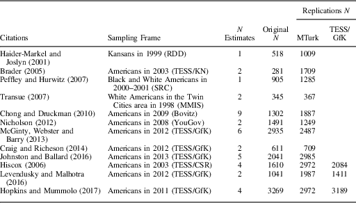
Note: MTurk=Mechanical Turk; TESS=Time-Sharing Experiments for the Social Sciences.
The second set of seven replications grew out of a collaboration with Time-Sharing Experiments for the Social Sciences (TESS), a National Science Foundation-supported organization that funds online survey experiments conducted on a national probability sample administered by GfK, a survey research firm. These studies are of high quality due in part to the peer review of study designs prior to data collection and to the TESS data-transparency procedures, by which raw data are posted one year after study completion. I selected seven studies, four of which (Brader Reference Brader2005; Nicholson Reference Nicholson2012; McGinty, Webster and Barry Reference McGinty, Webster and Barry2013; Craig and Richeson Reference Craig and Richeson2014) I replicated on MTurk, and three of which (Hiscox Reference Hiscox2006; Levendusky and Malhotra Reference Levendusky and Malhotra2016; Hopkins and Mummolo Reference Hopkins and Mummolo2017) I replicated both on MTurk and TESS/GfK. None of the seven I replicated were in the set of TESS studies replicated Mullinix et al. (Reference Mullinix, Leeper, Druckman and Freese2015). By and large, the replications were conducted with substantially larger samples than the original studies. All replications were conducted between January and September 2015. MTurk subjects were paid $1.00 for 5–10 minutes of their time and were eligible to participate if they were US residents and their previous work on the platform was accepted at least 95 percent of the time.
The studies cover a wide range of issue areas—gun control, immigration, the death penalty, the Patriot Act, home foreclosures, mental illness, free trade, health care, and polarization—and generally employ framing, priming, or information treatments designed to persuade subjects to change their political attitudes.Footnote 5 The particulars of each study’s treatments and outcome measures are detailed in the Online Appendix. With very few (minor) exceptions, the stimulus materials and outcome measures were identical across original and replication versions of the experiments.
The number of treatment effect estimates in each study (reported in Table 1) is a function of the number of treatment arms and dependent variables. In most cases, the studies employ multiple treatment arms and consider effects on a single dependent variable. In some cases, however, a single treatment versus control comparison is considered with respect to a range of dependent variables. I limited the number of dependent variables analyzed in each study to two. Where possible, I followed the original authors’ choices about which two dependent variables were most theoretically important; sometimes I had to use my best judgment to decide which were the two “main” outcome variables. I acknowledge that these choices introduce some subjectivity into the analysis. Mullinix et al. (Reference Mullinix, Leeper, Druckman and Freese2015) address this problem by focusing the analysis on the “first” dependent variable in each study, as determined by the temporal ordering of the dependent variables in the original TESS protocol. Their approach has the advantage of being automatically applicable across all studies but is no less subjective.
A wide range of analysis strategies were used in the original publications, including difference-in-means, difference-in-differences, ordinary least squares with covariate adjustment, subgroup analysis, and mediation analysis. To keep the analyses comparable, I reanalyzed all the original experiments using difference-in-means without conditioning on subgroups or adjusting for background characteristics.Footnote 6 Survey weights were incorporated where available. In all cases, I employed the Neyman variance estimator, equivalent to a standard variant of heteroskedasticity robust standard errors (Samii and Aronow Reference Samii and Aronow2012). I standardized all dependent variables by dividing by the control group standard deviation in the original study. I used the identical specifications across all versions of a study. The sample sizes reported in Table 1 refer to the number of subjects included in the analyses here. In some cases, this number is smaller than the sample size reported in the original articles because I have omitted some treatment arms (e.g., placebo treatments that do not figure in the main comparison of interest).
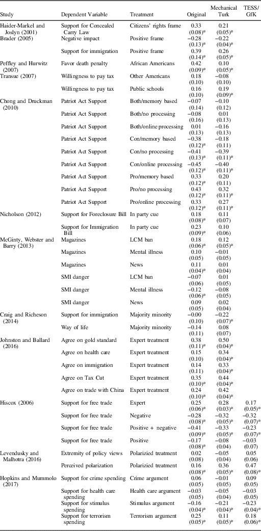
The study-by-study resultsFootnote 7 are presented in Figure 2. On the horizontal axis of each facet, I have plotted the average treatment effect estimates with 95 percent confidence intervals. The scale of the horizontal axis is different for each study, for easy inspection of the within-study correspondence across samples. On the vertical axes, I have plotted each treatment versus control comparison, by study version. The top nine facets compare two versions of each study (original and MTurk), while the bottom three compare three versions (original, MTurk, and TESS/GfK). The coefficients are ordered by the magnitude of the original study effects from most negative to most positive. This plot gives a first indication of the overall success of the replications: in no cases do the replications directly contradict one another, though there is some variation in the magnitudes of the estimated effects.
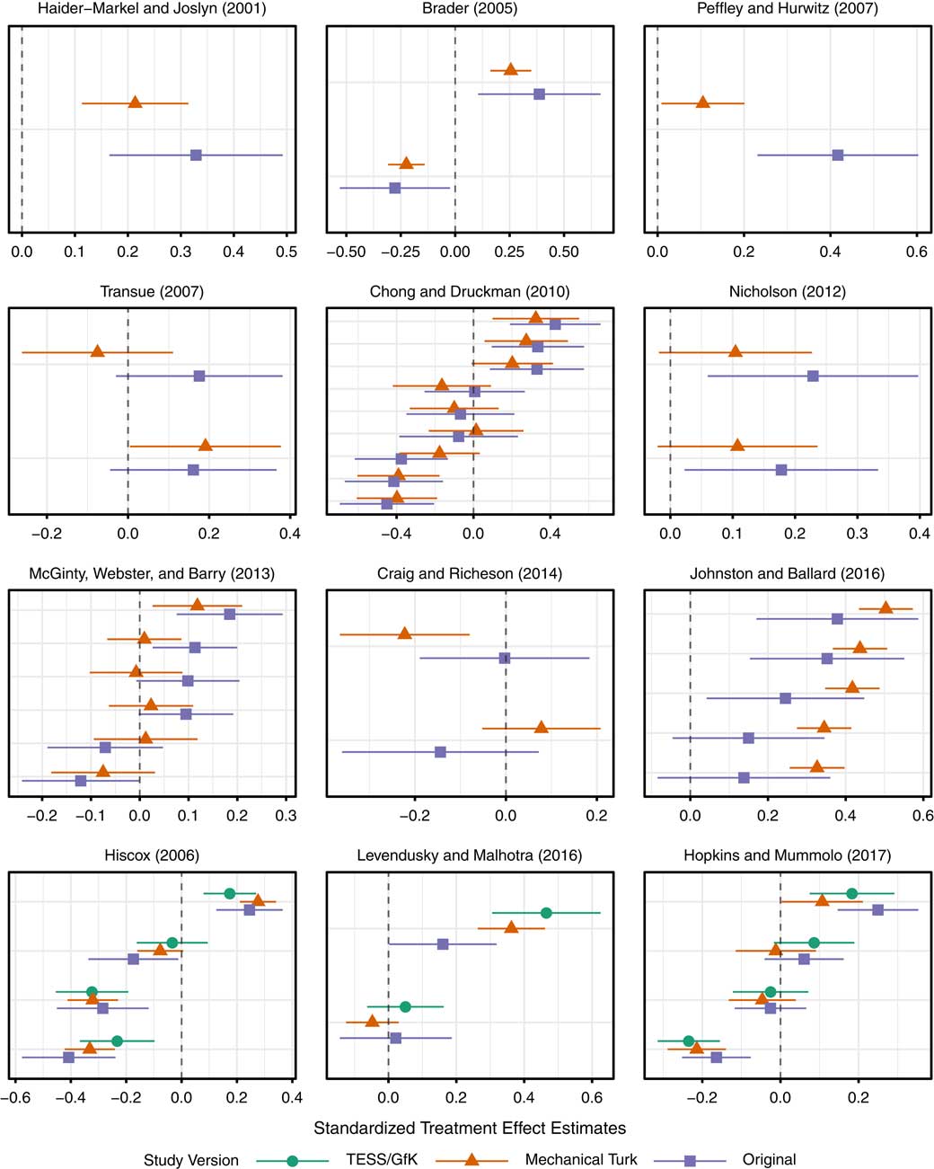
Fig. 2 Original and replication results of 12 studies Note: Each facet represents a study. Original treatment effect estimates are plotted with square points and replication treatment effect estimates are plotted with triangular (Mechanical Turk) or circular (Time-Sharing Experiments for the Social Sciences (TESS)/GfK) points.
Altogether, I estimated 40 original-MTurk pairs of coefficients. Of the 25 coefficients that were originally significant, 18 were significant in the MTurk replications, all with the correct sign. Of the 15 coefficients that were not originally significant, 11 were not significant in the MTurk replications either, for an overall replication rate (narrowly defined) of (18+11)/(25+15)=72.5 percent. In zero cases did two versions of the same study return statistically significant coefficients with opposite signs. The match rate of the sign and statistical significance of coefficients across studies is a crude measure of correspondence, as it conflates the power of the studies with their correspondence. For example, if all pairs of studies had a power of 0.01, that is, they only had a 1 percent chance of correctly rejecting a false null hypothesis of no average effect, then the match rate across pairs of studies would be close to 100 percent: nearly all coefficients would be deemed statistically insignificant. Measures of the replication rate that use the fraction of original studies within the 95 percent confidence interval of the replication (Open Science Collaboration 2015) or vice versa (Gilbert et al. Reference Gilbert, King, Pettigrew and Wilson2016) face a similar problem: lower powered studies appear to replicate at higher rates.
A better measure of the “replication rate” is the correlation of the standardized coefficients. Rather than relying on the artificial distinction between significant and nonsignificant, the correlation is a straightforward summary of the extent to which larger effects in the original studies are associated with larger effects in the replications. In the case of these 12 pairs of studies (40 coefficients), the correlation between the MTurk and original coefficients is 0.85 (df=38). This raw correlation is likely an underestimate of the true correlation in treatment effects because all pairs of treatment effect estimates are measured with noise. Figure 3 plots each coefficient with 95 percent confidence intervals for both the original and MTurk versions.
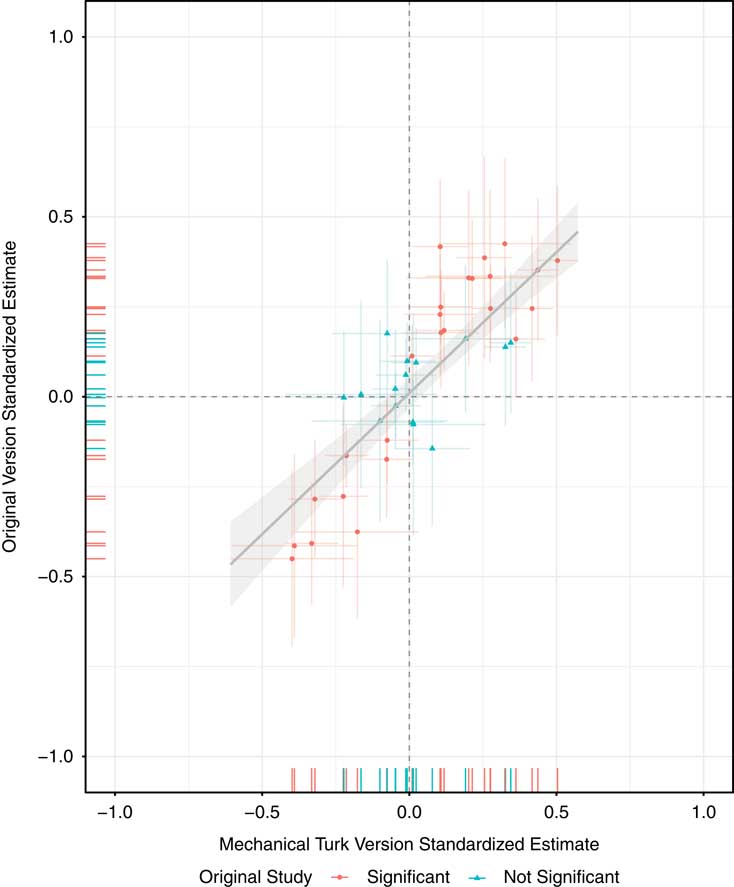
Fig. 3 Original coefficient estimates versus estimates obtained on Mechanical Turk Note: Each point represents a standardized treatment effect estimate in both the original study and the Mechanical Turk replication study.
For the three studies (ten coefficients) replicated in parallel on MTurk and on fresh TESS/GfK samples (Hiscox Reference Hiscox2006; Levendusky and Malhotra Reference Levendusky and Malhotra2016; Hopkins and Mummolo Reference Hopkins and Mummolo2017), the replication picture is even rosier. The correlation of the MTurk and original estimates is 0.90 (df=8); TESS/GfK estimates with the MTurk estimates, 0.96 (df=8); TESS/GfK with the original estimates, 0.85 (df=8).
All in all, these results show a strong pattern of replication across samples, lending credence to the idea that at least for the sorts of experiments studied here, estimates of causal effects obtained on MTurk samples tend to be similar to those obtained on probability samples.
RESULTS II: TESTING THE NULL OF TREATMENT EFFECT HOMOGENEITY
What can explain the strong degree of correspondence between the MTurk and nationally representative sample estimates of average causal effects? It could be that effects are heterogeneous within each sample—but this heterogeneity works out in such a way that the average effects across samples are approximately equal. This explanation is not out of the realm of possibility, and future work should consider whether the CATEs estimated within well-defined demographic subgroups (e.g., race, gender, and partisanship) also correspond across samples.
In this section, I report the results of empirical tests of a second theoretical explanation for the generalizabilty of these results across research sites: the treatments explored in this series of experiments have constant effects. If effects are homogeneous across subjects, then the differences in estimates obtained from different samples would be entirely due to sampling variability.
Building on advances in Fisher permutation tests, Ding, Feller and Miratrix (Reference Ding, Feller and Miratrix2016) propose a test of treatment effect heterogeneity that compares treated and control outcomes with a modified Kolmogorov–Smirnov (KS) statistic. The traditional KS statistic is the maximum observed difference between two cumulative distribution functions (CDFs), and is useful for summarizing the overall difference between two distributions. The modified KS statistic compares the CDFs of the de-meaned treated and control outcomes, thereby removing the estimated average treatment effect from the difference between the distributions and increasing the sensitivity of the test statistic to treatment effect heterogeneity.
The permutation test compares the observed values of the modified KS statistic to a simulated null distribution. This null distribution is constructed by imputing the missing potential outcomes for each subject under the null of constant effects, then simulating the distribution of the modified KS statistic under a large number of possible random assignments. One difficulty is choosing which constant effect to use for imputation. A natural choice is to use the estimated average treatment effect (ATE); however, as Ding, Feller and Miratrix (Reference Ding, Feller and Miratrix2016) show, this approach may lead to incorrect inferences. Instead, they advocate repeating the test for all plausible values of the constant ATE and reporting the maximum p-value. In practice, set of “all plausible” values of the is approximated by the 99.99 percent confidence interval around the estimated ATE.
This test, like other tests for treatment effect heterogeneity (Gerber and Green Reference Gerber and Green2012, 293–4), can be low-powered. To gauge the probability of correctly rejecting a false null hypothesis, I conducted a small simulation study that varied two parameters: the number of subjects per treatment arm and the degree of treatment effect heterogeneity. Equation 1 shows the potential outcomes function for subject i, where Z i is the treatment indicator and can take values of 0 or 1, σ τ the standard deviation of the treatment effects, and X i an idiosyncratic characteristic, drawn from a standard normal distribution. The larger σ τ , the larger the extent of treatment effect heterogeneity, and the more likely the test is to reject the null of constant effects. To put σ τ in perspective, consider a treatment with enormous effect heterogeneity: large positive effects of 0.5 standard units for half the sample, but large negative effects of 0.5 standard units for the other half. In this case the standard deviation of the treatment effects would be equal to 0.5. While the simple model of heterogeneity used for this simulation study does not necessarily reflect how the test would perform in other scenarios, it provides a first approximation of the sorts of heterogeneity typically envisioned by social scientists.
The results of the simulation study are presented in Figure 4. The MTurk versions of the experiments studied here typically employ 500 subjects per treatment arm, suggesting that we would be well powered (power≈0.8) to detect treatment effect heterogeneity on the scale of 0.2 SD, and moderately powered for 0.1 SD (power ≈0.6).
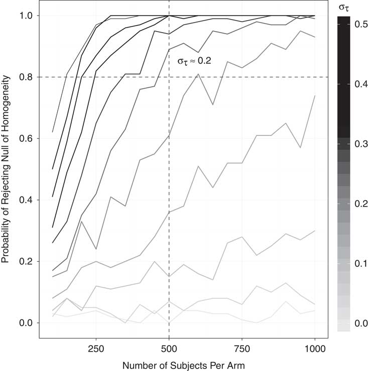
Fig. 4 Simulation study: power of the randomization test
The main results of the heterogeneity test applied to the present set of 27 studies (12 original and 15 replications) are displayed in Table 2. Among the original 12 studies, just 1 of the 40 treatment versus control comparisons revealed evidence of effect heterogeneity. Among the MTurk replications, 8 of 40 treatments were shown to have heterogeneous effects. On the TESS/GfK replications, 0 of 10 tests were significant. In only one case (Hiscox Reference Hiscox2006), did the same treatment versus control comparisons return a significant test statistic across samples. In order to guard against drawing false conclusions due to conducting many tests, I present the number of significant tests after correcting the p-values by the Holm (Reference Holm1979) correction in the last column of Table 2.Footnote 8
Table 2 Tests of Treatment Effect Heterogeneity

Note: TESS=Time-Sharing Experiments for the Social Sciences.
Far more often than not, we fail to reject the null of treatment effect homogeneity. Because we are relatively well powered to detect politically meaningful differences in treatment response, I conclude from this evidence that the treatment effect homogeneity explanation of the correspondence across experimental sites is plausible.
DISCUSSION
Levitt and List (Reference Levitt and List2007, p. 170) remind us that “Theory is the tool that permits us to take results from one environment to predict in another[.]” When the precise nature of treatments varies across sites, we need theory to distinguish the meaningful differences from the cosmetic ones. When the contexts differ across sites—public versus private interactions, field versus laboratory observations—theory is required to generalize from one to the other. When outcomes are measured differently, we rely on theory to predict how a causal process will express itself across sites.
In the results presented above, the treatments, contexts, and outcome measures were all held constant across sites by design. The only remaining impediment to the generalizability of the survey experimental findings from convenience samples to probability samples is the composition of the subject pools. If treatments have heterogeneous effects, researchers have to be careful not to generalize from a sample that has one distribution of treatment effects to populations that have different distributions of effects.
Before this replication exercise (and others like it such as Mullinix et al. Reference Mullinix, Leeper, Druckman and Freese2015; Krupnikov and Levine Reference Krupnikov and Levine2014), social scientists had a limited empirical basis on which to develop theories of treatment effect heterogeneity for the sorts of treatments explored here, which by and large attempt to persuade subjects of policy positions. Both within and across samples, the treatments studied here have exhibited muted treatment effect heterogeneity. Whatever differences (measured and unmeasured) there may be between the MTurk population and the population at large, they do not appear to interact with the treatments employed in these experiments in politically meaningful ways. In my view, it is this lack of heterogeneity that explains the overall correspondence across samples.
I echo the concerns of Mullinix et al. (Reference Mullinix, Leeper, Druckman and Freese2015), who caution that the pattern of strong probability/convenience sample correspondence does not imply that all survey experiments can be conducted with opt-in internet samples with no threats to inference more broadly. Indeed, the question is the extent of treatment effect heterogeneity. Some treatments of course have different effects for different subgroups and in such cases, an estimate obtained from a convenience sample may not generalize well. Future disagreements about whether a convenience sample can serve as a useful database from which to draw general inferences should be adjudicated on the basis of rival theories concerning treatment effect heterogeneity (or large, well-powered empirical demonstrations of such theories). Crucially, simply noting that convenience and probability samples differ in terms of their background characteristics is not sufficient for dismissing the results of experiments conducted on convenience samples.
Moreover, in an age of 9 percent response rates (Keeter et al. Reference Keeter, Hatley, Kennedy and Lau2017), even probability samples can only be considered representative of the population under the strong assumption that, after reweighting or post-stratification, no important differences remain between those who respond to the survey and the population. Probability samples may also only generalize to the moment in time they were conducted. Future research into the generalizability of treatment effects should also compare the extent to which probability samples drawn at one time correspond with probability samples drawn years later. Similar concerns may also extend to convenience samples, as some work suggests that the composition of the MTurk subject pool has changed in important ways over time (Stewart et al. Reference Stewart, Ungemach, Harris, Bartels, Newell, Paolacci and Chandler2015).
Finally, it is worth reflecting on the remarkable robustness of the experiments replicated here. Concerns over p-hacking (Simonsohn, Nelson and Simmons Reference Simonsohn, Nelson and Simmons2014), fishing (Humphreys, Sanchez de la Sierra and van der Windt Reference Humphreys, Sanchez de la Sierra and van der Windt2013), data snooping (White Reference White2000), and publication bias (Gerber et al. Reference Gerber, Malhotra, Dowling and Doherty2010; Franco, Malhotra and Simonovits Reference Franco, Malhotra and Simonovits2014) have lead many to express a great deal of skepticism over the reliability of results published in the scientific record (Ioannidis Reference Ioannidis2005). An effort to replicate 100 papers in psychology (Open Science Collaboration 2015) was largely viewed as a failure, with only one-third to one-half of papers replicating, depending on the measure. By contrast, the empirical results in this set of experiments were largely confirmed.
I speculate that this high replication rate may be explained in part by the procedure used to select studies for replication in the first place. I chose studies that had replication data available and whose treatment effect estimates were relatively precise. Further, the studies originally conducted on TESS underwent pre-implementation peer review, a process that might have either excluded theoretically tenuous studies or improved the design of chosen studies. Because these studies may have been of unusually high quality relative to the modal survey experiment in the social sciences, we should exercise caution when generalizing from this set of replications to all studies conducted on convenience samples.
Appendix
Table A1 Original and Replication Average Treatment Effect Estimates
