


1 Introduction
Several types of evidence, including the observed velocities of stars (Ghez et al.
Reference Ghez, Salim, Hornstein, Tanner, Lu, Morris, Becklin and Duchêne2005) and gas (Miyoshi et al.
Reference Miyoshi, Moran, Herrnstein, Greenhill, Nakai, Diamond and Inoue1995) near galactic centres and gravitational-wave signals indicative of black-hole (BH) mergers (Abbott et al.
Reference Abbott, Abbott, Abbott, Abernathy, Acernese, Ackley, Adams, Adams, Addesso and Adhikari2016), reveal BHs scattered throughout the visible universe with masses ranging from several to billions of solar masses. As a BH pulls in plasma from its surroundings, the plasma’s angular momentum causes the inflowing plasma to form a disk. If this accretion disk is geometrically thin but optically thick (‘a thin disk’), then turbulent viscosity converts a significant fraction of the plasma’s gravitational potential energy into thermal energy that is radiated away before the material reaches the central BH. In part because of this, thin disks are promising candidates for explaining much of the continuum emission from high-luminosity active galactic nuclei (AGN) and stellar-mass BHs in binary systems in their brighter states (Novikov & Thorne Reference Novikov, Thorne, Dewitt and Dewitt1973; Shakura & Sunyaev Reference Shakura and Sunyaev1973). Disks that are geometrically thick but optically thin (‘thick disks’) are generally much less luminous than thin disks, because plasma in the disk can fall into the BH before it radiates much of its thermal energy (Narayan & Yi Reference Narayan and Yi1994), become marginally unstable to convection, which suppresses mass inflow to the central BH (Quataert & Gruzinov Reference Quataert and Gruzinov2000), or become gravitationally unbound and flow outward (Blandford & Begelman Reference Blandford and Begelman1999). Thick disks are thought to be present around low-luminosity BHs, such as Sagittarius A
 $^{\ast }$
at the centre of our galaxy (Narayan & Yi Reference Narayan and Yi1994; Quataert & Gruzinov Reference Quataert and Gruzinov2000).
$^{\ast }$
at the centre of our galaxy (Narayan & Yi Reference Narayan and Yi1994; Quataert & Gruzinov Reference Quataert and Gruzinov2000).
BH/accretion-disk systems launch two types of outflows: non-collimated winds, which can be mildly relativistic or non-relativistic, and collimated, relativistic jets. The jets emanating from BH systems at the centres of galaxies are particularly striking, because they can span hundreds of kiloparsecs (Fanaroff & Riley Reference Fanaroff and Riley1974). Theoretical studies (e.g. Blandford & Znajek Reference Blandford and Znajek1977) and numerical simulations (De Villiers, Hawley & Krolik Reference De Villiers, Hawley and Krolik2003a ; McKinney & Gammie Reference McKinney and Gammie2004; Tchekhovskoy, Narayan & McKinney Reference Tchekhovskoy, Narayan and McKinney2011) have identified a promising mechanism for producing jets via a large-scale, ordered magnetic field that threads an accretion disk or the event horizon of a rotating BH. The rotation of the disk or BH coils up the magnetic-field lines, which then act as a spring, pushing material away from the disk along the spin axis.
Although this mechanism offers an explanation for jet formation and acceleration, it is not yet clear how the mass outflow rates and mechanical luminosities of jets and winds are determined. Nor is it clear what accelerates the particles that cause a jet, or the plasma at a jet’s base, to radiate. For example, it is unclear how to account for X-ray timing observations that indicate that many luminous AGN contain compact coronae – i.e. high-temperature, optically thin plasma – within a few gravitational radii of the central BH (Reis & Miller Reference Reis and Miller2013).
Clues to these puzzles may be offered by a system much closer to home. In one explanation for the heating and acceleration of the solar wind, convection-driven photospheric motions shake the footpoints of ‘open’ magnetic-field lines (i.e. field lines that connect directly to the interplanetary medium). This shaking launches Alfvén waves (AWs) that propagate along the magnetic-field lines, through coronal holes (open-field regions of the corona), and into the solar wind (Cranmer & van Ballegooijen Reference Cranmer and van Ballegooijen2005). Because the Alfvén speed varies with distance from the Sun, these outward-propagating AWs undergo partial non-WKB (Wentzel–Kramers–Brillouin) reflection (Heinemann & Olbert Reference Heinemann and Olbert1980; Velli Reference Velli1993). Counter-propagating AWs subsequently interact, which causes the AWs to become turbulent, which in turn causes AW energy to cascade from large wavelengths to small wavelengths and dissipate, heating the ambient plasma. This heating increases the plasma pressure, which, along with the wave pressure, accelerates the solar wind to supersonic speeds. This explanation for the solar wind’s origin is supported by numerous observational, theoretical and numerical studies (e.g. Cranmer & van Ballegooijen Reference Cranmer and van Ballegooijen2005; Cranmer, van Ballegooijen & Edgar Reference Cranmer, van Ballegooijen and Edgar2007; De Pontieu et al. Reference De Pontieu, McIntosh, Carlsson, Hansteen, Tarbell, Schrijver, Title, Shine, Tsuneta and Katsukawa2007; Verdini & Velli Reference Verdini and Velli2007; Hollweg, Cranmer & Chandran Reference Hollweg, Cranmer and Chandran2010; Verdini et al. Reference Verdini, Velli, Matthaeus, Oughton and Dmitruk2010; Chandran et al. Reference Chandran, Dennis, Quataert and Bale2011; Perez & Chandran Reference Perez and Chandran2013; van der Holst et al. Reference van der Holst, Sokolov, Meng, Jin, Manchester IV, Tóth and Gombosi2014; Usmanov, Goldstein & Matthaeus Reference Usmanov, Goldstein and Matthaeus2014; van Ballegooijen & Asgari-Targhi Reference van Ballegooijen and Asgari-Targhi2016, Reference van Ballegooijen and Asgari-Targhi2017). Turbulence plays a key role in this model, because the large-wavelength AWs launched by the Sun are damped so weakly that, without turbulence, they would reach the distant interplanetary medium without appreciably damping or heating the plasma (Barnes Reference Barnes1966). Wave reflection is a critical component of the model because the Sun launches only outward-propagating waves, and AWs interact to produce turbulence only when there is a mix of counter-propagating AWs in the plasma rest frame (Iroshnikov Reference Iroshnikov1963; Kraichnan Reference Kraichnan1965).
In this paper, we explore the possibility that similar physical processes contribute to the generation of accretion-disk coronae and jets. In particular, we consider the fate of AWs that are launched by a turbulent accretion disk into the disk’s corona and an overlying outflow. To allow for space–time curvature, relativistic fluid velocities, relativistic Alfvén speeds and relativistic thermal velocities, we work within the framework of general relativistic magnetohydrodynamics (GRMHD). Previous studies have investigated the heating of accretion-disk coronae by the reconnection of magnetic loop structures (e.g. Galeev, Rosner & Vaiana Reference Galeev, Rosner and Vaiana1979; Uzdensky & Goodman Reference Uzdensky and Goodman2008). Our work focuses on AW turbulence rather than magnetic reconnection, and open-field regions rather than closed magnetic loops.
The remainder of this paper is organized as follows. In § 2 we derive a set of equations that describes AW propagation, reflection and nonlinear interactions in an inhomogeneous background flow. In § 3 we specialize to the case of a time-independent and axisymmetric background and solve analytically for the mean-square AW amplitude and turbulent heating rate as functions of position. In § 4 we apply our results to the corona and outflow overlying a thin accretion disk in the
 $\unicode[STIX]{x1D6FC}$
-disk model (Novikov & Thorne Reference Novikov, Thorne, Dewitt and Dewitt1973; Shakura & Sunyaev Reference Shakura and Sunyaev1973). In § 5 we derive a set of averaged GRMHD equations in which AW turbulence is treated using a sub-grid model. These equations complement the results of § 2 by describing how AW turbulence influences the background flow via turbulent heating and momentum deposition.
$\unicode[STIX]{x1D6FC}$
-disk model (Novikov & Thorne Reference Novikov, Thorne, Dewitt and Dewitt1973; Shakura & Sunyaev Reference Shakura and Sunyaev1973). In § 5 we derive a set of averaged GRMHD equations in which AW turbulence is treated using a sub-grid model. These equations complement the results of § 2 by describing how AW turbulence influences the background flow via turbulent heating and momentum deposition.
2 Reflection-driven Alfvén-wave turbulence in general relativity
GRMHD describes a highly conducting magnetized fluid under the assumption that the Lorentz force vanishes for a charged particle at rest in the local plasma frame. This assumption simplifies the source-free subset of Maxwell’s equations and the electromagnetic contribution to the stress–energy tensor (see, e.g. Anile Reference Anile1989; Gammie, McKinney & Tóth Reference Gammie, McKinney and Tóth2003). A GRMHD fluid is described by the equation of mass conservation,
 $$\begin{eqnarray}(\unicode[STIX]{x1D70C}u^{\unicode[STIX]{x1D708}})_{;\unicode[STIX]{x1D708}}=0,\end{eqnarray}$$
the stress–energy equation,
 $$\begin{eqnarray}{T^{\unicode[STIX]{x1D707}\unicode[STIX]{x1D708}}}_{;\unicode[STIX]{x1D708}}=0,\end{eqnarray}$$
and the relativistic induction equation,
 $$\begin{eqnarray}(b^{\unicode[STIX]{x1D707}}u^{\unicode[STIX]{x1D708}}-b^{\unicode[STIX]{x1D708}}u^{\unicode[STIX]{x1D707}})_{;\unicode[STIX]{x1D708}}=0,\end{eqnarray}$$
where
 $\unicode[STIX]{x1D70C}$
is the mass density,
$\unicode[STIX]{x1D70C}$
is the mass density,
 $u^{\unicode[STIX]{x1D707}}$
is the 4-velocity,
$u^{\unicode[STIX]{x1D707}}$
is the 4-velocity,
 $$\begin{eqnarray}T^{\unicode[STIX]{x1D707}\unicode[STIX]{x1D708}}={\mathcal{E}}u^{\unicode[STIX]{x1D707}}u^{\unicode[STIX]{x1D708}}+\left(p+\frac{b^{2}}{2}\right)g^{\unicode[STIX]{x1D707}\unicode[STIX]{x1D708}}-b^{\unicode[STIX]{x1D707}}b^{\unicode[STIX]{x1D708}}\end{eqnarray}$$
is the GRMHD stress–energy tensor,
 $$\begin{eqnarray}b^{\unicode[STIX]{x1D707}}=\frac{1}{2}\unicode[STIX]{x1D716}^{\unicode[STIX]{x1D707}\unicode[STIX]{x1D708}\unicode[STIX]{x1D705}\unicode[STIX]{x03BB}}u_{\unicode[STIX]{x1D708}}F_{\unicode[STIX]{x03BB}\unicode[STIX]{x1D705}}\end{eqnarray}$$
is the magnetic-field 4-vector,
 $b^{2}=b^{\unicode[STIX]{x1D707}}b_{\unicode[STIX]{x1D707}}$
,
$b^{2}=b^{\unicode[STIX]{x1D707}}b_{\unicode[STIX]{x1D707}}$
,
 $F_{\unicode[STIX]{x03BB}\unicode[STIX]{x1D705}}$
is the Faraday tensor divided by
$F_{\unicode[STIX]{x03BB}\unicode[STIX]{x1D705}}$
is the Faraday tensor divided by
 $\sqrt{4\unicode[STIX]{x03C0}}$
,
$\sqrt{4\unicode[STIX]{x03C0}}$
,
 $\unicode[STIX]{x1D716}^{\unicode[STIX]{x1D707}\unicode[STIX]{x1D708}\unicode[STIX]{x1D705}\unicode[STIX]{x03BB}}$
is the Levi-Civita tensor,
$\unicode[STIX]{x1D716}^{\unicode[STIX]{x1D707}\unicode[STIX]{x1D708}\unicode[STIX]{x1D705}\unicode[STIX]{x03BB}}$
is the Levi-Civita tensor,
 $$\begin{eqnarray}{\mathcal{E}}=\unicode[STIX]{x1D70C}+u+p+b^{2},\end{eqnarray}$$
 $u$
(without indices) is the internal energy,
$u$
(without indices) is the internal energy,
 $p$
is the pressure,
$p$
is the pressure,
 $g_{\unicode[STIX]{x1D707}\unicode[STIX]{x1D708}}$
is the metric tensor and the units have been chosen so that the speed of light is 1 (Komissarov Reference Komissarov1999; Gammie et al.
Reference Gammie, McKinney and Tóth2003). The semicolon subscripts indicate covariant differentiation, repeated indices are summed and Greek indices range from 0 to 3. The 4-velocity satisfies
$g_{\unicode[STIX]{x1D707}\unicode[STIX]{x1D708}}$
is the metric tensor and the units have been chosen so that the speed of light is 1 (Komissarov Reference Komissarov1999; Gammie et al.
Reference Gammie, McKinney and Tóth2003). The semicolon subscripts indicate covariant differentiation, repeated indices are summed and Greek indices range from 0 to 3. The 4-velocity satisfies
 $$\begin{eqnarray}u^{\unicode[STIX]{x1D707}}u_{\unicode[STIX]{x1D707}}=-1,\end{eqnarray}$$
and it follows from (2.5) that
 $$\begin{eqnarray}u_{\unicode[STIX]{x1D707}}b^{\unicode[STIX]{x1D707}}=0.\end{eqnarray}$$
The magnetic-field 3-vector is given by
 $$\begin{eqnarray}B^{i}=b^{i}u^{t}-b^{t}u^{i},\end{eqnarray}$$
where Latin indices range from 1 to 3, and
 $t$
indices indicate the time component. Equation (2.9) can be inverted using (2.7) and (2.8) to give (Gammie et al.
Reference Gammie, McKinney and Tóth2003)
$t$
indices indicate the time component. Equation (2.9) can be inverted using (2.7) and (2.8) to give (Gammie et al.
Reference Gammie, McKinney and Tóth2003)
 $$\begin{eqnarray}b^{t}=B^{i}u^{\unicode[STIX]{x1D707}}g_{i\unicode[STIX]{x1D707}}\qquad b^{i}=\frac{B^{i}+b^{t}u^{i}}{u^{t}}.\end{eqnarray}$$
Equation (2.3) can then be rewritten as the two equations
 $$\begin{eqnarray}\frac{1}{\sqrt{-g}}\unicode[STIX]{x2202}_{i}\left(\sqrt{-g}B^{i}\right)=0\end{eqnarray}$$
and
 $$\begin{eqnarray}\unicode[STIX]{x2202}_{t}\left(\sqrt{-g}B^{i}\right)=\unicode[STIX]{x2202}_{j}\left[\sqrt{-g}(B^{\,j}v^{i}-B^{i}v^{\,j})\right],\end{eqnarray}$$
where
 $\unicode[STIX]{x2202}_{\unicode[STIX]{x1D707}}$
indicates differentiation with respect to coordinate
$\unicode[STIX]{x2202}_{\unicode[STIX]{x1D707}}$
indicates differentiation with respect to coordinate
 $\unicode[STIX]{x1D707}$
,
$\unicode[STIX]{x1D707}$
,
 $g$
is the determinant of the metric tensor and
$g$
is the determinant of the metric tensor and
 $v^{i}=u^{i}/u^{t}$
is the fluid 3-velocity (Gammie et al.
Reference Gammie, McKinney and Tóth2003). As described in § 5,
$v^{i}=u^{i}/u^{t}$
is the fluid 3-velocity (Gammie et al.
Reference Gammie, McKinney and Tóth2003). As described in § 5,
 $b^{\unicode[STIX]{x1D707}}$
is the magnetic field in the fluid frame (in the sense that is explained prior to (5.4)), while
$b^{\unicode[STIX]{x1D707}}$
is the magnetic field in the fluid frame (in the sense that is explained prior to (5.4)), while
 $B^{i}$
is the ‘laboratory-frame’ magnetic field when
$B^{i}$
is the ‘laboratory-frame’ magnetic field when
 $g^{tt}=-1$
.
$g^{tt}=-1$
.
2.1 An Elsasser-like formulation of GRMHD
Elsasser (Reference Elsasser1950) reformulated non-relativistic MHD, obtaining a set of equations that is useful for studying AWs and AW turbulence. We obtain an Elasser-like formulation of GRMHD by multiplying (2.3) by
 $\pm {\mathcal{E}}^{1/2}$
, adding the resulting expression to (2.2) and then dividing by
$\pm {\mathcal{E}}^{1/2}$
, adding the resulting expression to (2.2) and then dividing by
 ${\mathcal{E}}$
. This yields
${\mathcal{E}}$
. This yields
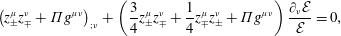 $$\begin{eqnarray}\left(z_{\pm }^{\unicode[STIX]{x1D707}}z_{\mp }^{\unicode[STIX]{x1D708}}+\unicode[STIX]{x1D6F1}g^{\unicode[STIX]{x1D707}\unicode[STIX]{x1D708}}\right)_{;\unicode[STIX]{x1D708}}+\left(\frac{3}{4}z_{\pm }^{\unicode[STIX]{x1D707}}z_{\mp }^{\unicode[STIX]{x1D708}}+\frac{1}{4}z_{\mp }^{\unicode[STIX]{x1D707}}z_{\pm }^{\unicode[STIX]{x1D708}}+\unicode[STIX]{x1D6F1}g^{\unicode[STIX]{x1D707}\unicode[STIX]{x1D708}}\right)\frac{\unicode[STIX]{x2202}_{\unicode[STIX]{x1D708}}{\mathcal{E}}}{{\mathcal{E}}}=0,\end{eqnarray}$$
where
 $$\begin{eqnarray}z_{\pm }^{\unicode[STIX]{x1D707}}=u^{\unicode[STIX]{x1D707}}\mp \frac{b^{\unicode[STIX]{x1D707}}}{{\mathcal{E}}^{1/2}}\qquad \unicode[STIX]{x1D6F1}=\frac{2p+b^{2}}{2{\mathcal{E}}}.\end{eqnarray}$$
2.2 Background quantities, fluctuations and the average fluid rest frame
We assume that each property of the fluid is the sum of a smoothly varying background value plus a fluctuation,
 $$\begin{eqnarray}u^{\unicode[STIX]{x1D707}}=\overline{u^{\unicode[STIX]{x1D707}}}+\unicode[STIX]{x1D6FF}u^{\unicode[STIX]{x1D707}}\qquad b^{\unicode[STIX]{x1D707}}=\overline{b^{\unicode[STIX]{x1D707}}}+\unicode[STIX]{x1D6FF}b^{\unicode[STIX]{x1D707}}\qquad \text{etc.}\end{eqnarray}$$
We construct an ‘average fluid rest frame’ (AFRF) at each point by first transforming to locally Galilean coordinates and then carrying out a Lorentz transformation that causes
 $\overline{u^{i}}$
to vanish while leaving the metric in Minkowski form at that point. We define
$\overline{u^{i}}$
to vanish while leaving the metric in Minkowski form at that point. We define
 $\unicode[STIX]{x03BB}$
to be the perpendicular correlation length (i.e. the correlation length measured perpendicular to
$\unicode[STIX]{x03BB}$
to be the perpendicular correlation length (i.e. the correlation length measured perpendicular to
 $\overline{B^{i}}$
) of the velocity and magnetic-field fluctuations in the AFRF, and
$\overline{B^{i}}$
) of the velocity and magnetic-field fluctuations in the AFRF, and
 $L$
to be the characteristic length scale of the background quantities and
$L$
to be the characteristic length scale of the background quantities and
 $g_{\unicode[STIX]{x1D707}\unicode[STIX]{x1D708}}$
in the AFRF. We assume that
$g_{\unicode[STIX]{x1D707}\unicode[STIX]{x1D708}}$
in the AFRF. We assume that
 $$\begin{eqnarray}\unicode[STIX]{x03BB}/L\sim O(\unicode[STIX]{x1D716}),\end{eqnarray}$$
where
 $\unicode[STIX]{x1D716}$
(without indices) is a small parameter. We use the notation
$\unicode[STIX]{x1D716}$
(without indices) is a small parameter. We use the notation
 $\langle \ldots \rangle$
to denote a volume average within a sphere of radius
$\langle \ldots \rangle$
to denote a volume average within a sphere of radius
 $d$
in the AFRF, with
$d$
in the AFRF, with
 $\unicode[STIX]{x03BB}\ll d\ll L$
. For any vector
$\unicode[STIX]{x03BB}\ll d\ll L$
. For any vector
 $f^{\unicode[STIX]{x1D707}}$
, we assume that the following assertions lead to negligible error:
$f^{\unicode[STIX]{x1D707}}$
, we assume that the following assertions lead to negligible error:
 $\langle \,f^{\unicode[STIX]{x1D707}}\rangle$
is a vector,
$\langle \,f^{\unicode[STIX]{x1D707}}\rangle$
is a vector,
 $\langle \langle \,f^{\unicode[STIX]{x1D707}}\rangle \rangle =\langle \,f^{\unicode[STIX]{x1D707}}\rangle =\overline{f^{\unicode[STIX]{x1D707}}}$
and
$\langle \langle \,f^{\unicode[STIX]{x1D707}}\rangle \rangle =\langle \,f^{\unicode[STIX]{x1D707}}\rangle =\overline{f^{\unicode[STIX]{x1D707}}}$
and
 $\langle \,{f^{\unicode[STIX]{x1D707}}}_{;\unicode[STIX]{x1D708}}\rangle =\langle \,f^{\unicode[STIX]{x1D707}}\rangle _{;\unicode[STIX]{x1D708}}$
, with analogous statements for scalars and tensors. We note that
$\langle \,{f^{\unicode[STIX]{x1D707}}}_{;\unicode[STIX]{x1D708}}\rangle =\langle \,f^{\unicode[STIX]{x1D707}}\rangle _{;\unicode[STIX]{x1D708}}$
, with analogous statements for scalars and tensors. We note that
 $\overline{u^{\unicode[STIX]{x1D707}}}$
is not a unit vector in the sense of (2.7) and is therefore not a 4-velocity. It is merely the local spatial average, in the AFRF, of
$\overline{u^{\unicode[STIX]{x1D707}}}$
is not a unit vector in the sense of (2.7) and is therefore not a 4-velocity. It is merely the local spatial average, in the AFRF, of
 $u^{\unicode[STIX]{x1D707}}$
. The 4-velocity of the AFRF is given in (5.1) below.
$u^{\unicode[STIX]{x1D707}}$
. The 4-velocity of the AFRF is given in (5.1) below.
2.3 General relativistic reduced MHD in an inhomogeneous background
To motivate the next step in our analysis, we return for a moment to the solar analogy. Spacecraft measurements indicate that
 $B^{i}$
and
$B^{i}$
and
 $v^{i}$
fluctuations in the solar wind are mostly transverse (orthogonal to
$v^{i}$
fluctuations in the solar wind are mostly transverse (orthogonal to
 $\overline{B^{i}}$
) and non-compressive (Klein, Roberts & Goldstein Reference Klein, Roberts and Goldstein1991; Horbury et al.
Reference Horbury, Balogh, Forsyth and Smith1995; Tu & Marsch Reference Tu and Marsch1995). One reason for this is that the dominant dissipation mechanism for slow magnetosonic modes and entropy modes, turbulent mixing, causes the energy of these compressive modes to decay on the time scale
$\overline{B^{i}}$
) and non-compressive (Klein, Roberts & Goldstein Reference Klein, Roberts and Goldstein1991; Horbury et al.
Reference Horbury, Balogh, Forsyth and Smith1995; Tu & Marsch Reference Tu and Marsch1995). One reason for this is that the dominant dissipation mechanism for slow magnetosonic modes and entropy modes, turbulent mixing, causes the energy of these compressive modes to decay on the time scale
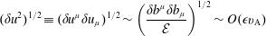
 $\unicode[STIX]{x03BB}/\unicode[STIX]{x1D6FF}u_{\text{rms}}$
, where
$\unicode[STIX]{x03BB}/\unicode[STIX]{x1D6FF}u_{\text{rms}}$
, where
 $\unicode[STIX]{x1D6FF}u_{\text{rms}}$
is the root-mean-square (r.m.s.) amplitude of the velocity fluctuations (Schekochihin et al.
Reference Schekochihin, Parker, Highcock, Dellar, Dorland and Hammett2016). This time scale is shorter than the energy-decay time scale for outward-propagating, non-compressive, AW fluctuations, which is
$\unicode[STIX]{x1D6FF}u_{\text{rms}}$
is the root-mean-square (r.m.s.) amplitude of the velocity fluctuations (Schekochihin et al.
Reference Schekochihin, Parker, Highcock, Dellar, Dorland and Hammett2016). This time scale is shorter than the energy-decay time scale for outward-propagating, non-compressive, AW fluctuations, which is
 ${\sim}\unicode[STIX]{x03BB}/\unicode[STIX]{x1D6FF}u_{\text{inward}}$
(Iroshnikov Reference Iroshnikov1963; Kraichnan Reference Kraichnan1965), where
${\sim}\unicode[STIX]{x03BB}/\unicode[STIX]{x1D6FF}u_{\text{inward}}$
(Iroshnikov Reference Iroshnikov1963; Kraichnan Reference Kraichnan1965), where
 $\unicode[STIX]{x1D6FF}u_{\text{inward}}$
is the r.m.s. velocity fluctuation of the inward-propagating AWs. The inequality
$\unicode[STIX]{x1D6FF}u_{\text{inward}}$
is the r.m.s. velocity fluctuation of the inward-propagating AWs. The inequality
 $\unicode[STIX]{x03BB}/\unicode[STIX]{x1D6FF}u_{\text{rms}}\ll \unicode[STIX]{x03BB}/\unicode[STIX]{x1D6FF}u_{\text{inward}}$
follows from in situ measurements (Bavassano, Pietropaolo & Bruno Reference Bavassano, Pietropaolo and Bruno2000) and numerical models (Cranmer & van Ballegooijen Reference Cranmer and van Ballegooijen2005; Verdini & Velli Reference Verdini and Velli2007; Perez & Chandran Reference Perez and Chandran2013; van Ballegooijen & Asgari-Targhi Reference van Ballegooijen and Asgari-Targhi2016) that show that outward-propagating AWs have much larger amplitudes than inward-propagating AWs in the near-Sun solar wind. The other compressive MHD mode, the fast magnetosonic mode, has an even smaller amplitude in the solar wind than the slow magnetosonic mode (Yao et al.
Reference Yao, He, Marsch, Tu, Pedersen, Rème and Trotignon2011; Howes et al.
Reference Howes, Bale, Klein, Chen, Salem and TenBarge2012; Klein et al.
Reference Klein, Howes, TenBarge, Bale, Chen and Salem2012), in part because fast magnetosonic waves launched by the Sun are reflected back towards the Sun by the rapid increase in
$\unicode[STIX]{x03BB}/\unicode[STIX]{x1D6FF}u_{\text{rms}}\ll \unicode[STIX]{x03BB}/\unicode[STIX]{x1D6FF}u_{\text{inward}}$
follows from in situ measurements (Bavassano, Pietropaolo & Bruno Reference Bavassano, Pietropaolo and Bruno2000) and numerical models (Cranmer & van Ballegooijen Reference Cranmer and van Ballegooijen2005; Verdini & Velli Reference Verdini and Velli2007; Perez & Chandran Reference Perez and Chandran2013; van Ballegooijen & Asgari-Targhi Reference van Ballegooijen and Asgari-Targhi2016) that show that outward-propagating AWs have much larger amplitudes than inward-propagating AWs in the near-Sun solar wind. The other compressive MHD mode, the fast magnetosonic mode, has an even smaller amplitude in the solar wind than the slow magnetosonic mode (Yao et al.
Reference Yao, He, Marsch, Tu, Pedersen, Rème and Trotignon2011; Howes et al.
Reference Howes, Bale, Klein, Chen, Salem and TenBarge2012; Klein et al.
Reference Klein, Howes, TenBarge, Bale, Chen and Salem2012), in part because fast magnetosonic waves launched by the Sun are reflected back towards the Sun by the rapid increase in
 $v_{\text{A}}$
between the chromosphere and corona (Hollweg Reference Hollweg1978).
$v_{\text{A}}$
between the chromosphere and corona (Hollweg Reference Hollweg1978).
We conjecture that turbulence in jets and disk coronae is mostly transverse and non-compressive (AW-like) for similar reasons. We thus consider just the AW-like component of the turbulence by adopting the orderings of reduced MHD (RMHD),
 $$\begin{eqnarray}(\unicode[STIX]{x1D6FF}u^{2})^{1/2}\equiv (\unicode[STIX]{x1D6FF}u^{\unicode[STIX]{x1D707}}\unicode[STIX]{x1D6FF}u_{\unicode[STIX]{x1D707}})^{1/2}\sim \left(\frac{\unicode[STIX]{x1D6FF}b^{\unicode[STIX]{x1D707}}\unicode[STIX]{x1D6FF}b_{\unicode[STIX]{x1D707}}}{{\mathcal{E}}}\right)^{1/2}\sim O(\unicode[STIX]{x1D716}v_{\text{A}})\end{eqnarray}$$
and
 $$\begin{eqnarray}\unicode[STIX]{x1D6FF}\unicode[STIX]{x1D70C}/\overline{\unicode[STIX]{x1D70C}}\sim \unicode[STIX]{x1D6FF}u/\overline{u}\sim \unicode[STIX]{x1D6FF}p/\overline{p}\sim O(\unicode[STIX]{x1D716}^{2}),\end{eqnarray}$$
where
 $$\begin{eqnarray}v_{\text{A}}^{\unicode[STIX]{x1D707}}\equiv \overline{b^{\unicode[STIX]{x1D707}}}/\overline{{\mathcal{E}}}^{1/2}\qquad v_{\text{A}}=(v_{\text{A}}^{\unicode[STIX]{x1D707}}v_{\text{A}\unicode[STIX]{x1D707}})^{1/2},\end{eqnarray}$$
and by adopting the RMHD assumption that in the AFRF
 $\unicode[STIX]{x1D6FF}z_{\pm i}\overline{B^{i}}=0$
and
$\unicode[STIX]{x1D6FF}z_{\pm i}\overline{B^{i}}=0$
and
 $\unicode[STIX]{x2202}_{i}\unicode[STIX]{x1D6FF}u^{i}=0$
. Equations (2.7) and (2.8) and their averages imply that, in the AFRF,
$\unicode[STIX]{x2202}_{i}\unicode[STIX]{x1D6FF}u^{i}=0$
. Equations (2.7) and (2.8) and their averages imply that, in the AFRF,
 ${\mathcal{E}}^{-1/2}\overline{b_{t}}\sim {\mathcal{E}}^{-1/2}\unicode[STIX]{x1D6FF}b_{t}\sim \unicode[STIX]{x1D6FF}u_{t}\sim O(\unicode[STIX]{x1D716}^{2}v_{\text{A}}^{2})$
, from which it follows that
${\mathcal{E}}^{-1/2}\overline{b_{t}}\sim {\mathcal{E}}^{-1/2}\unicode[STIX]{x1D6FF}b_{t}\sim \unicode[STIX]{x1D6FF}u_{t}\sim O(\unicode[STIX]{x1D716}^{2}v_{\text{A}}^{2})$
, from which it follows that
 $$\begin{eqnarray}\overline{z_{\pm }^{\unicode[STIX]{x1D707}}}\unicode[STIX]{x1D6FF}z_{\pm \unicode[STIX]{x1D707}}\sim \overline{z_{\mp }^{\unicode[STIX]{x1D707}}}\unicode[STIX]{x1D6FF}z_{\pm \unicode[STIX]{x1D707}}\sim O(\unicode[STIX]{x1D716}^{2}v_{\text{A}}^{2})\qquad \unicode[STIX]{x1D6FF}z_{\pm ;\unicode[STIX]{x1D708}}^{\unicode[STIX]{x1D708}}\sim O(\unicode[STIX]{x1D716}v_{\text{A}}/L).\end{eqnarray}$$
As in non-relativistic RMHD (see, e.g. Schekochihin et al.
Reference Schekochihin, Cowley, Dorland, Hammett, Howes, Quataert and Tatsuno2009), we take the parallel correlation length (i.e. the correlation length measured parallel to
 $\overline{B^{i}}$
) of
$\overline{B^{i}}$
) of
 $\unicode[STIX]{x1D6FF}z_{\pm }^{\unicode[STIX]{x1D707}}$
in the AFRF to be
$\unicode[STIX]{x1D6FF}z_{\pm }^{\unicode[STIX]{x1D707}}$
in the AFRF to be
 ${\sim}O(\unicode[STIX]{x03BB}/\unicode[STIX]{x1D716})\sim O(L)$
, and thus
${\sim}O(\unicode[STIX]{x03BB}/\unicode[STIX]{x1D716})\sim O(L)$
, and thus
 $$\begin{eqnarray}\overline{z_{\mp }^{\unicode[STIX]{x1D708}}}\unicode[STIX]{x2202}_{\unicode[STIX]{x1D708}}\unicode[STIX]{x1D6FF}z_{\pm }^{\unicode[STIX]{x1D707}}\sim \unicode[STIX]{x1D6FF}z_{\mp }^{\unicode[STIX]{x1D708}}\unicode[STIX]{x2202}_{\unicode[STIX]{x1D708}}\unicode[STIX]{x1D6FF}z_{\pm }^{\unicode[STIX]{x1D707}}\sim O(v_{\text{A}}\unicode[STIX]{x1D6FF}z_{\pm }^{\unicode[STIX]{x1D707}}/L).\end{eqnarray}$$
Subtracting the average of (2.13) from (2.13) and dropping terms
 $\ll \unicode[STIX]{x1D6FF}z_{\pm }^{\unicode[STIX]{x1D707}}v_{\text{A}}/L$
, we obtain
$\ll \unicode[STIX]{x1D6FF}z_{\pm }^{\unicode[STIX]{x1D707}}v_{\text{A}}/L$
, we obtain
 $$\begin{eqnarray}\left(\unicode[STIX]{x1D6FF}z_{\pm }^{\unicode[STIX]{x1D707}}\overline{z_{\mp }^{\unicode[STIX]{x1D708}}}+\overline{z_{\pm }^{\unicode[STIX]{x1D707}}}\unicode[STIX]{x1D6FF}z_{\mp }^{\unicode[STIX]{x1D708}}\right)_{;\unicode[STIX]{x1D708}}+\left(\frac{3}{4}\unicode[STIX]{x1D6FF}z_{\pm }^{\unicode[STIX]{x1D707}}\overline{z_{\mp }^{\unicode[STIX]{x1D708}}}+\frac{3}{4}\overline{z_{\pm }^{\unicode[STIX]{x1D707}}}\unicode[STIX]{x1D6FF}z_{\mp }^{\unicode[STIX]{x1D708}}+\frac{1}{4}\unicode[STIX]{x1D6FF}z_{\mp }^{\unicode[STIX]{x1D707}}\overline{z_{\pm }^{\unicode[STIX]{x1D708}}}+\frac{1}{4}\overline{z_{\mp }^{\unicode[STIX]{x1D707}}}\unicode[STIX]{x1D6FF}z_{\pm }^{\unicode[STIX]{x1D708}}\right)\frac{\unicode[STIX]{x2202}_{\unicode[STIX]{x1D708}}\overline{{\mathcal{E}}}}{\overline{{\mathcal{E}}}}=-N_{\pm }^{\unicode[STIX]{x1D707}},\end{eqnarray}$$
where
 $$\begin{eqnarray}N_{\pm }^{\unicode[STIX]{x1D707}}=(\unicode[STIX]{x1D6FF}z_{\pm }^{\unicode[STIX]{x1D707}}\unicode[STIX]{x1D6FF}z_{\mp }^{\unicode[STIX]{x1D708}}+\unicode[STIX]{x1D6FF}\unicode[STIX]{x1D6F1}g^{\unicode[STIX]{x1D707}\unicode[STIX]{x1D708}})_{;\unicode[STIX]{x1D708}}.\end{eqnarray}$$
The nonlinear
 $(\unicode[STIX]{x1D6FF}z_{\pm }^{\unicode[STIX]{x1D707}}\unicode[STIX]{x1D6FF}z_{\mp }^{\unicode[STIX]{x1D708}})_{;\unicode[STIX]{x1D708}}$
term in
$(\unicode[STIX]{x1D6FF}z_{\pm }^{\unicode[STIX]{x1D707}}\unicode[STIX]{x1D6FF}z_{\mp }^{\unicode[STIX]{x1D708}})_{;\unicode[STIX]{x1D708}}$
term in
 $N_{\pm }^{\unicode[STIX]{x1D707}}$
is non-zero only in the presence of both
$N_{\pm }^{\unicode[STIX]{x1D707}}$
is non-zero only in the presence of both
 $\unicode[STIX]{x1D6FF}z_{+}^{\unicode[STIX]{x1D707}}$
and
$\unicode[STIX]{x1D6FF}z_{+}^{\unicode[STIX]{x1D707}}$
and
 $\unicode[STIX]{x1D6FF}z_{-}^{\unicode[STIX]{x1D708}}$
fluctuations, implying that nonlinear interactions arise only between counter-propagating AW packets, as in the non-relativistic limit (Iroshnikov Reference Iroshnikov1963; Kraichnan Reference Kraichnan1965). We assume that, as in non-relativistic RMHD, the role of the
$\unicode[STIX]{x1D6FF}z_{-}^{\unicode[STIX]{x1D708}}$
fluctuations, implying that nonlinear interactions arise only between counter-propagating AW packets, as in the non-relativistic limit (Iroshnikov Reference Iroshnikov1963; Kraichnan Reference Kraichnan1965). We assume that, as in non-relativistic RMHD, the role of the
 $\unicode[STIX]{x1D6FF}\unicode[STIX]{x1D6F1}$
term in
$\unicode[STIX]{x1D6FF}\unicode[STIX]{x1D6F1}$
term in
 $N_{\pm }^{\unicode[STIX]{x1D707}}$
is merely to cancel out the compressive component of the nonlinear term in the AFRF (Maron & Goldreich Reference Maron and Goldreich2001).
$N_{\pm }^{\unicode[STIX]{x1D707}}$
is merely to cancel out the compressive component of the nonlinear term in the AFRF (Maron & Goldreich Reference Maron and Goldreich2001).
2.4 Reflection-driven GRMHD turbulence
We take the fluctuations to be statistically gyrotropic in the AFRF, which, given (2.20), implies that
 $$\begin{eqnarray}\langle \unicode[STIX]{x1D6FF}z_{\pm }^{\unicode[STIX]{x1D707}}\unicode[STIX]{x1D6FF}z_{\pm }^{\unicode[STIX]{x1D708}}\rangle =\frac{1}{2}M_{\pm }\left(g^{\unicode[STIX]{x1D707}\unicode[STIX]{x1D708}}+\overline{u^{\unicode[STIX]{x1D707}}}\,\overline{u^{\unicode[STIX]{x1D708}}}-\frac{\overline{b^{\unicode[STIX]{x1D707}}}\,\overline{b^{\unicode[STIX]{x1D708}}}}{b^{2}}\right)\end{eqnarray}$$
and
 $$\begin{eqnarray}\langle \unicode[STIX]{x1D6FF}z_{+}^{\unicode[STIX]{x1D707}}\unicode[STIX]{x1D6FF}z_{-}^{\unicode[STIX]{x1D708}}\rangle =\frac{1}{2}R\left(g^{\unicode[STIX]{x1D707}\unicode[STIX]{x1D708}}+\overline{u^{\unicode[STIX]{x1D707}}}\,\overline{u^{\unicode[STIX]{x1D708}}}-\frac{\overline{b^{\unicode[STIX]{x1D707}}}\,\overline{b^{\unicode[STIX]{x1D708}}}}{b^{2}}\right),\end{eqnarray}$$
where
 $M_{\pm }$
and
$M_{\pm }$
and
 $R$
are scalars. The quantity
$R$
are scalars. The quantity
 $\unicode[STIX]{x1D6FF}z_{\pm }^{\unicode[STIX]{x1D707}}$
corresponds to AWs that propagate in the AFRF either parallel or anti-parallel to the background magnetic field. Because an accretion disk launches only outward-propagating fluctuations, we assume in what follows that outward-propagating AWs (
$\unicode[STIX]{x1D6FF}z_{\pm }^{\unicode[STIX]{x1D707}}$
corresponds to AWs that propagate in the AFRF either parallel or anti-parallel to the background magnetic field. Because an accretion disk launches only outward-propagating fluctuations, we assume in what follows that outward-propagating AWs (
 $\unicode[STIX]{x1D6FF}z_{+}^{\unicode[STIX]{x1D707}}$
, for concreteness) have much larger amplitudes than inward-propagating AWs (
$\unicode[STIX]{x1D6FF}z_{+}^{\unicode[STIX]{x1D707}}$
, for concreteness) have much larger amplitudes than inward-propagating AWs (
 $\unicode[STIX]{x1D6FF}z_{-}^{\unicode[STIX]{x1D707}}$
),
$\unicode[STIX]{x1D6FF}z_{-}^{\unicode[STIX]{x1D707}}$
),
 $$\begin{eqnarray}M_{+}\gg M_{-}\qquad M_{+}\gg R,\end{eqnarray}$$
as in the near-Sun solar wind and coronal holes (Bavassano et al.
Reference Bavassano, Pietropaolo and Bruno2000; Cranmer & van Ballegooijen Reference Cranmer and van Ballegooijen2005). We then drop terms that are
 $\ll \unicode[STIX]{x1D6FF}z_{+}^{\unicode[STIX]{x1D707}}v_{\text{A}}/L$
in (2.22) to obtain
$\ll \unicode[STIX]{x1D6FF}z_{+}^{\unicode[STIX]{x1D707}}v_{\text{A}}/L$
in (2.22) to obtain
 $$\begin{eqnarray}\left(\unicode[STIX]{x1D6FF}z_{+}^{\unicode[STIX]{x1D707}}\overline{z_{-}^{\unicode[STIX]{x1D708}}}\right)_{;\unicode[STIX]{x1D708}}+\left(\frac{3}{4}\unicode[STIX]{x1D6FF}z_{+}^{\unicode[STIX]{x1D707}}\overline{z_{-}^{\unicode[STIX]{x1D708}}}+\frac{1}{4}\overline{z_{-}^{\unicode[STIX]{x1D707}}}\unicode[STIX]{x1D6FF}z_{+}^{\unicode[STIX]{x1D708}}\right)\frac{\unicode[STIX]{x2202}_{\unicode[STIX]{x1D708}}\overline{{\mathcal{E}}}}{\overline{{\mathcal{E}}}}=-N_{+}^{\unicode[STIX]{x1D707}}.\end{eqnarray}$$
For future reference, when
 $M_{+}\gg M_{-}$
, to a good approximation
$M_{+}\gg M_{-}$
, to a good approximation
 $\unicode[STIX]{x1D6FF}u^{\unicode[STIX]{x1D707}}=-\unicode[STIX]{x1D6FF}b^{\unicode[STIX]{x1D707}}/\overline{{\mathcal{E}}}^{1/2}$
,
$\unicode[STIX]{x1D6FF}u^{\unicode[STIX]{x1D707}}=-\unicode[STIX]{x1D6FF}b^{\unicode[STIX]{x1D707}}/\overline{{\mathcal{E}}}^{1/2}$
,
 $\unicode[STIX]{x1D6FF}z_{+}^{\unicode[STIX]{x1D707}}=2\unicode[STIX]{x1D6FF}u^{\unicode[STIX]{x1D707}}$
, and
$\unicode[STIX]{x1D6FF}z_{+}^{\unicode[STIX]{x1D707}}=2\unicode[STIX]{x1D6FF}u^{\unicode[STIX]{x1D707}}$
, and
 $$\begin{eqnarray}\langle \unicode[STIX]{x1D6FF}u^{2}\rangle =\frac{M_{+}}{4}.\end{eqnarray}$$
Motivated by models of solar-wind turbulence that were reasonably successful at explaining observations (Chandran & Hollweg Reference Chandran and Hollweg2009; Chandran et al.
Reference Chandran, Dennis, Quataert and Bale2011), we approximate
 $N_{\pm }^{\unicode[STIX]{x1D707}}$
as a nonlinear damping term (Dmitruk et al.
Reference Dmitruk, Matthaeus, Milano, Oughton, Zank and Mullan2002), setting
$N_{\pm }^{\unicode[STIX]{x1D707}}$
as a nonlinear damping term (Dmitruk et al.
Reference Dmitruk, Matthaeus, Milano, Oughton, Zank and Mullan2002), setting
 $$\begin{eqnarray}N_{\pm }^{\unicode[STIX]{x1D707}}=\unicode[STIX]{x1D6FE}_{\pm }\unicode[STIX]{x1D6FF}z_{\pm }^{\unicode[STIX]{x1D707}}\qquad \unicode[STIX]{x1D6FE}_{\pm }=\frac{c_{1}\sqrt{M_{\mp }}}{\unicode[STIX]{x03BB}},\end{eqnarray}$$
where
 $c_{1}$
is some constant of order unity. In taking
$c_{1}$
is some constant of order unity. In taking
 $\unicode[STIX]{x1D6FE}_{\pm }$
to be
$\unicode[STIX]{x1D6FE}_{\pm }$
to be
 $\propto \sqrt{M_{\mp }}$
, we have made use of the fact that
$\propto \sqrt{M_{\mp }}$
, we have made use of the fact that
 $\unicode[STIX]{x1D6FF}z_{\pm }^{\unicode[STIX]{x1D707}}$
fluctuations are sheared only by
$\unicode[STIX]{x1D6FF}z_{\pm }^{\unicode[STIX]{x1D707}}$
fluctuations are sheared only by
 $\unicode[STIX]{x1D6FF}z_{\mp }^{\unicode[STIX]{x1D707}}$
fluctuations. Contracting (2.27) with
$\unicode[STIX]{x1D6FF}z_{\mp }^{\unicode[STIX]{x1D707}}$
fluctuations. Contracting (2.27) with
 $2\unicode[STIX]{x1D6FF}z_{+\unicode[STIX]{x1D707}}$
and averaging, we obtain
$2\unicode[STIX]{x1D6FF}z_{+\unicode[STIX]{x1D707}}$
and averaging, we obtain
 $$\begin{eqnarray}\overline{z_{-}^{\unicode[STIX]{x1D708}}}\unicode[STIX]{x2202}_{\unicode[STIX]{x1D708}}M_{+}+M_{+}\left(2\overline{z_{-}^{\unicode[STIX]{x1D708}}}_{;\unicode[STIX]{x1D708}}+\frac{3\overline{z_{-}^{\unicode[STIX]{x1D708}}}\unicode[STIX]{x2202}_{\unicode[STIX]{x1D708}}\overline{{\mathcal{E}}}}{2\overline{{\mathcal{E}}}}\right)=-2\unicode[STIX]{x1D6FE}_{+}M_{+}.\end{eqnarray}$$
Again dropping terms
 $\ll \unicode[STIX]{x1D6FF}z_{+}^{\unicode[STIX]{x1D707}}v_{\text{A}}/L$
in (2.22), but this time choosing the lower sign, we obtain
$\ll \unicode[STIX]{x1D6FF}z_{+}^{\unicode[STIX]{x1D707}}v_{\text{A}}/L$
in (2.22), but this time choosing the lower sign, we obtain
 $$\begin{eqnarray}\left(\overline{z_{-}^{\unicode[STIX]{x1D707}}}\unicode[STIX]{x1D6FF}z_{+}^{\unicode[STIX]{x1D708}}\right)_{;\unicode[STIX]{x1D708}}+\left(\frac{3}{4}\overline{z_{-}^{\unicode[STIX]{x1D707}}}\unicode[STIX]{x1D6FF}z_{+}^{\unicode[STIX]{x1D708}}+\frac{1}{4}\unicode[STIX]{x1D6FF}z_{+}^{\unicode[STIX]{x1D707}}\overline{z_{-}^{\unicode[STIX]{x1D708}}}\right)\frac{\unicode[STIX]{x2202}_{\unicode[STIX]{x1D708}}\overline{{\mathcal{E}}}}{\overline{{\mathcal{E}}}}=-\unicode[STIX]{x1D6FE}_{-}\unicode[STIX]{x1D6FF}z_{-}^{\unicode[STIX]{x1D707}}.\end{eqnarray}$$
Equation (2.31) states that
 $\unicode[STIX]{x1D6FF}z_{-}^{\unicode[STIX]{x1D707}}$
is determined locally by balancing the rate at which
$\unicode[STIX]{x1D6FF}z_{-}^{\unicode[STIX]{x1D707}}$
is determined locally by balancing the rate at which
 $\unicode[STIX]{x1D6FF}z_{-}^{\unicode[STIX]{x1D707}}$
is produced by the reflection of
$\unicode[STIX]{x1D6FF}z_{-}^{\unicode[STIX]{x1D707}}$
is produced by the reflection of
 $\unicode[STIX]{x1D6FF}z_{+}^{\unicode[STIX]{x1D707}}$
fluctuations against the rate at which
$\unicode[STIX]{x1D6FF}z_{+}^{\unicode[STIX]{x1D707}}$
fluctuations against the rate at which
 $\unicode[STIX]{x1D6FF}z_{-}^{\unicode[STIX]{x1D707}}$
fluctuations are cascaded to small scales. Contracting (2.31) with
$\unicode[STIX]{x1D6FF}z_{-}^{\unicode[STIX]{x1D707}}$
fluctuations are cascaded to small scales. Contracting (2.31) with
 $\unicode[STIX]{x1D6FF}z_{\pm \unicode[STIX]{x1D707}}$
and averaging, we obtain
$\unicode[STIX]{x1D6FF}z_{\pm \unicode[STIX]{x1D707}}$
and averaging, we obtain
 $$\begin{eqnarray}\unicode[STIX]{x1D6FE}_{-}R=\frac{M_{+}\overline{z_{-}^{\unicode[STIX]{x1D708}}}\unicode[STIX]{x2202}_{\unicode[STIX]{x1D708}}v_{\text{A}}}{2v_{\text{A}}}\qquad \unicode[STIX]{x1D6FE}_{-}M_{-}=\frac{R\,\overline{z_{-}^{\unicode[STIX]{x1D708}}}\unicode[STIX]{x2202}_{\unicode[STIX]{x1D708}}v_{\text{A}}}{2v_{\text{A}}}.\end{eqnarray}$$
Since
 $\unicode[STIX]{x1D6FE}_{-}^{2}M_{-}=\unicode[STIX]{x1D6FE}_{+}^{2}M_{+}$
, equation (2.32) yields
$\unicode[STIX]{x1D6FE}_{-}^{2}M_{-}=\unicode[STIX]{x1D6FE}_{+}^{2}M_{+}$
, equation (2.32) yields
 $$\begin{eqnarray}\unicode[STIX]{x1D6FE}_{+}=\left|\frac{\overline{z_{-}^{\unicode[STIX]{x1D708}}}\unicode[STIX]{x2202}_{\unicode[STIX]{x1D708}}v_{\text{A}}}{2v_{\text{A}}}\right|,\end{eqnarray}$$
which does not depend on the unknown constant
 $c_{1}$
introduced in (2.29).
$c_{1}$
introduced in (2.29).
As
 $\unicode[STIX]{x1D6FF}z_{+}^{\unicode[STIX]{x1D707}}$
fluctuations propagate away from the disk, the value of
$\unicode[STIX]{x1D6FF}z_{+}^{\unicode[STIX]{x1D707}}$
fluctuations propagate away from the disk, the value of
 $v_{\text{A}}$
at their instantaneous location keeps changing. Equations (2.30) and (2.33) imply that each time
$v_{\text{A}}$
at their instantaneous location keeps changing. Equations (2.30) and (2.33) imply that each time
 $v_{\text{A}}$
changes by a factor of
$v_{\text{A}}$
changes by a factor of
 ${\sim}2$
, a modest fraction of the fluctuation energy cascades and dissipates. A substantial fraction of the AW energy launched by a disk thus dissipates within several
${\sim}2$
, a modest fraction of the fluctuation energy cascades and dissipates. A substantial fraction of the AW energy launched by a disk thus dissipates within several
 $v_{\text{A}}$
scale heights of the disk, offering a natural explanation for the compact coronae detected in high-luminosity AGN (Reis & Miller Reference Reis and Miller2013). We show in § 5 that the turbulent heating rate is
$v_{\text{A}}$
scale heights of the disk, offering a natural explanation for the compact coronae detected in high-luminosity AGN (Reis & Miller Reference Reis and Miller2013). We show in § 5 that the turbulent heating rate is
 $$\begin{eqnarray}Q=\frac{1}{2}\unicode[STIX]{x1D6FE}_{+}\overline{{\mathcal{E}}}M_{+}.\end{eqnarray}$$
If
 $\overline{u^{\unicode[STIX]{x1D707}}}$
,
$\overline{u^{\unicode[STIX]{x1D707}}}$
,
 $\overline{v_{\text{A}}^{\unicode[STIX]{x1D707}}}$
, and
$\overline{v_{\text{A}}^{\unicode[STIX]{x1D707}}}$
, and
 $\overline{{\mathcal{E}}}$
are known, equations (2.30), (2.33) and (2.34) can be solved to determine
$\overline{{\mathcal{E}}}$
are known, equations (2.30), (2.33) and (2.34) can be solved to determine
 $M_{+}$
and
$M_{+}$
and
 $Q$
.
$Q$
.
3 Reflection-driven Alfvén-wave turbulence in a stationary, axisymmetric background
We now work in the frame of the central compact object (e.g. Boyer–Lindquist (Reference Boyer and Lindquist1967) coordinates) and take averaged quantities in this frame to be independent of time and cylindrical angle
 $\unicode[STIX]{x1D719}$
. We decompose the spatial components of
$\unicode[STIX]{x1D719}$
. We decompose the spatial components of
 $\overline{u^{\unicode[STIX]{x1D707}}}$
into poloidal and toroidal 3-vectors,
$\overline{u^{\unicode[STIX]{x1D707}}}$
into poloidal and toroidal 3-vectors,
 $$\begin{eqnarray}\overline{u^{i}}=u_{\text{p}}^{i}+u_{\text{T}}^{i},\end{eqnarray}$$
and likewise for
 $\overline{b^{i}}$
,
$\overline{b^{i}}$
,
 $\overline{v_{\text{A}}^{i}}$
and
$\overline{v_{\text{A}}^{i}}$
and
 $\overline{B^{i}}$
, where the poloidal vectors have vanishing
$\overline{B^{i}}$
, where the poloidal vectors have vanishing
 $\unicode[STIX]{x1D753}$
components and the toroidal vectors are proportional to the
$\unicode[STIX]{x1D753}$
components and the toroidal vectors are proportional to the
 $\unicode[STIX]{x1D719}$
basis vector. It then follows from (2.12) that (Mestel Reference Mestel1961)
$\unicode[STIX]{x1D719}$
basis vector. It then follows from (2.12) that (Mestel Reference Mestel1961)
 $$\begin{eqnarray}u_{\text{p}}^{i}=\unicode[STIX]{x1D705}B_{\text{p}}^{i},\end{eqnarray}$$
where
 $\unicode[STIX]{x1D705}$
depends upon position. Equations (2.1), (2.11), and (3.2) imply that
$\unicode[STIX]{x1D705}$
depends upon position. Equations (2.1), (2.11), and (3.2) imply that
 $$\begin{eqnarray}B_{\text{p}}^{i}\unicode[STIX]{x2202}_{i}\left(\overline{\unicode[STIX]{x1D70C}}\unicode[STIX]{x1D705}\right)=0.\end{eqnarray}$$
With the use of (2.10), (2.19) and (3.2), we obtain
 $$\begin{eqnarray}b_{\text{p}}^{i}=\unicode[STIX]{x1D702}B_{\text{p}}^{i}\qquad v_{\text{Ap}}^{i}=yu_{\text{p}}^{i},\end{eqnarray}$$
where
 $$\begin{eqnarray}\unicode[STIX]{x1D702}=\frac{1+\unicode[STIX]{x1D705}\overline{b^{t}}}{\overline{u^{t}}}\qquad y=\frac{\unicode[STIX]{x1D702}}{\unicode[STIX]{x1D705}\overline{{\mathcal{E}}}^{1/2}}.\end{eqnarray}$$
In the Appendix, we show, given (3.1) through (3.5), that (2.30) can be rewritten as
 $$\begin{eqnarray}(u_{\text{p}}^{i}+v_{\text{Ap}}^{i})\unicode[STIX]{x2202}_{i}\left(\unicode[STIX]{x1D712}M_{+}\right)=-2\unicode[STIX]{x1D6FE}_{+}\unicode[STIX]{x1D712}M_{+},\end{eqnarray}$$
where
 $$\begin{eqnarray}\unicode[STIX]{x1D712}=\frac{\overline{{\mathcal{E}}}^{3/2}(u_{\text{p}}+v_{\text{Ap}})^{2}}{\overline{\unicode[STIX]{x1D70C}}^{2}u_{\text{p}}^{2}}.\end{eqnarray}$$
Close to the disk,
 $v_{\text{A}}$
increases with distance from the disk,
$v_{\text{A}}$
increases with distance from the disk,
 $\overline{z_{-}^{\unicode[STIX]{x1D708}}}\unicode[STIX]{x2202}_{\unicode[STIX]{x1D708}}\ln v_{\text{A}}>0$
, and (2.33) and (3.6) imply that
$\overline{z_{-}^{\unicode[STIX]{x1D708}}}\unicode[STIX]{x2202}_{\unicode[STIX]{x1D708}}\ln v_{\text{A}}>0$
, and (2.33) and (3.6) imply that
 $\unicode[STIX]{x1D712}M_{+}v_{\text{A}}$
is constant along a field line. Equivalently,
$\unicode[STIX]{x1D712}M_{+}v_{\text{A}}$
is constant along a field line. Equivalently,
 $$\begin{eqnarray}M_{+}=M_{+\text{b}}\left(\frac{\unicode[STIX]{x1D712}_{\text{b}}}{\unicode[STIX]{x1D712}}\right)\left(\frac{v_{\text{Ab}}}{v_{\text{A}}}\right),\end{eqnarray}$$
where the subscript
 $\text{b}$
indicates that the subscripted quantity is evaluated at the base of the disk’s corona on the magnetic-field line that passes through the observation point, at which the unsubscripted
$\text{b}$
indicates that the subscripted quantity is evaluated at the base of the disk’s corona on the magnetic-field line that passes through the observation point, at which the unsubscripted
 $M_{+}$
,
$M_{+}$
,
 $\unicode[STIX]{x1D712}$
, and
$\unicode[STIX]{x1D712}$
, and
 $v_{\text{A}}$
terms in (3.8) are evaluated. If
$v_{\text{A}}$
terms in (3.8) are evaluated. If
 $v_{\text{A}}$
increases monotonically with increasing distance from the disk, then (3.8) remains valid to all distances. On the other hand, if the value of
$v_{\text{A}}$
increases monotonically with increasing distance from the disk, then (3.8) remains valid to all distances. On the other hand, if the value of
 $v_{\text{A}}$
along the magnetic-field line that passes through the observation point reaches a maximum value
$v_{\text{A}}$
along the magnetic-field line that passes through the observation point reaches a maximum value
 $v_{\text{Am}}$
at a distance
$v_{\text{Am}}$
at a distance
 $r=r_{\text{m}}$
from the central BH, then at
$r=r_{\text{m}}$
from the central BH, then at
 $r>r_{\text{m}}$
(2.33) and (3.6) imply that
$r>r_{\text{m}}$
(2.33) and (3.6) imply that
 $\unicode[STIX]{x1D712}M_{+}/v_{\text{A}}$
is constant along the magnetic field. Combining this result with (3.8), we find that
$\unicode[STIX]{x1D712}M_{+}/v_{\text{A}}$
is constant along the magnetic field. Combining this result with (3.8), we find that
 $$\begin{eqnarray}M_{+}=M_{+\text{b}}\left(\frac{\unicode[STIX]{x1D712}_{\text{b}}}{\unicode[STIX]{x1D712}}\right)\left(\frac{v_{\text{Ab}}v_{\text{A}}}{v_{\text{Am}}^{2}}\right)\end{eqnarray}$$
at
 $r>r_{\text{m}}$
. If
$r>r_{\text{m}}$
. If
 $v_{\text{A}}$
progresses through an alternating series of maxima and minima, then
$v_{\text{A}}$
progresses through an alternating series of maxima and minima, then
 $M_{+}$
can be found by taking
$M_{+}$
can be found by taking
 $\unicode[STIX]{x1D712}M_{+}v_{\text{A}}$
to be constant along a field line between each
$\unicode[STIX]{x1D712}M_{+}v_{\text{A}}$
to be constant along a field line between each
 $v_{\text{A}}$
minimum and the next maximum farther out, and taking
$v_{\text{A}}$
minimum and the next maximum farther out, and taking
 $\unicode[STIX]{x1D712}M_{+}/v_{\text{A}}$
to be constant between each maximum and the next minimum. Once
$\unicode[STIX]{x1D712}M_{+}/v_{\text{A}}$
to be constant between each maximum and the next minimum. Once
 $M_{+}$
is determined, the turbulent heating rate follows from (2.33) and (2.34). Equations (3.8) and (3.9) generalize previous results on solar-wind turbulence (Dmitruk et al.
Reference Dmitruk, Matthaeus, Milano, Oughton, Zank and Mullan2002; Chandran & Hollweg Reference Chandran and Hollweg2009) by allowing for curved space–time, relativistic velocities, and non-zero toroidal components and non-radial poloidal components of
$M_{+}$
is determined, the turbulent heating rate follows from (2.33) and (2.34). Equations (3.8) and (3.9) generalize previous results on solar-wind turbulence (Dmitruk et al.
Reference Dmitruk, Matthaeus, Milano, Oughton, Zank and Mullan2002; Chandran & Hollweg Reference Chandran and Hollweg2009) by allowing for curved space–time, relativistic velocities, and non-zero toroidal components and non-radial poloidal components of
 $\overline{B^{i}}$
and
$\overline{B^{i}}$
and
 $\overline{u^{i}}$
.
$\overline{u^{i}}$
.
4 Application to coronae and outflows above thin accretion disks
As an example, we now apply our results to the corona and outflow above a steady-state, thin accretion disk threaded by a large-scale poloidal magnetic field. We define the coronal base to be the surface on which
 $\unicode[STIX]{x1D6FD}_{\text{total}}=1$
, where
$\unicode[STIX]{x1D6FD}_{\text{total}}=1$
, where
 $$\begin{eqnarray}\unicode[STIX]{x1D6FD}_{\text{total}}\equiv \frac{2(p+p_{\text{rad}})}{B^{2}},\end{eqnarray}$$
and
 $p_{\text{rad}}$
is the radiation pressure. Below the coronal base (i.e. in the disk),
$p_{\text{rad}}$
is the radiation pressure. Below the coronal base (i.e. in the disk),
 $\unicode[STIX]{x1D6FD}_{\text{total}}>1$
; above the coronal base,
$\unicode[STIX]{x1D6FD}_{\text{total}}>1$
; above the coronal base,
 $\unicode[STIX]{x1D6FD}_{\text{total}}<1$
. The results of §§ 2.4 and 3 are based on the assumptions that
$\unicode[STIX]{x1D6FD}_{\text{total}}<1$
. The results of §§ 2.4 and 3 are based on the assumptions that
 $M_{+}\gg M_{-}$
and that reflection is the primary source of inward-propagating AWs (
$M_{+}\gg M_{-}$
and that reflection is the primary source of inward-propagating AWs (
 $\unicode[STIX]{x1D6FF}z_{-}^{\unicode[STIX]{x1D707}}$
). These assumptions are reasonable above the
$\unicode[STIX]{x1D6FF}z_{-}^{\unicode[STIX]{x1D707}}$
). These assumptions are reasonable above the
 $\unicode[STIX]{x1D6FD}_{\text{total}}=1$
surface, because when
$\unicode[STIX]{x1D6FD}_{\text{total}}=1$
surface, because when
 $\unicode[STIX]{x1D6FD}_{\text{total}}<1$
the magnetorotational instability (MRI) is stable at wavelengths comparable to or smaller than the disk thickness, and because the disk launches only outward-propagating waves. These assumptions, however, are not satisfied below the
$\unicode[STIX]{x1D6FD}_{\text{total}}<1$
the magnetorotational instability (MRI) is stable at wavelengths comparable to or smaller than the disk thickness, and because the disk launches only outward-propagating waves. These assumptions, however, are not satisfied below the
 $\unicode[STIX]{x1D6FD}_{\text{total}}=1$
surface, where the MRI generates a mix of fluctuations propagating towards and away from the disk midplane.
$\unicode[STIX]{x1D6FD}_{\text{total}}=1$
surface, where the MRI generates a mix of fluctuations propagating towards and away from the disk midplane.
4.1 The mean-square AW amplitude at the coronal base
 $M_{+\text{b}}$

In the
 $\unicode[STIX]{x1D6FC}$
-disk model (Novikov & Thorne Reference Novikov, Thorne, Dewitt and Dewitt1973; Shakura & Sunyaev Reference Shakura and Sunyaev1973), angular momentum transport can be viewed as arising from a turbulent viscosity
$\unicode[STIX]{x1D6FC}$
-disk model (Novikov & Thorne Reference Novikov, Thorne, Dewitt and Dewitt1973; Shakura & Sunyaev Reference Shakura and Sunyaev1973), angular momentum transport can be viewed as arising from a turbulent viscosity
 $$\begin{eqnarray}\unicode[STIX]{x1D708}_{\text{t}}\sim v_{\text{T}}l\sim \unicode[STIX]{x1D6FC}c_{\text{s,d}}H,\end{eqnarray}$$
where
 $v_{\text{T}}$
is the r.m.s. amplitude of the turbulent velocity fluctuations in the disk,
$v_{\text{T}}$
is the r.m.s. amplitude of the turbulent velocity fluctuations in the disk,
 $l$
is the correlation length of these velocity fluctuations,
$l$
is the correlation length of these velocity fluctuations,
 $\unicode[STIX]{x1D6FC}$
is a dimensionless constant,
$\unicode[STIX]{x1D6FC}$
is a dimensionless constant,
 $$\begin{eqnarray}H\sim \frac{c_{\text{s,d}}}{\unicode[STIX]{x1D6FA}}\end{eqnarray}$$
is the disk thickness,
 $\unicode[STIX]{x1D6FA}$
is the angular velocity of the disk,
$\unicode[STIX]{x1D6FA}$
is the angular velocity of the disk,
 $$\begin{eqnarray}c_{\text{s}}=\sqrt{\frac{p+p_{\text{rad}}}{\unicode[STIX]{x1D70C}}}\end{eqnarray}$$
is the sound speed and the
 $d$
subscript in (4.2) and (4.3) indicates that
$d$
subscript in (4.2) and (4.3) indicates that
 $c_{\text{s}}$
is evaluated at the disk midplane. Nauman & Blackman (Reference Nauman and Blackman2015) carried out local shearing-box simulations and found that, for Keplerian shear, the correlation time of MRI-generated disk turbulence is
$c_{\text{s}}$
is evaluated at the disk midplane. Nauman & Blackman (Reference Nauman and Blackman2015) carried out local shearing-box simulations and found that, for Keplerian shear, the correlation time of MRI-generated disk turbulence is
 $\simeq 0.1(2\unicode[STIX]{x03C0}/\unicode[STIX]{x1D6FA})\sim \unicode[STIX]{x1D6FA}^{-1}$
. This correlation time is also comparable to the eddy turnover time in the disk,
$\simeq 0.1(2\unicode[STIX]{x03C0}/\unicode[STIX]{x1D6FA})\sim \unicode[STIX]{x1D6FA}^{-1}$
. This correlation time is also comparable to the eddy turnover time in the disk,
 $l/v_{\text{T}}$
, and thus we set
$l/v_{\text{T}}$
, and thus we set
 $$\begin{eqnarray}\frac{l}{v_{\text{T}}}\sim \unicode[STIX]{x1D6FA}^{-1}.\end{eqnarray}$$
Dividing the second relation in (4.2) by (4.5) and using (4.3) to eliminate
 $H$
, one obtains (Blackman & Tan Reference Blackman and Tan2004)
$H$
, one obtains (Blackman & Tan Reference Blackman and Tan2004)
 $$\begin{eqnarray}v_{\text{T}}^{2}\sim \unicode[STIX]{x1D6FC}c_{\text{s,d}}^{2}.\end{eqnarray}$$
Since the mean-square velocity fluctuation is continuous across the disk/corona boundary, equations (2.28) and (4.6) imply that
 $$\begin{eqnarray}M_{+b}\sim \unicode[STIX]{x1D6FC}c_{\text{s,d}}^{2}.\end{eqnarray}$$
Equation (4.7), in conjunction with (2.33), (2.34), (3.8) and (3.9), can be used to determine the approximate mean-square AW amplitude and heating rate at all positions in the corona and outflow, provided the dependence of
 $v_{\text{A}}^{\unicode[STIX]{x1D708}}$
,
$v_{\text{A}}^{\unicode[STIX]{x1D708}}$
,
 $\overline{u^{\unicode[STIX]{x1D708}}}$
,
$\overline{u^{\unicode[STIX]{x1D708}}}$
,
 $\overline{\unicode[STIX]{x1D70C}}$
and
$\overline{\unicode[STIX]{x1D70C}}$
and
 $\overline{{\mathcal{E}}}$
on position is known.
$\overline{{\mathcal{E}}}$
on position is known.
4.2 The AW luminosity of a thin accretion disk
To estimate the AW energy flux from the disk, we consider the disk’s low atmosphere, in which the thermal, Alfvén, and poloidal outflow velocities are non-relativistic,
 $\overline{{\mathcal{E}}}\simeq \overline{\unicode[STIX]{x1D70C}}$
,
$\overline{{\mathcal{E}}}\simeq \overline{\unicode[STIX]{x1D70C}}$
,
 $u_{\text{p}}\ll v_{\text{Ap}}$
, and the rotational velocity is at most trans-relativistic. For simplicity, we neglect corrections from space–time curvature. The AW contribution to the poloidal energy flux averaged over an annulus of radius
$u_{\text{p}}\ll v_{\text{Ap}}$
, and the rotational velocity is at most trans-relativistic. For simplicity, we neglect corrections from space–time curvature. The AW contribution to the poloidal energy flux averaged over an annulus of radius
 $r$
and width
$r$
and width
 $\unicode[STIX]{x0394}r\ll r$
centred on the disk’s spin axis at height
$\unicode[STIX]{x0394}r\ll r$
centred on the disk’s spin axis at height
 $h$
above the coronal base is
$h$
above the coronal base is
 $$\begin{eqnarray}F_{\text{AW}}\simeq \overline{\unicode[STIX]{x1D70C}}\langle \unicode[STIX]{x1D6FF}u^{2}\rangle v_{\text{Ap}}\,f\simeq \overline{\unicode[STIX]{x1D70C}}^{1/2}\langle \unicode[STIX]{x1D6FF}u^{2}\rangle B_{\text{p,net}},\end{eqnarray}$$
where
 $f$
is the fraction of the annulus that is threaded by open magnetic-field lines (that connect directly to the distant outflow/jet), and
$f$
is the fraction of the annulus that is threaded by open magnetic-field lines (that connect directly to the distant outflow/jet), and
 $$\begin{eqnarray}B_{\text{p,net}}=fB_{\text{p}}\end{eqnarray}$$
is the azimuthally averaged poloidal magnetic flux per unit area (i.e. the averaged vertical magnetic field) at radius
 $r$
and height
$r$
and height
 $h$
.Footnote
1
The factor of
$h$
.Footnote
1
The factor of
 $f$
in (4.8) arises because we ignore the AW energy flux on magnetic arches or ‘closed loops’, which are rooted at both ends in the disk. Because each magnetic loop extends only a finite distance into the corona,
$f$
in (4.8) arises because we ignore the AW energy flux on magnetic arches or ‘closed loops’, which are rooted at both ends in the disk. Because each magnetic loop extends only a finite distance into the corona,
 $f$
is an increasing function of
$f$
is an increasing function of
 $h$
. Since open magnetic-field lines fan out to fill the volume above closed loops,
$h$
. Since open magnetic-field lines fan out to fill the volume above closed loops,
 $B_{\text{p}}$
is a decreasing function of
$B_{\text{p}}$
is a decreasing function of
 $h$
. The product
$h$
. The product
 $fB_{\text{p}}=B_{\text{p,net}}$
, however, is approximately independent of
$fB_{\text{p}}=B_{\text{p,net}}$
, however, is approximately independent of
 $h$
, because the same amount of magnetic flux passes through each plane parallel to the disk.
$h$
, because the same amount of magnetic flux passes through each plane parallel to the disk.
In the low atmosphere, the value of
 $\unicode[STIX]{x1D702}$
in (3.5) is
$\unicode[STIX]{x1D702}$
in (3.5) is
 ${\sim}1$
, and (3.3), (3.4), (3.5) and (3.7) imply that, along a magnetic field line,
${\sim}1$
, and (3.3), (3.4), (3.5) and (3.7) imply that, along a magnetic field line,
 $v_{\text{Ap}}/u_{\text{p}}\propto \overline{\unicode[STIX]{x1D70C}}^{1/2}$
, and
$v_{\text{Ap}}/u_{\text{p}}\propto \overline{\unicode[STIX]{x1D70C}}^{1/2}$
, and
 $$\begin{eqnarray}\unicode[STIX]{x1D712}\propto \overline{\unicode[STIX]{x1D70C}}^{1/2}.\end{eqnarray}$$
Although AW energy dissipates in the low corona, we count such dissipated energy as part of the AW energy flux from the disk. To estimate
 $F_{\text{AW}}$
, we thus neglect dissipative losses when determining
$F_{\text{AW}}$
, we thus neglect dissipative losses when determining
 $\langle \unicode[STIX]{x1D6FF}u^{2}\rangle$
in (4.8). Equation (3.6), with
$\langle \unicode[STIX]{x1D6FF}u^{2}\rangle$
in (4.8). Equation (3.6), with
 $\unicode[STIX]{x1D6FE}_{+}\rightarrow 0$
, implies that
$\unicode[STIX]{x1D6FE}_{+}\rightarrow 0$
, implies that
 $\langle \unicode[STIX]{x1D6FF}u^{2}\rangle \propto 1/\unicode[STIX]{x1D712}$
along a field line. Combining this scaling with (4.10), we find that
$\langle \unicode[STIX]{x1D6FF}u^{2}\rangle \propto 1/\unicode[STIX]{x1D712}$
along a field line. Combining this scaling with (4.10), we find that
 $\overline{\unicode[STIX]{x1D70C}}^{1/2}\langle \unicode[STIX]{x1D6FF}u^{2}\rangle$
is constant along magnetic-field lines, and hence approximately independent of
$\overline{\unicode[STIX]{x1D70C}}^{1/2}\langle \unicode[STIX]{x1D6FF}u^{2}\rangle$
is constant along magnetic-field lines, and hence approximately independent of
 $h$
in the low corona. Since
$h$
in the low corona. Since
 $\overline{\unicode[STIX]{x1D70C}}^{1/2}\langle \unicode[STIX]{x1D6FF}u^{2}\rangle$
and
$\overline{\unicode[STIX]{x1D70C}}^{1/2}\langle \unicode[STIX]{x1D6FF}u^{2}\rangle$
and
 $B_{\text{p,net}}$
are both independent of
$B_{\text{p,net}}$
are both independent of
 $h$
, our estimate of
$h$
, our estimate of
 $F_{\text{AW}}$
is insensitive to the exact height at which we evaluate (4.8).Footnote
2
At the coronal base, equation (4.8) can be written, with the aid of (2.28) and (4.7), as
$F_{\text{AW}}$
is insensitive to the exact height at which we evaluate (4.8).Footnote
2
At the coronal base, equation (4.8) can be written, with the aid of (2.28) and (4.7), as
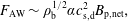 $$\begin{eqnarray}F_{\text{AW}}\sim \unicode[STIX]{x1D70C}_{\text{b}}^{1/2}\unicode[STIX]{x1D6FC}c_{\text{s,d}}^{2}B_{\text{p,net}},\end{eqnarray}$$
where
 $\unicode[STIX]{x1D70C}_{\text{b}}$
is the density at the coronal base. In the
$\unicode[STIX]{x1D70C}_{\text{b}}$
is the density at the coronal base. In the
 $\unicode[STIX]{x1D6FC}$
-disk model, the radiative flux from the disk is
$\unicode[STIX]{x1D6FC}$
-disk model, the radiative flux from the disk is
 $$\begin{eqnarray}q\sim \unicode[STIX]{x1D6FC}\unicode[STIX]{x1D70C}_{\text{d}}c_{\text{s,d}}^{3},\end{eqnarray}$$
where
 $\unicode[STIX]{x1D70C}_{\text{d}}$
is the midplane density. Upon dividing (4.11) by (4.12), we obtain
$\unicode[STIX]{x1D70C}_{\text{d}}$
is the midplane density. Upon dividing (4.11) by (4.12), we obtain
 $$\begin{eqnarray}\frac{F_{\text{AW}}}{q}\sim \left(\frac{\unicode[STIX]{x1D70C}_{\text{b}}}{\unicode[STIX]{x1D70C}_{\text{d}}}\right)^{1/2}\unicode[STIX]{x1D6FD}_{\text{net,d}}^{-1/2},\end{eqnarray}$$
where
 $$\begin{eqnarray}\unicode[STIX]{x1D6FD}_{\text{net}}=\frac{2(p+p_{\text{rad}})}{B_{\text{p,net}}^{2}},\end{eqnarray}$$
and
 $\unicode[STIX]{x1D6FD}_{\text{net,d}}$
is the value of
$\unicode[STIX]{x1D6FD}_{\text{net,d}}$
is the value of
 $\unicode[STIX]{x1D6FD}_{\text{net}}$
at the disk midplane. All quantities in (4.13) are functions of distance
$\unicode[STIX]{x1D6FD}_{\text{net}}$
at the disk midplane. All quantities in (4.13) are functions of distance
 $r$
from the central compact object. Since
$r$
from the central compact object. Since
 $q$
peaks at small
$q$
peaks at small
 $r$
, the ratio of the disk’s AW luminosity to its radiative luminosity is approximately equal to the right-hand side of (4.13) evaluated near the disk’s inner edge.Footnote
3
$r$
, the ratio of the disk’s AW luminosity to its radiative luminosity is approximately equal to the right-hand side of (4.13) evaluated near the disk’s inner edge.Footnote
3
Although (4.13) in principle determines
 $F_{\text{AW}}$
, the factors on the right-hand side of (4.13) have large uncertainties. In numerical simulations of disks,
$F_{\text{AW}}$
, the factors on the right-hand side of (4.13) have large uncertainties. In numerical simulations of disks,
 $\unicode[STIX]{x1D70C}_{\text{b}}/\unicode[STIX]{x1D70C}_{\text{d}}$
ranges from
$\unicode[STIX]{x1D70C}_{\text{b}}/\unicode[STIX]{x1D70C}_{\text{d}}$
ranges from
 $\simeq 10^{-2}$
to
$\simeq 10^{-2}$
to
 $\simeq 0.5$
, depending on a number of factors, including whether radiation pressure dominates over plasma pressure and whether the simulation is local or global (e.g. Jiang, Stone & Davis Reference Jiang, Stone and Davis2014; Jiang, Davis & Stone Reference Jiang, Davis and Stone2016; Zhu & Stone Reference Zhu and Stone2017). The value of
$\simeq 0.5$
, depending on a number of factors, including whether radiation pressure dominates over plasma pressure and whether the simulation is local or global (e.g. Jiang, Stone & Davis Reference Jiang, Stone and Davis2014; Jiang, Davis & Stone Reference Jiang, Davis and Stone2016; Zhu & Stone Reference Zhu and Stone2017). The value of
 $\unicode[STIX]{x1D6FD}_{\text{net,d}}$
depends on the efficiency with which a disk accretes poloidal magnetic flux. A number of studies have argued that if the magnetic field is passively transported by turbulence in the disk and the turbulent diffusion coefficient is uniform, then the time scale for poloidal flux to diffuse outward is shorter than the accretion time scale of the matter (e.g. van Ballegooijen Reference van Ballegooijen and Belvedere1989; Livio, Ogilvie & Pringle Reference Livio, Ogilvie and Pringle1999; Guan & Gammie Reference Guan and Gammie2009; Guilet & Ogilvie Reference Guilet and Ogilvie2013). In this case, little poloidal flux accumulates near the central object, and
$\unicode[STIX]{x1D6FD}_{\text{net,d}}$
depends on the efficiency with which a disk accretes poloidal magnetic flux. A number of studies have argued that if the magnetic field is passively transported by turbulence in the disk and the turbulent diffusion coefficient is uniform, then the time scale for poloidal flux to diffuse outward is shorter than the accretion time scale of the matter (e.g. van Ballegooijen Reference van Ballegooijen and Belvedere1989; Livio, Ogilvie & Pringle Reference Livio, Ogilvie and Pringle1999; Guan & Gammie Reference Guan and Gammie2009; Guilet & Ogilvie Reference Guilet and Ogilvie2013). In this case, little poloidal flux accumulates near the central object, and
 $\unicode[STIX]{x1D6FD}_{\text{net,d}}$
is extremely large. On the other hand, poloidal flux may be dragged inwards much more efficiently if the turbulent diffusion coefficient becomes small near the boundary between the disk and its atmosphere, if the vertical magnetic field in the disk is concentrated into bundles with a small volume filling factor, or if the vertical field exerts significant torque on the disk material (Livio et al.
Reference Livio, Ogilvie and Pringle1999; Spruit & Uzdensky Reference Spruit and Uzdensky2005; Guilet & Ogilvie Reference Guilet and Ogilvie2013). In numerical simulations, if the initial magnetic field is very weak or has toroidally shaped flux surfaces with comparatively small major radii
$\unicode[STIX]{x1D6FD}_{\text{net,d}}$
is extremely large. On the other hand, poloidal flux may be dragged inwards much more efficiently if the turbulent diffusion coefficient becomes small near the boundary between the disk and its atmosphere, if the vertical magnetic field in the disk is concentrated into bundles with a small volume filling factor, or if the vertical field exerts significant torque on the disk material (Livio et al.
Reference Livio, Ogilvie and Pringle1999; Spruit & Uzdensky Reference Spruit and Uzdensky2005; Guilet & Ogilvie Reference Guilet and Ogilvie2013). In numerical simulations, if the initial magnetic field is very weak or has toroidally shaped flux surfaces with comparatively small major radii
 $r_{\text{i}}$
, then little poloidal magnetic flux builds up near the central object (see, e.g. De Villiers, Hawley & Krolik Reference De Villiers, Hawley and Krolik2003b
; Beckwith, Hawley & Krolik Reference Beckwith, Hawley and Krolik2008; McKinney, Tchekhovskoy & Blandford Reference McKinney, Tchekhovskoy and Blandford2012). In contrast, if the initial field is sufficiently strong and
$r_{\text{i}}$
, then little poloidal magnetic flux builds up near the central object (see, e.g. De Villiers, Hawley & Krolik Reference De Villiers, Hawley and Krolik2003b
; Beckwith, Hawley & Krolik Reference Beckwith, Hawley and Krolik2008; McKinney, Tchekhovskoy & Blandford Reference McKinney, Tchekhovskoy and Blandford2012). In contrast, if the initial field is sufficiently strong and
 $r_{\text{i}}$
sufficiently large, or if substantial poloidal magnetic flux is continuously injected into the simulation domain, then poloidal magnetic flux is dragged inwards so efficiently that the outward magnetic pressure force on disk material becomes comparable to the gravitational force, leading to a magnetically arrested disk (Igumenshchev, Narayan & Abramowicz Reference Igumenshchev, Narayan and Abramowicz2003; Tchekhovskoy et al.
Reference Tchekhovskoy, Narayan and McKinney2011).
$r_{\text{i}}$
sufficiently large, or if substantial poloidal magnetic flux is continuously injected into the simulation domain, then poloidal magnetic flux is dragged inwards so efficiently that the outward magnetic pressure force on disk material becomes comparable to the gravitational force, leading to a magnetically arrested disk (Igumenshchev, Narayan & Abramowicz Reference Igumenshchev, Narayan and Abramowicz2003; Tchekhovskoy et al.
Reference Tchekhovskoy, Narayan and McKinney2011).
We note that the ability of turbulent heating to produce a hot corona starting at the
 $\unicode[STIX]{x1D6FD}_{\text{total}}=1$
surface depends not only on
$\unicode[STIX]{x1D6FD}_{\text{total}}=1$
surface depends not only on
 $F_{\text{AW}}$
, but also on the optical depth at this surface,
$F_{\text{AW}}$
, but also on the optical depth at this surface,
 $\unicode[STIX]{x1D70F}_{\text{b}}$
. If
$\unicode[STIX]{x1D70F}_{\text{b}}$
. If
 $\unicode[STIX]{x1D70F}_{\text{b}}\gg 1$
, and if radiative transfer dominates the vertical energy flux above the
$\unicode[STIX]{x1D70F}_{\text{b}}\gg 1$
, and if radiative transfer dominates the vertical energy flux above the
 $\unicode[STIX]{x1D6FD}_{\text{total}}=1$
surface, then the temperature must be a decreasing function of distance from the disk midplane in order to drive an outward radiative energy flux (see, e.g. simulation B of Jiang et al.
Reference Jiang, Stone and Davis2014).
$\unicode[STIX]{x1D6FD}_{\text{total}}=1$
surface, then the temperature must be a decreasing function of distance from the disk midplane in order to drive an outward radiative energy flux (see, e.g. simulation B of Jiang et al.
Reference Jiang, Stone and Davis2014).
4.3 Self-consistency of the RMHD and
$\unicode[STIX]{x1D6FC}$
-disk approximations

One of the assumptions underlying the reduced MHD analysis of §§ 2.3–2.4 is the inequality
 $$\begin{eqnarray}\frac{\langle \unicode[STIX]{x1D6FF}u^{2}\rangle }{v_{\text{A}}^{2}}\ll 1.\end{eqnarray}$$
Close to the coronal base,
 $v_{\text{A}}$
increases with distance from the disk, and we can use (2.28) and (3.8) to rewrite (4.15) as
$v_{\text{A}}$
increases with distance from the disk, and we can use (2.28) and (3.8) to rewrite (4.15) as
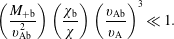 $$\begin{eqnarray}\left(\frac{M_{+\text{b}}}{v_{\text{Ab}}^{2}}\right)\left(\frac{\unicode[STIX]{x1D712}_{\text{b}}}{\unicode[STIX]{x1D712}}\right)\left(\frac{v_{\text{Ab}}}{v_{\text{A}}}\right)^{3}\ll 1.\end{eqnarray}$$
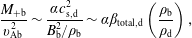 $$\begin{eqnarray}\frac{M_{+\text{b}}}{v_{\text{Ab}}^{2}}\sim \frac{\unicode[STIX]{x1D6FC}c_{\text{s,d}}^{2}}{B_{\text{b}}^{2}/\unicode[STIX]{x1D70C}_{\text{b}}}\sim \unicode[STIX]{x1D6FC}\unicode[STIX]{x1D6FD}_{\text{total,d}}\left(\frac{\unicode[STIX]{x1D70C}_{\text{b}}}{\unicode[STIX]{x1D70C}_{\text{d}}}\right),\end{eqnarray}$$
where
 $B_{\text{b}}$
is the magnetic-field strength at the coronal base, and
$B_{\text{b}}$
is the magnetic-field strength at the coronal base, and
 $\unicode[STIX]{x1D6FD}_{\text{total,d}}$
is the value of
$\unicode[STIX]{x1D6FD}_{\text{total,d}}$
is the value of
 $\unicode[STIX]{x1D6FD}_{\text{total}}$
at the disk midplane. In writing the second order-of-magnitude relationship in (4.17), we have taken the magnetic-field strength to be fairly uniform across the vertical profile of a disk (see, e.g. figure 6 of Beckwith et al. (Reference Beckwith, Hawley and Krolik2008) or figure 2 of Jiang et al. (Reference Jiang, Stone and Davis2014)). The factor of
$\unicode[STIX]{x1D6FD}_{\text{total}}$
at the disk midplane. In writing the second order-of-magnitude relationship in (4.17), we have taken the magnetic-field strength to be fairly uniform across the vertical profile of a disk (see, e.g. figure 6 of Beckwith et al. (Reference Beckwith, Hawley and Krolik2008) or figure 2 of Jiang et al. (Reference Jiang, Stone and Davis2014)). The factor of
 $\unicode[STIX]{x1D6FC}\unicode[STIX]{x1D6FD}_{\text{total,d}}$
in (4.17) is typically one over a few (Blackman, Penna & Varnière Reference Blackman, Penna and Varnière2008; Sorathia et al.
Reference Sorathia, Reynolds, Stone and Beckwith2012; Hawley et al.
Reference Hawley, Richers, Guan and Krolik2013). Since
$\unicode[STIX]{x1D6FC}\unicode[STIX]{x1D6FD}_{\text{total,d}}$
in (4.17) is typically one over a few (Blackman, Penna & Varnière Reference Blackman, Penna and Varnière2008; Sorathia et al.
Reference Sorathia, Reynolds, Stone and Beckwith2012; Hawley et al.
Reference Hawley, Richers, Guan and Krolik2013). Since
 $\unicode[STIX]{x1D70C}_{b}/\unicode[STIX]{x1D70C}_{\text{d}}$
is also less than 1 (or
$\unicode[STIX]{x1D70C}_{b}/\unicode[STIX]{x1D70C}_{\text{d}}$
is also less than 1 (or
 $\ll 1$
),
$\ll 1$
),
 $M_{+\text{b}}/v_{\text{Ab}}^{2}$
is smaller than 1, and (4.16) is at least marginally satisfied at the coronal base. In the low corona, where the flows are at most trans-relativistic and
$M_{+\text{b}}/v_{\text{Ab}}^{2}$
is smaller than 1, and (4.16) is at least marginally satisfied at the coronal base. In the low corona, where the flows are at most trans-relativistic and
 $\overline{{\mathcal{E}}}\sim \overline{\unicode[STIX]{x1D70C}}$
, equation (4.10) implies that
$\overline{{\mathcal{E}}}\sim \overline{\unicode[STIX]{x1D70C}}$
, equation (4.10) implies that
 $$\begin{eqnarray}\left(\frac{\unicode[STIX]{x1D712}_{\text{b}}}{\unicode[STIX]{x1D712}}\right)\left(\frac{v_{\text{Ab}}}{v_{\text{A}}}\right)^{3}\sim \frac{\overline{\unicode[STIX]{x1D70C}}}{\unicode[STIX]{x1D70C}_{\text{b}}}\left(\frac{B_{\text{b}}}{\overline{B}}\right)^{3}.\end{eqnarray}$$
Because the density decreases rapidly with increasing distance
 $h$
from the coronal base in the low disk atmosphere, we expect the right-hand side of (4.18) to decrease with increasing
$h$
from the coronal base in the low disk atmosphere, we expect the right-hand side of (4.18) to decrease with increasing
 $h$
. Thus, not only is (4.16) at least marginally satisfied at the coronal base, but it becomes a better approximation in the low corona. It is possible that the RMHD approximation breaks down at sufficiently large distances from the disk, but whether this happens depends upon the spatial profiles of the background flow and magnetic field. These profiles, in turn, depend upon how much poloidal magnetic flux is accreted towards the central compact object, which, as discussed above, is uncertain.
$h$
. Thus, not only is (4.16) at least marginally satisfied at the coronal base, but it becomes a better approximation in the low corona. It is possible that the RMHD approximation breaks down at sufficiently large distances from the disk, but whether this happens depends upon the spatial profiles of the background flow and magnetic field. These profiles, in turn, depend upon how much poloidal magnetic flux is accreted towards the central compact object, which, as discussed above, is uncertain.
The results of this section are also based upon the
 $\unicode[STIX]{x1D6FC}$
-disk model, in which disk turbulence is the only mechanism for transporting angular momentum away from the central object, and radiation is the only means by which energy escapes from the disk surface. If poloidal magnetic flux is accreted efficiently towards the central compact object and the disk drives a powerful outflow, then the angular momentum flux and energy flux associated with this outflow could modify the disk structure. Our use of the
$\unicode[STIX]{x1D6FC}$
-disk model, in which disk turbulence is the only mechanism for transporting angular momentum away from the central object, and radiation is the only means by which energy escapes from the disk surface. If poloidal magnetic flux is accreted efficiently towards the central compact object and the disk drives a powerful outflow, then the angular momentum flux and energy flux associated with this outflow could modify the disk structure. Our use of the
 $\unicode[STIX]{x1D6FC}$
-disk model thus becomes problematic in the most interesting parameter regime for AW heating, in which
$\unicode[STIX]{x1D6FC}$
-disk model thus becomes problematic in the most interesting parameter regime for AW heating, in which
 $\unicode[STIX]{x1D6FD}_{\text{net,d}}$
is not much greater than 1. If astrophysical disks reach this regime, further work will be needed to model the disks, winds and AW turbulence self-consistently.
$\unicode[STIX]{x1D6FD}_{\text{net,d}}$
is not much greater than 1. If astrophysical disks reach this regime, further work will be needed to model the disks, winds and AW turbulence self-consistently.
5 A sub-grid model for incorporating reflection-driven Alfvén-wave turbulence into numerical simulations of the averaged GRMHD equations
The correlation length of the turbulent fluctuations in a thin accretion disk is smaller than the disk’s thickness. As a consequence, the AWs launched into the corona of a thin disk have a correlation length perpendicular to the magnetic field, as measured in the AFRF in the low atmosphere of the disk, that is smaller than the disk thickness. These AWs cascade to much smaller scales before dissipating and heating the plasma. In order to carry out a direct numerical simulation of the AW turbulence launched from a thin disk into its corona and outflow, it would be necessary to resolve, within the disk’s corona and outflow, length scales much smaller than the disk’s thickness, which is unfeasible even on today’s fastest supercomputers. An alternative approach is to average the GRMHD equations in the manner described in § 2.2, solve these averaged GRMHD equations numerically, and incorporate the mean-square AW amplitude as an additional variable that evolves according to (2.30) and (2.33). In this section, we derive a set of averaged GRMHD equations that can be used in this way.Footnote
4
Throughout this section, we make use of the RMHD orderings of § 2.3 and neglect fluctuations in
 $\unicode[STIX]{x1D70C}$
,
$\unicode[STIX]{x1D70C}$
,
 $u$
(the internal energy) and
$u$
(the internal energy) and
 $p$
.
$p$
.
To begin, we average (2.7) to obtain
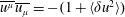 $\overline{u^{\unicode[STIX]{x1D707}}}\overline{u_{\unicode[STIX]{x1D707}}}=-(1+\langle \unicode[STIX]{x1D6FF}u^{2}\rangle )$
. Since
$\overline{u^{\unicode[STIX]{x1D707}}}\overline{u_{\unicode[STIX]{x1D707}}}=-(1+\langle \unicode[STIX]{x1D6FF}u^{2}\rangle )$
. Since
 $\overline{u^{\unicode[STIX]{x1D707}}}\overline{u_{\unicode[STIX]{x1D707}}}\neq -1$
,
$\overline{u^{\unicode[STIX]{x1D707}}}\overline{u_{\unicode[STIX]{x1D707}}}\neq -1$
,
 $\overline{u^{\unicode[STIX]{x1D707}}}$
is not a 4-velocity. On the other hand,
$\overline{u^{\unicode[STIX]{x1D707}}}$
is not a 4-velocity. On the other hand,
 $$\begin{eqnarray}u_{0}^{\unicode[STIX]{x1D707}}=\frac{\overline{u^{\unicode[STIX]{x1D707}}}}{\sqrt{1+\langle \unicode[STIX]{x1D6FF}u^{2}\rangle }}\end{eqnarray}$$
is the 4-velocity of the AFRF, since its spatial components (like those of
 $\overline{u^{\unicode[STIX]{x1D707}}}$
) vanish in the AFRF, and since
$\overline{u^{\unicode[STIX]{x1D707}}}$
) vanish in the AFRF, and since
 $$\begin{eqnarray}u_{0}^{\unicode[STIX]{x1D707}}u_{0\unicode[STIX]{x1D707}}=-1.\end{eqnarray}$$
The mass density of the fluid, as measured by an observer with 4-velocity
 $s^{\unicode[STIX]{x1D707}}$
, is
$s^{\unicode[STIX]{x1D707}}$
, is
 $\unicode[STIX]{x1D6E4}^{\unicode[STIX]{x1D707}}s_{\unicode[STIX]{x1D707}}$
, where
$\unicode[STIX]{x1D6E4}^{\unicode[STIX]{x1D707}}s_{\unicode[STIX]{x1D707}}$
, where
 $\unicode[STIX]{x1D6E4}^{\unicode[STIX]{x1D707}}=\unicode[STIX]{x1D70C}u^{\unicode[STIX]{x1D707}}$
is the mass-flux 4-vector. The averaged mass density measured by an observer at rest in the AFRF is thus
$\unicode[STIX]{x1D6E4}^{\unicode[STIX]{x1D707}}=\unicode[STIX]{x1D70C}u^{\unicode[STIX]{x1D707}}$
is the mass-flux 4-vector. The averaged mass density measured by an observer at rest in the AFRF is thus
 $\unicode[STIX]{x1D70C}_{0}=\langle \unicode[STIX]{x1D6E4}^{\unicode[STIX]{x1D707}}u_{0\unicode[STIX]{x1D707}}\rangle$
, or, equivalently,
$\unicode[STIX]{x1D70C}_{0}=\langle \unicode[STIX]{x1D6E4}^{\unicode[STIX]{x1D707}}u_{0\unicode[STIX]{x1D707}}\rangle$
, or, equivalently,
 $$\begin{eqnarray}\unicode[STIX]{x1D70C}_{0}=\unicode[STIX]{x1D70C}\sqrt{1+\langle \unicode[STIX]{x1D6FF}u^{2}\rangle }.\end{eqnarray}$$
This mass density is larger than the rest-frame density
 $\unicode[STIX]{x1D70C}$
because the fluid moves with respect to the AFRF, and Lorentz contraction causes the apparent density of a moving fluid to be larger than the rest-frame density.
$\unicode[STIX]{x1D70C}$
because the fluid moves with respect to the AFRF, and Lorentz contraction causes the apparent density of a moving fluid to be larger than the rest-frame density.
The magnetic field in the frame of an observer
 $O$
with 4-velocity
$O$
with 4-velocity
 $s^{\unicode[STIX]{x1D707}}$
is
$s^{\unicode[STIX]{x1D707}}$
is
 $B_{(s)}^{\unicode[STIX]{x1D707}}=-(F^{\ast \unicode[STIX]{x1D707}\unicode[STIX]{x1D708}})s_{\unicode[STIX]{x1D708}}$
, where
$B_{(s)}^{\unicode[STIX]{x1D707}}=-(F^{\ast \unicode[STIX]{x1D707}\unicode[STIX]{x1D708}})s_{\unicode[STIX]{x1D708}}$
, where
 $(F^{\ast \unicode[STIX]{x1D707}\unicode[STIX]{x1D708}})=(1/2)\unicode[STIX]{x1D716}^{\unicode[STIX]{x1D707}\unicode[STIX]{x1D708}\unicode[STIX]{x1D705}\unicode[STIX]{x1D70F}}F_{\unicode[STIX]{x1D705}\unicode[STIX]{x1D70F}}=b^{\unicode[STIX]{x1D707}}u^{\unicode[STIX]{x1D708}}-b^{\unicode[STIX]{x1D708}}u^{\unicode[STIX]{x1D707}}$
is the dual of
$(F^{\ast \unicode[STIX]{x1D707}\unicode[STIX]{x1D708}})=(1/2)\unicode[STIX]{x1D716}^{\unicode[STIX]{x1D707}\unicode[STIX]{x1D708}\unicode[STIX]{x1D705}\unicode[STIX]{x1D70F}}F_{\unicode[STIX]{x1D705}\unicode[STIX]{x1D70F}}=b^{\unicode[STIX]{x1D707}}u^{\unicode[STIX]{x1D708}}-b^{\unicode[STIX]{x1D708}}u^{\unicode[STIX]{x1D707}}$
is the dual of
 $F^{\unicode[STIX]{x1D707}\unicode[STIX]{x1D708}}$
. More precisely,
$F^{\unicode[STIX]{x1D707}\unicode[STIX]{x1D708}}$
. More precisely,
 $B_{(s)}^{\unicode[STIX]{x1D707}}$
is that 4-vector which, in the frame of observer O, has a vanishing time component and spatial components equal to the magnetic field that would be measured by O. For example, the magnetic field in the fluid frame is
$B_{(s)}^{\unicode[STIX]{x1D707}}$
is that 4-vector which, in the frame of observer O, has a vanishing time component and spatial components equal to the magnetic field that would be measured by O. For example, the magnetic field in the fluid frame is
 $-(F^{\ast \unicode[STIX]{x1D707}\unicode[STIX]{x1D708}})u_{\unicode[STIX]{x1D708}}=b^{\unicode[STIX]{x1D707}}$
. In the case that
$-(F^{\ast \unicode[STIX]{x1D707}\unicode[STIX]{x1D708}})u_{\unicode[STIX]{x1D708}}=b^{\unicode[STIX]{x1D707}}$
. In the case that
 $g^{tt}=-1$
, the 4-velocity
$g^{tt}=-1$
, the 4-velocity
 $s^{\unicode[STIX]{x1D707}}$
of an observer moving normal to a
$s^{\unicode[STIX]{x1D707}}$
of an observer moving normal to a
 $t=\text{constant}$
‘slice’ satisfies
$t=\text{constant}$
‘slice’ satisfies
 $s_{t}=-1$
and
$s_{t}=-1$
and
 $s_{i}=0$
, and the magnetic field in the frame of this ‘normal observer’ is
$s_{i}=0$
, and the magnetic field in the frame of this ‘normal observer’ is
 $-(F^{\ast \unicode[STIX]{x1D707}\unicode[STIX]{x1D708}})s_{\unicode[STIX]{x1D708}}=(F^{\ast \unicode[STIX]{x1D707}t})=b^{\unicode[STIX]{x1D707}}u^{t}-u^{\unicode[STIX]{x1D707}}b^{t}\equiv B^{\unicode[STIX]{x1D707}}$
(Duez et al.
Reference Duez, Liu, Shapiro and Stephens2005).Footnote
5
The spatial components of
$-(F^{\ast \unicode[STIX]{x1D707}\unicode[STIX]{x1D708}})s_{\unicode[STIX]{x1D708}}=(F^{\ast \unicode[STIX]{x1D707}t})=b^{\unicode[STIX]{x1D707}}u^{t}-u^{\unicode[STIX]{x1D707}}b^{t}\equiv B^{\unicode[STIX]{x1D707}}$
(Duez et al.
Reference Duez, Liu, Shapiro and Stephens2005).Footnote
5
The spatial components of
 $B^{\unicode[STIX]{x1D707}}$
were given in (2.9), and
$B^{\unicode[STIX]{x1D707}}$
were given in (2.9), and
 $B^{t}$
vanishes since
$B^{t}$
vanishes since
 $F^{\ast \unicode[STIX]{x1D707}\unicode[STIX]{x1D708}}$
is antisymmetric. The averaged magnetic field in the AFRF is
$F^{\ast \unicode[STIX]{x1D707}\unicode[STIX]{x1D708}}$
is antisymmetric. The averaged magnetic field in the AFRF is
 $b_{0}^{\unicode[STIX]{x1D707}}=\langle -(F^{\ast \unicode[STIX]{x1D707}\unicode[STIX]{x1D708}})u_{0\unicode[STIX]{x1D708}}\rangle$
, or, equivalently,
$b_{0}^{\unicode[STIX]{x1D707}}=\langle -(F^{\ast \unicode[STIX]{x1D707}\unicode[STIX]{x1D708}})u_{0\unicode[STIX]{x1D708}}\rangle$
, or, equivalently,
 $$\begin{eqnarray}b_{0}^{\unicode[STIX]{x1D707}}=\overline{b^{\unicode[STIX]{x1D707}}}\sqrt{1+\langle \unicode[STIX]{x1D6FF}u^{2}\rangle }-u_{0}^{\unicode[STIX]{x1D707}}\langle \unicode[STIX]{x1D6FF}u^{\unicode[STIX]{x1D6FC}}\unicode[STIX]{x1D6FF}b_{\unicode[STIX]{x1D6FC}}\rangle .\end{eqnarray}$$
Averaging (2.8) yields
 $$\begin{eqnarray}u_{0}^{\unicode[STIX]{x1D707}}b_{0\unicode[STIX]{x1D707}}=0.\end{eqnarray}$$
The continuity and induction equations for the averaged fluid can be obtained by averaging (2.1) and (2.3) and making use of (5.1), (5.3) and (5.4). This yields
 $$\begin{eqnarray}(\unicode[STIX]{x1D70C}_{0}u_{0}^{\unicode[STIX]{x1D708}})_{;\unicode[STIX]{x1D708}}=0\end{eqnarray}$$
and
 $$\begin{eqnarray}\left(u_{0}^{\unicode[STIX]{x1D707}}b_{0}^{\unicode[STIX]{x1D708}}-u_{0}^{\unicode[STIX]{x1D708}}b_{0}^{\unicode[STIX]{x1D707}}\right)_{;\unicode[STIX]{x1D708}}=0.\end{eqnarray}$$
As in § 2.4, we restrict our analysis to the case in which AWs travelling away from the disk have much larger amplitudes than AWs traveling toward the disk in the AFRF. However, in contrast to § 2.4, we here allow either
 $M_{+}$
or
$M_{+}$
or
 $M_{-}$
to correspond to outward-propagating AWs, since in general
$M_{-}$
to correspond to outward-propagating AWs, since in general
 $\overline{B^{i}}$
points toward the disk in some regions and away from the disk in others. We then set
$\overline{B^{i}}$
points toward the disk in some regions and away from the disk in others. We then set
 $$\begin{eqnarray}\unicode[STIX]{x1D6FF}u^{\unicode[STIX]{x1D707}}=\mp \frac{\unicode[STIX]{x1D6FF}b^{\unicode[STIX]{x1D707}}}{\overline{{\mathcal{E}}}^{1/2}},\end{eqnarray}$$
where, here and throughout the remainder of this section, the upper sign corresponds to
 $M_{+}\gg M_{-}$
and the lower sign corresponds to
$M_{+}\gg M_{-}$
and the lower sign corresponds to
 $M_{-}\gg M_{+}$
. Equation (2.28) then becomes
$M_{-}\gg M_{+}$
. Equation (2.28) then becomes
 $$\begin{eqnarray}\langle \unicode[STIX]{x1D6FF}u^{2}\rangle =\frac{M_{\pm }}{4}.\end{eqnarray}$$
Upon averaging
 $T^{\unicode[STIX]{x1D707}\unicode[STIX]{x1D708}}$
, making use of the RMHD orderings described in § 2.3 and dropping terms
$T^{\unicode[STIX]{x1D707}\unicode[STIX]{x1D708}}$
, making use of the RMHD orderings described in § 2.3 and dropping terms
 $\ll \unicode[STIX]{x1D716}^{2}v_{\text{A}}^{2}\overline{{\mathcal{E}}}$
, we obtain
$\ll \unicode[STIX]{x1D716}^{2}v_{\text{A}}^{2}\overline{{\mathcal{E}}}$
, we obtain
 $$\begin{eqnarray}\langle T^{\unicode[STIX]{x1D707}\unicode[STIX]{x1D708}}\rangle =T_{0}^{\unicode[STIX]{x1D707}\unicode[STIX]{x1D708}}+T_{2}^{\unicode[STIX]{x1D707}\unicode[STIX]{x1D708}},\end{eqnarray}$$
where
 $$\begin{eqnarray}\displaystyle & \displaystyle T_{0}^{\unicode[STIX]{x1D707}\unicode[STIX]{x1D708}}={\mathcal{E}}_{0}u_{0}^{\unicode[STIX]{x1D707}}u_{0}^{\unicode[STIX]{x1D708}}+\left(p+\frac{b_{0}^{2}}{2}\right)g^{\unicode[STIX]{x1D707}\unicode[STIX]{x1D708}}-b_{0}^{\unicode[STIX]{x1D707}}b_{0}^{\unicode[STIX]{x1D708}}, & \displaystyle\end{eqnarray}$$
 $$\begin{eqnarray}\displaystyle & \displaystyle T_{2}^{\unicode[STIX]{x1D707}\unicode[STIX]{x1D708}}={\mathcal{E}}_{0}\langle \unicode[STIX]{x1D6FF}u^{2}\rangle \left[\left(2-v_{\text{A0}}^{2}-\frac{\unicode[STIX]{x1D70C}_{0}}{2{\mathcal{E}}_{0}}\right)u_{0}^{\unicode[STIX]{x1D707}}u_{0}^{\unicode[STIX]{x1D708}}+\left(\frac{1-v_{\text{A0}}^{2}}{2}\right)g^{\unicode[STIX]{x1D707}\unicode[STIX]{x1D708}}+v_{\text{A0}}^{\unicode[STIX]{x1D707}}v_{\text{A0}}^{\unicode[STIX]{x1D708}}\pm u_{0}^{\unicode[STIX]{x1D707}}v_{\text{A0}}^{\unicode[STIX]{x1D708}}\pm u_{0}^{\unicode[STIX]{x1D708}}v_{\text{A0}}^{\unicode[STIX]{x1D707}}\right], & \displaystyle \nonumber\\ \displaystyle & & \displaystyle\end{eqnarray}$$
and
 $$\begin{eqnarray}{\mathcal{E}}_{0}\equiv \unicode[STIX]{x1D70C}_{0}+u+p+b_{0}^{2}\qquad v_{\text{A0}}^{\unicode[STIX]{x1D707}}=b_{0}^{\unicode[STIX]{x1D707}}/{\mathcal{E}}_{0}^{1/2}.\end{eqnarray}$$
The average of (2.2), combined with (5.10), yields
 $$\begin{eqnarray}T_{0\;\;\;\,;\unicode[STIX]{x1D708}}^{\unicode[STIX]{x1D707}\unicode[STIX]{x1D708}}=-T_{2\;\;\;\,;\unicode[STIX]{x1D708}}^{\unicode[STIX]{x1D707}\unicode[STIX]{x1D708}}.\end{eqnarray}$$
Equations (2.30), (2.33), (5.5), (5.6), (5.7) and (5.14), along with an equation of state
 $p=p(u,\unicode[STIX]{x1D70C})$
, can be solved for
$p=p(u,\unicode[STIX]{x1D70C})$
, can be solved for
 $\unicode[STIX]{x1D70C}_{0}$
,
$\unicode[STIX]{x1D70C}_{0}$
,
 $u_{0}^{\unicode[STIX]{x1D707}}$
,
$u_{0}^{\unicode[STIX]{x1D707}}$
,
 $b_{0}^{\unicode[STIX]{x1D707}}$
,
$b_{0}^{\unicode[STIX]{x1D707}}$
,
 $u$
,
$u$
,
 $p$
and
$p$
and
 $M_{\pm }$
(with the proviso that if
$M_{\pm }$
(with the proviso that if
 $M_{-}\gg M_{+}$
, then the plus and minus subscripts need to be interchanged in (2.30) and (2.33)). In this closed system of equations, the AW fluctuations are treated like a fluid that co-evolves with the plasma, and all quantities, including
$M_{-}\gg M_{+}$
, then the plus and minus subscripts need to be interchanged in (2.30) and (2.33)). In this closed system of equations, the AW fluctuations are treated like a fluid that co-evolves with the plasma, and all quantities, including
 $M_{\pm }$
, vary on the length scale
$M_{\pm }$
, vary on the length scale
 $L$
of the background flow, which greatly exceeds the perpendicular correlation length
$L$
of the background flow, which greatly exceeds the perpendicular correlation length
 $\unicode[STIX]{x03BB}$
of the fluctuations. The effects of turbulent heating and momentum deposition are captured by the source term
$\unicode[STIX]{x03BB}$
of the fluctuations. The effects of turbulent heating and momentum deposition are captured by the source term
 $-T_{2\;\;\;\,;\unicode[STIX]{x1D708}}^{\unicode[STIX]{x1D707}\unicode[STIX]{x1D708}}$
on the right-hand side of (5.14). Since this source term contains time derivatives, some care is needed when adding it to a GRMHD code. The development of an appropriate numerical algorithm, however, lies beyond the scope of this paper.
$-T_{2\;\;\;\,;\unicode[STIX]{x1D708}}^{\unicode[STIX]{x1D707}\unicode[STIX]{x1D708}}$
on the right-hand side of (5.14). Since this source term contains time derivatives, some care is needed when adding it to a GRMHD code. The development of an appropriate numerical algorithm, however, lies beyond the scope of this paper.
If we ignore, for the moment, dissipation of AW turbulence and consider the ideal GRMHD equations, contracting (2.2) with
 $u_{\unicode[STIX]{x1D707}}$
yields
$u_{\unicode[STIX]{x1D707}}$
yields
 $(u^{\unicode[STIX]{x1D708}}u)_{;\unicode[STIX]{x1D708}}+pu_{;\unicode[STIX]{x1D708}}^{\unicode[STIX]{x1D708}}=0$
, which implies that the specific entropy of each fluid element is an invariant (Anile Reference Anile1989). For example, if
$(u^{\unicode[STIX]{x1D708}}u)_{;\unicode[STIX]{x1D708}}+pu_{;\unicode[STIX]{x1D708}}^{\unicode[STIX]{x1D708}}=0$
, which implies that the specific entropy of each fluid element is an invariant (Anile Reference Anile1989). For example, if
 $p$
were simply
$p$
were simply
 $(\unicode[STIX]{x1D6FE}-1)u$
for some constant
$(\unicode[STIX]{x1D6FE}-1)u$
for some constant
 $\unicode[STIX]{x1D6FE}$
, then
$\unicode[STIX]{x1D6FE}$
, then
 $u^{\unicode[STIX]{x1D708}}\unicode[STIX]{x2202}_{\unicode[STIX]{x1D708}}\ln (p/\unicode[STIX]{x1D70C}^{\unicode[STIX]{x1D6FE}})=0$
(Del Zanna et al.
Reference Del Zanna, Zanotti, Bucciantini and Londrillo2007). However, the dissipation of AW turbulence, which is modelled by the
$u^{\unicode[STIX]{x1D708}}\unicode[STIX]{x2202}_{\unicode[STIX]{x1D708}}\ln (p/\unicode[STIX]{x1D70C}^{\unicode[STIX]{x1D6FE}})=0$
(Del Zanna et al.
Reference Del Zanna, Zanotti, Bucciantini and Londrillo2007). However, the dissipation of AW turbulence, which is modelled by the
 $-2\unicode[STIX]{x1D6FE}_{+}M_{+}$
term on the right-hand side of (2.30), should lead to entropy production, i.e. heating. To see how such heating results from (5.14), we contract (5.14) with
$-2\unicode[STIX]{x1D6FE}_{+}M_{+}$
term on the right-hand side of (2.30), should lead to entropy production, i.e. heating. To see how such heating results from (5.14), we contract (5.14) with
 $\overline{u_{\unicode[STIX]{x1D707}}}$
, add (2.30) times
$\overline{u_{\unicode[STIX]{x1D707}}}$
, add (2.30) times
 ${\mathcal{E}}_{0}/4$
, and drop terms that are
${\mathcal{E}}_{0}/4$
, and drop terms that are
 $\ll \unicode[STIX]{x1D716}^{2}{\mathcal{E}}v_{A}^{3}/L$
, obtaining
$\ll \unicode[STIX]{x1D716}^{2}{\mathcal{E}}v_{A}^{3}/L$
, obtaining
 $$\begin{eqnarray}(\overline{u^{\unicode[STIX]{x1D708}}}u)_{;\unicode[STIX]{x1D708}}+p\overline{u^{\unicode[STIX]{x1D708}}}_{;\unicode[STIX]{x1D708}}=\frac{\unicode[STIX]{x1D6FE}_{\pm }\overline{{\mathcal{E}}}M_{\pm }}{2},\end{eqnarray}$$
where it is
 $\overline{u^{\unicode[STIX]{x1D708}}}$
rather than
$\overline{u^{\unicode[STIX]{x1D708}}}$
rather than
 $u_{0}^{\unicode[STIX]{x1D708}}$
that appears in (5.15). (The
$u_{0}^{\unicode[STIX]{x1D708}}$
that appears in (5.15). (The
 $\overline{{\mathcal{E}}}$
on the right-hand side is interchangeable with
$\overline{{\mathcal{E}}}$
on the right-hand side is interchangeable with
 ${\mathcal{E}}_{0}$
to the order of accuracy of the equation.) We identify the right-hand side of (5.15) as the turbulent heating rate, which was previously stated in (2.34) for the case
${\mathcal{E}}_{0}$
to the order of accuracy of the equation.) We identify the right-hand side of (5.15) as the turbulent heating rate, which was previously stated in (2.34) for the case
 $M_{+}\gg M_{-}$
.
$M_{+}\gg M_{-}$
.
6 Summary and conclusion
We investigate the propagation, reflection and nonlinear evolution of AWs launched from a turbulent accretion disk. We focus on open-field regions, in which the magnetic-field lines extend from the disk’s surface, through the corona and into an overlying outflow. Working within the framework of GRMHD, we derive a set of equations that can be solved for the mean-square AW amplitude and turbulent heating rate as functions of position, and we solve these equations analytically for the case of a time-independent and axisymmetric background flow. Applying these results to the corona and outflow above a thin
 $\unicode[STIX]{x1D6FC}$
-disk, we show that the AW energy flux from the disk is approximately
$\unicode[STIX]{x1D6FC}$
-disk, we show that the AW energy flux from the disk is approximately
 $(\unicode[STIX]{x1D70C}_{\text{b}}/\unicode[STIX]{x1D70C}_{\text{d}})^{1/2}\unicode[STIX]{x1D6FD}_{\text{net,d}}^{-1/2}$
times the disk’s radiative flux, where
$(\unicode[STIX]{x1D70C}_{\text{b}}/\unicode[STIX]{x1D70C}_{\text{d}})^{1/2}\unicode[STIX]{x1D6FD}_{\text{net,d}}^{-1/2}$
times the disk’s radiative flux, where
 $\unicode[STIX]{x1D70C}_{\text{b}}$
and
$\unicode[STIX]{x1D70C}_{\text{b}}$
and
 $\unicode[STIX]{x1D70C}_{\text{d}}$
are the densities at the coronal base and disk midplane, respectively, and
$\unicode[STIX]{x1D70C}_{\text{d}}$
are the densities at the coronal base and disk midplane, respectively, and
 $\unicode[STIX]{x1D6FD}_{\text{net,d}}$
is the ratio (evaluated at the disk midplane) of plasma-plus-radiation pressure to the pressure of the average vertical magnetic field. We also derive a set of averaged GRMHD equations that describe the evolution of the background flow in the presence of reflection-driven AW turbulence.
$\unicode[STIX]{x1D6FD}_{\text{net,d}}$
is the ratio (evaluated at the disk midplane) of plasma-plus-radiation pressure to the pressure of the average vertical magnetic field. We also derive a set of averaged GRMHD equations that describe the evolution of the background flow in the presence of reflection-driven AW turbulence.
A general feature of reflection-driven AW turbulence is that, as AWs propagate away from the disk into regions with varying values of
 $v_{\text{A}}$
, a significant fraction of the AW energy cascades and dissipates each time
$v_{\text{A}}$
, a significant fraction of the AW energy cascades and dissipates each time
 $v_{\text{A}}$
changes by a factor of
$v_{\text{A}}$
changes by a factor of
 ${\sim}2$
. As a consequence, much of the AW energy launched by an accretion disk cascades and dissipates within a few Alfvén-speed scale heights of the disk. This makes AW turbulence a promising mechanism for explaining the compact X-ray emitting coronae that are observed around a number of luminous AGN.
${\sim}2$
. As a consequence, much of the AW energy launched by an accretion disk cascades and dissipates within a few Alfvén-speed scale heights of the disk. This makes AW turbulence a promising mechanism for explaining the compact X-ray emitting coronae that are observed around a number of luminous AGN.
In addition to generating compact AGN coronae, AW heating could have a number of consequences for astrophysical disks, coronae and jets. AW heating increases the density scale height in a disk’s atmosphere, which enhances the mass outflow rate from the disk and reduces the near-BH mass supply. By loading more mass onto the magnetic-field lines above an accretion disk, AW heating could increase the mechanical luminosity of outflows driven by large-scale magnetic forces. If AW heating deposits substantial energy into the outflowing material far from the disk, this heating could lead to faster outflows (cf. Leer & Holzer Reference Leer and Holzer1980). If AWs in the corona (where
 $\unicode[STIX]{x1D6FD}_{\text{total}}\ll 1$
) mostly heat electrons (Quataert Reference Quataert1998; Quataert & Gruzinov Reference Quataert and Gruzinov1999; Howes Reference Howes2010; Ressler et al.
Reference Ressler, Tchekhovskoy, Quataert, Chandra and Gammie2015, Reference Ressler, Tchekhovskoy, Quataert and Gammie2017), then AW dissipation could lead to substantial coronal emission. Particle-in-cell simulations show that turbulence in relativistic pair plasmas can lead to a power-law tail in the particle energy distribution (Zhdankin et al.
Reference Zhdankin, Werner, Uzdensky and Begelman2017), which raises the possibility that AW turbulence in disk coronae and outflows could be an important source of energetic particles. Thermal conduction from the corona into a thin disk may in some cases lead to the evaporation of the disk (Meyer & Meyer-Hofmeister Reference Meyer and Meyer-Hofmeister1994) and the long-sought ‘soft-to-hard’ state transition, in which a thin disk inflates, becoming a thick disk. Conversely, if the density of a thick disk of thickness
$\unicode[STIX]{x1D6FD}_{\text{total}}\ll 1$
) mostly heat electrons (Quataert Reference Quataert1998; Quataert & Gruzinov Reference Quataert and Gruzinov1999; Howes Reference Howes2010; Ressler et al.
Reference Ressler, Tchekhovskoy, Quataert, Chandra and Gammie2015, Reference Ressler, Tchekhovskoy, Quataert and Gammie2017), then AW dissipation could lead to substantial coronal emission. Particle-in-cell simulations show that turbulence in relativistic pair plasmas can lead to a power-law tail in the particle energy distribution (Zhdankin et al.
Reference Zhdankin, Werner, Uzdensky and Begelman2017), which raises the possibility that AW turbulence in disk coronae and outflows could be an important source of energetic particles. Thermal conduction from the corona into a thin disk may in some cases lead to the evaporation of the disk (Meyer & Meyer-Hofmeister Reference Meyer and Meyer-Hofmeister1994) and the long-sought ‘soft-to-hard’ state transition, in which a thin disk inflates, becoming a thick disk. Conversely, if the density of a thick disk of thickness
 $H\sim c_{\text{s,d}}/\unicode[STIX]{x1D6FA}$
increases sufficiently that radiative cooling causes the disk to collapse parallel to the spin axis to form a thin disk, then
$H\sim c_{\text{s,d}}/\unicode[STIX]{x1D6FA}$
increases sufficiently that radiative cooling causes the disk to collapse parallel to the spin axis to form a thin disk, then
 $\unicode[STIX]{x1D6FD}_{\text{net,d}}\propto \unicode[STIX]{x1D70C}_{\text{d}}c_{\text{ s,d}}^{2}/B_{\text{p,net}}^{2}\propto H/B_{\text{p,net}}^{2}$
decreases during the collapse (since neither
$\unicode[STIX]{x1D6FD}_{\text{net,d}}\propto \unicode[STIX]{x1D70C}_{\text{d}}c_{\text{ s,d}}^{2}/B_{\text{p,net}}^{2}\propto H/B_{\text{p,net}}^{2}$
decreases during the collapse (since neither
 $B_{\text{p,net}}$
nor
$B_{\text{p,net}}$
nor
 $\unicode[STIX]{x1D70C}_{\text{d}}H$
changes during the collapse), and there may be a transient period (terminated, e.g. by outward diffusion of poloidal magnetic flux) in which the AW luminosity is strongly enhanced.
$\unicode[STIX]{x1D70C}_{\text{d}}H$
changes during the collapse), and there may be a transient period (terminated, e.g. by outward diffusion of poloidal magnetic flux) in which the AW luminosity is strongly enhanced.
Finally, we note that in current numerical simulations of thin disks, AW turbulence on length scales
 ${<}H$
is under-resolved and significantly modified by numerical dissipation. Moreover, since disk coronae are nearly collisionless, the AW energy that is dissipated in a disk’s corona is partitioned between electrons and protons in a way that cannot be determined within the framework of MHD. Further studies aimed at capturing the AW heating process and its differential effects on protons and electrons, either analytically or through the use of sub-grid models in numerical simulations, will be needed in order to determine the impact of AW heating on disk winds and jets.
${<}H$
is under-resolved and significantly modified by numerical dissipation. Moreover, since disk coronae are nearly collisionless, the AW energy that is dissipated in a disk’s corona is partitioned between electrons and protons in a way that cannot be determined within the framework of MHD. Further studies aimed at capturing the AW heating process and its differential effects on protons and electrons, either analytically or through the use of sub-grid models in numerical simulations, will be needed in order to determine the impact of AW heating on disk winds and jets.
Acknowledgements
We thank E. Blackman for helpful discussions about turbulence in
 $\unicode[STIX]{x1D6FC}$
disks and the anonymous referee for comments that led to improvements in the manuscript. This work was supported in part by NASA grants NNX15AI80, NNX16AG81G and NNX17AI18G and NSF grant PHY-1500041. F.F.’s participation in this work was supported by NASA through Einstein Postdoctoral Fellowship grant number PF4-150122 awarded by the Chandra X-ray Center, which is operated by the Smithsonian Astrophysical Observatory for NASA under contract NAS8-03060. A.T.’s participation in this work was supported by a TAC Fellowship at the University of California, Berkeley.
$\unicode[STIX]{x1D6FC}$
disks and the anonymous referee for comments that led to improvements in the manuscript. This work was supported in part by NASA grants NNX15AI80, NNX16AG81G and NNX17AI18G and NSF grant PHY-1500041. F.F.’s participation in this work was supported by NASA through Einstein Postdoctoral Fellowship grant number PF4-150122 awarded by the Chandra X-ray Center, which is operated by the Smithsonian Astrophysical Observatory for NASA under contract NAS8-03060. A.T.’s participation in this work was supported by a TAC Fellowship at the University of California, Berkeley.
Appendix A. The statistically steady, axisymmetric case
In this appendix, we derive (3.6) and (3.7) starting from (2.30) under the assumption that the background flow is time independent and axisymmetric. Given this assumption, the average of (2.1) leads to
 $$\begin{eqnarray}\overline{u^{\unicode[STIX]{x1D708}}}_{;\unicode[STIX]{x1D708}}=-\overline{u^{\unicode[STIX]{x1D708}}}\unicode[STIX]{x2202}_{\unicode[STIX]{x1D708}}\ln \overline{\unicode[STIX]{x1D70C}}=-u_{\text{p}}^{i}\unicode[STIX]{x2202}_{i}\ln \overline{\unicode[STIX]{x1D70C}},\end{eqnarray}$$
where we have neglected density fluctuations because of the reduced-MHD orderings in (2.18). With the use of (2.11), (3.2), (3.3) and (3.4), we obtain
 $$\begin{eqnarray}\overline{v_{\text{A}}^{\unicode[STIX]{x1D708}}}_{;\unicode[STIX]{x1D708}}=\frac{1}{\sqrt{-g}}\,\unicode[STIX]{x2202}_{i}\left(\frac{\sqrt{-g}\,\unicode[STIX]{x1D702}B_{\text{p}}^{i}}{\overline{{\mathcal{E}}}^{1/2}}\right)=B_{\text{p}}^{i}\unicode[STIX]{x2202}_{i}\left(\frac{\unicode[STIX]{x1D702}}{\overline{{\mathcal{E}}}^{1/2}}\right)=yu_{\text{p}}^{i}\left(\unicode[STIX]{x2202}_{i}\ln \unicode[STIX]{x1D702}-\frac{1}{2}\unicode[STIX]{x2202}_{i}\ln \overline{{\mathcal{E}}}\right).\end{eqnarray}$$
Equations (3.4), (A 1) and (A 2) allow us to rewrite (2.30) in the form
 $$\begin{eqnarray}(1+y)u_{\text{p}}^{i}\unicode[STIX]{x2202}_{i}\ln M_{+}+u_{\text{p}}^{i}\left[-2\unicode[STIX]{x2202}_{i}\ln \overline{\unicode[STIX]{x1D70C}}+\left(\frac{3}{2}+\frac{y}{2}\right)\unicode[STIX]{x2202}_{i}\ln \overline{{\mathcal{E}}}+2y\unicode[STIX]{x2202}_{i}\ln \unicode[STIX]{x1D702}\right]=-2\unicode[STIX]{x1D6FE}_{+}.\end{eqnarray}$$
To solve (A 3), we search for an integrating factor
 $\unicode[STIX]{x1D712}$
that satisfies the equation
$\unicode[STIX]{x1D712}$
that satisfies the equation
 $$\begin{eqnarray}(1+y)u_{\text{p}}^{i}\unicode[STIX]{x2202}_{i}\ln \unicode[STIX]{x1D712}=u_{\text{p}}^{i}\left[-2\unicode[STIX]{x2202}_{i}\ln \overline{\unicode[STIX]{x1D70C}}+\left(\frac{3}{2}+\frac{y}{2}\right)\unicode[STIX]{x2202}_{i}\ln \overline{{\mathcal{E}}}+2y\unicode[STIX]{x2202}_{i}\ln \unicode[STIX]{x1D702}\right].\end{eqnarray}$$
If we can find such an integrating factor, then we can combine (A 3) and (A 4) and, making use of (3.4), obtain
 $$\begin{eqnarray}(u_{\text{p}}^{i}+v_{\text{Ap}}^{i})\unicode[STIX]{x2202}_{i}\ln (\unicode[STIX]{x1D712}M_{+})=-2\unicode[STIX]{x1D6FE}_{+},\end{eqnarray}$$
which is equivalent to (3.6).
To solve (A 4), we first simplify notation, defining
 $$\begin{eqnarray}\displaystyle A=u_{\text{p}}^{i}\unicode[STIX]{x2202}_{i}\ln \overline{\unicode[STIX]{x1D70C}}, & & \displaystyle\end{eqnarray}$$
 $$\begin{eqnarray}\displaystyle C=u_{\text{p}}^{i}\unicode[STIX]{x2202}_{i}\ln \overline{{\mathcal{E}}}, & & \displaystyle\end{eqnarray}$$
and
 $$\begin{eqnarray}D=u_{\text{p}}^{i}\unicode[STIX]{x2202}_{i}\ln \unicode[STIX]{x1D702},\end{eqnarray}$$
so that (A 4) becomes
 $$\begin{eqnarray}(1+y)u_{\text{p}}^{i}\unicode[STIX]{x2202}_{i}\ln \unicode[STIX]{x1D712}=-2A+\left(\frac{3}{2}+\frac{y}{2}\right)C+2yD.\end{eqnarray}$$
We note that
 $$\begin{eqnarray}u_{\text{p}}^{i}\unicode[STIX]{x2202}_{i}\ln y=A-\frac{C}{2}+D\end{eqnarray}$$
and
 $$\begin{eqnarray}-2A+\left(\frac{3}{2}+\frac{y}{2}\right)C+2yD=\left(A-\frac{C}{2}+D\right)(y-1)+\left(-A+C+D\right)(y+1).\end{eqnarray}$$
Substituting (A 10) and (A 11) into (A 9) and dividing by
 $y+1$
, we obtain
$y+1$
, we obtain
 $$\begin{eqnarray}u_{\text{p}}^{i}\unicode[STIX]{x2202}_{i}\ln \unicode[STIX]{x1D712}=\left(\frac{y-1}{y+1}\right)u_{\text{p}}^{i}\unicode[STIX]{x2202}_{i}\ln y-A+C+D,\end{eqnarray}$$
or, equivalently,
 $$\begin{eqnarray}u_{\text{p}}^{i}\unicode[STIX]{x2202}_{i}\ln \unicode[STIX]{x1D712}=u_{\text{p}}^{i}\unicode[STIX]{x2202}_{i}\ln \left[\frac{(y+1)^{2}}{y}\right]-u_{\text{p}}^{i}\unicode[STIX]{x2202}_{i}\ln \overline{\unicode[STIX]{x1D70C}}+u_{\text{p}}^{i}\unicode[STIX]{x2202}_{i}\ln \overline{{\mathcal{E}}}+u_{\text{p}}^{i}\unicode[STIX]{x2202}_{i}\ln \unicode[STIX]{x1D702}.\end{eqnarray}$$
Equation (A 13) can be immediately integrated to yield
 $$\begin{eqnarray}\unicode[STIX]{x1D712}=\unicode[STIX]{x1D713}\times \frac{(y+1)^{2}\overline{{\mathcal{E}}}\unicode[STIX]{x1D702}}{y\overline{\unicode[STIX]{x1D70C}}},\end{eqnarray}$$
where
 $\unicode[STIX]{x1D713}$
is any quantity that is constant along the lines of flow and force:
$\unicode[STIX]{x1D713}$
is any quantity that is constant along the lines of flow and force:
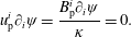 $$\begin{eqnarray}u_{\text{p}}^{i}\unicode[STIX]{x2202}_{i}\unicode[STIX]{x1D713}=\frac{B_{\text{p}}^{i}\unicode[STIX]{x2202}_{i}\unicode[STIX]{x1D713}}{\unicode[STIX]{x1D705}}=0.\end{eqnarray}$$
We set
 $\unicode[STIX]{x1D713}=1/\unicode[STIX]{x1D705}\overline{\unicode[STIX]{x1D70C}}$
, which satisfies (A 15) given (3.3). Equations (3.4) and (3.5) then enable us to set
$\unicode[STIX]{x1D713}=1/\unicode[STIX]{x1D705}\overline{\unicode[STIX]{x1D70C}}$
, which satisfies (A 15) given (3.3). Equations (3.4) and (3.5) then enable us to set
 $\unicode[STIX]{x1D713}\overline{{\mathcal{E}}}\unicode[STIX]{x1D702}/(y\overline{\unicode[STIX]{x1D70C}})=\overline{{\mathcal{E}}}^{3/2}/\overline{\unicode[STIX]{x1D70C}}^{2}$
and
$\unicode[STIX]{x1D713}\overline{{\mathcal{E}}}\unicode[STIX]{x1D702}/(y\overline{\unicode[STIX]{x1D70C}})=\overline{{\mathcal{E}}}^{3/2}/\overline{\unicode[STIX]{x1D70C}}^{2}$
and
 $(1+y)^{2}=(u_{\text{p}}+v_{\text{Ap}})^{2}/u_{\text{p}}^{2}$
in (A 14), which yields (3.7).
$(1+y)^{2}=(u_{\text{p}}+v_{\text{Ap}})^{2}/u_{\text{p}}^{2}$
in (A 14), which yields (3.7).


