Hostname: page-component-78c5997874-t5tsf Total loading time: 0 Render date: 2024-11-19T03:11:31.234Z Has data issue: false hasContentIssue false

A simple analytical model for turbulent kinetic energy dissipation for self-similar round turbulent jets

Published online by Cambridge University Press:  25 March 2024
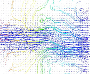
Gagan Kewalramani*
Affiliation:
Université de Lorraine, CNRS, LEMTA, F-54000, Nancy, France
Bowen Ji
Affiliation:
Université de Lorraine, CNRS, LEMTA, F-54000, Nancy, France
Yvan Dossmann
Affiliation:
Université de Lorraine, CNRS, LEMTA, F-54000, Nancy, France
Simon Becker
Affiliation:
Université de Lorraine, CNRS, LEMTA, F-54000, Nancy, France
Michel Gradeck
Affiliation:
Université de Lorraine, CNRS, LEMTA, F-54000, Nancy, France
Nicolas Rimbert
Affiliation:
Université de Lorraine, CNRS, LEMTA, F-54000, Nancy, France
*
Email address for correspondence: [email protected]

Abstract

This work presents a simple analytical model for the streamwise and radial variations of turbulent kinetic energy dissipation in an incompressible round turbulent jet. The key assumptions in the model are: similarity in the axial velocity profile with a Gaussian shape, axisymmetric flow and the dominance of radial derivatives of the mean velocity over axial direction derivatives (similar to boundary layer theory). Initially, a simplified eddy-viscosity relation for turbulent stresses is derived using the algebraic stress model by Gatski & Speziale (J. Fluid Mech., vol. 254, 1993, pp. 59–78). Subsequently, with this eddy-viscosity relation, the relation for variations of turbulent kinetic energy dissipation is formulated using the conservation of turbulent kinetic energy. To extract the necessary constants of the model, experimental velocity statistics for round jets are obtained through particle image velocimetry measurements. The experimental results of the mean entrainment coefficient for turbulent jets are also analysed. When comparing the radial variation of turbulent kinetic energy dissipation from the model with experimental results at Reynolds number $1.4\times 10^5$ and numerical results at Reynolds number $1200$ from the available literature, we observe a maximum error of $10\,\%$ and $15\,\%$, respectively. Finally, using the validated model, we analyse the impact of mean velocity evolution parameters on the behaviour of turbulent kinetic energy dissipation and discuss its potential significance in future studies.

JFM classification

Type
JFM Papers
Copyright
© The Author(s), 2024. Published by Cambridge University Press

1. Introduction and related literature

Turbulent jets are a canonical example of non-homogeneous turbulent flows having environmental and industrial applications. Although single-phase turbulent jets are inhomogeneous and anisotropic flows, the simplifying feature of single-phase jet flow is self-similarity i.e. similar shape of scaled mean and fluctuating velocities. The self-similarity in turbulent jets is observed usually after an axial distance of 15 times the diameter ($D$) from the inlet. Interestingly for jets, the self-similarity is observed irrespective of injecting nozzle conditions, as reported by Breda & Buxton (Reference Breda and Buxton2018) and Ball, Fellouah & Pollard (Reference Ball, Fellouah and Pollard2012). In the self-similar region, a linear variation of the spreading rate and centreline velocity decay rate is assumed with the help of virtual origin correction. The self-similarity in jets is a result of an equilibrium between mean velocity and turbulent fluctuations. This equilibrium is such that the anisotropy and inhomogeneity in fluctuations are sustained by the radial spreading of the mean flow. Such behaviour in turbulent jets can provide some simplification to analyse non-homogeneous and non-isotropic turbulence in jets. To understand the turbulence in jets with different levels of inhomogeneity, it is important to characterize turbulent dissipation at various radial locations starting from the centreline (with nearly homogeneous flow) to the turbulent/non-turbulent interface of the jet. Thus, a simple model for the radial variation of turbulent kinetic energy dissipation is developed in the present work. A brief review of scaling for turbulent kinetic energy dissipation with its importance for large eddy simulation and turbulence modelling is presented by Vassilicos (Reference Vassilicos2015).

Various studies in the literature for the self-similar behaviour of turbulent kinetic energy ($k$) and its dissipation ($\bar {\epsilon }$) at the centreline of the jet are presented hereafter. One of the initial studies for $\bar {\epsilon }$ in jets was performed by George (Reference George1989) by using self-preservation scaling. George (Reference George1989) used the turbulent kinetic energy evolution equation, simplified it using the self-preservation of each term and obtained an expression for the functional form of dissipation. With a similar procedure, Burattini, Antonia & Danaila (Reference Burattini, Antonia and Danaila2005) proposed a self-similar analysis of dissipation by using the two-point structure function equation (i.e. using generalized Kolmogorov relations) for turbulent kinetic energy. Later, Thiesset, Antonia & Djenidi (Reference Thiesset, Antonia and Djenidi2014), using the Kolmogorov velocity and length scale as similarity variables in the equation for the second-order turbulence structure function, obtained a scaling of $\bar {\epsilon } \sim y^{-4}$ (here, $y$ is the normalized axial distance) and its prefactor. However, Sadeghi, Lavoie & Pollard (Reference Sadeghi, Lavoie and Pollard2015), using a similar formulation and scaling it with the Taylor micro-scale, obtained a power law of scaling as $\bar {\epsilon } \sim m y^{m-2}$ (here, $m$ is the power law scaling exponent of $k$). Recently, Viggiano et al. (Reference Viggiano, Basset, Solovitz, Barois, Gibert, Mordant, Chevillard, Volk, Bourgoin and Cal2021), using Lagrangian trajectory results in the self-similar region of turbulent jets, also reported $\bar {\epsilon } \sim y^{-4}$. For a turbulent jet, self-similarity of the velocity correlation was also reported by Ewing et al. (Reference Ewing, Frohnapfel, George, Pedersen and Westerweel2007), however, it was also observed that this similarity in velocity correlation is not independent of the spreading rate.

Most of the analysis stated in the literature is based on two important assumptions: (i) complete self-similarity of various terms and (ii) constant mean axial momentum causing a linear spreading rate. These assumptions may not be universal for all jets. For instance, recent experimental results by Breda & Buxton (Reference Breda and Buxton2018) have observed a weak self-similarity (instead of complete self-similarity) of $\bar {\epsilon }$ until a distance of 30 times the diameter. Also, the approximation of constant mean momentum may not hold appropriately in flows such as plumes or sprays. Therefore, in the present study, we present a simple model to analyse the turbulent dissipation rate based on the assumption of self-similarity of only the axial velocity profile and not of $k$, $\bar {\epsilon }$ or turbulent stresses. To achieve this, a turbulent eddy-viscosity relation derived from the algebraic turbulent stress model is used. This eddy-viscosity relation is later substituted in the turbulent kinetic energy equation to obtain a simple relation for dissipation. Interestingly, the stated methodology takes into account a nonlinear spreading rate variation (related to non-constant mean momentum). Although progress has been made in the analysis of dissipation at the centreline of the jet, to the best of the authors’ knowledge, no relation explaining the shape of the turbulent kinetic energy dissipation profile is available in the literature. Therefore, in this work, a relation describing the shape of the turbulent kinetic energy is proposed using a kinetic energy conservation equation.

One of the simplest relations for modelling turbulent stresses is turbulent eddy-viscosity relations, however, they are not accurate. Therefore, Reynolds stress equation models for turbulent stresses are often used for modelling turbulent stresses. In the methodology of the proposed model, an accurate and also simple relation of turbulent stresses is essential. The algebraic stress model, being simpler than the Reynolds stress model and more realistic than the eddy-viscosity model, is more suitable for approximating turbulent stresses. One of the initially proposed algebraic models was developed by Pope (Reference Pope1975). Later, similar models were also proposed by Gatski & Speziale (Reference Gatski and Speziale1993) and Shih et al. (Reference Shih, Liou, Shabbir, Yang and Zhu1994). A brief review of algebraic models is summarized in Gatski & Jongen (Reference Gatski and Jongen2000). Considering the simplification offered by algebraic relations, a simplified version of Gatski & Speziale (Reference Gatski and Speziale1993) is used in the present analysis.

Although the actual axial location of the occurrence of self-similar mean velocity depends on the injection condition, the experimental results from Ball et al. (Reference Ball, Fellouah and Pollard2012) and Xu & Antonia (Reference Xu and Antonia2002) suggest that the self-similarity for the axial mean velocity profile can be achieved after a distance of $6D$ (here, $D$ is the diameter of the jet nozzle). After obtaining a self-similarity in the mean axial velocity profile, with an increase in the axial direction, later turbulent stresses and finally dissipation can be assumed as self-similar. This behaviour has been observed by Hussain & Clark (Reference Hussain and Clark1977) and Ball et al. (Reference Ball, Fellouah and Pollard2012) for plane and round jets, respectively. Since the present model is based on self-similarity in the axial velocity profile only, experimental measurements in the region of (10–20)D (i.e. in the possible region of self-similarity of mean axial velocity profile only) are performed. The nonlinear eddy-viscosity relation in the present model contains some empirical constants. Two-dimensional particle image velocimetry (PIV) measurements for turbulent jets are performed to determine these constants.

This paper is organized as follows: initially, the model with various simplifications and assumptions is derived in § 2. The relations for $k$ and $\bar {\epsilon }$ are also presented in § 2. Later, experimental methods and results are stated in § 3. The constants required are calculated from the experimental results in § 3. After having complete information on the constants of the model, it is compared with the results available in the literature in § 4. With the validated model, the effect of model input parameters on dissipation is presented in § 4.4. At last, the conclusions and possible perspectives from the present study are stated in § 5.

2. A new model for turbulent jet

Consider an incompressible turbulent jet flow generated by injecting fluid by a circular nozzle (with diameter $D$ at $y=0$) into a static environment, as shown in the schematic in figure 1. In the schematic shown, $y$ and $r$ are the streamwise (axial) and radial directions, respectively, whereas $v$ and $u$ are the velocities in the streamwise and radial directions, respectively. The brightness in figure 1 indicates the flow of the injected fluid captured by the laser-induced fluorescence (LIF) signal. The LIF image in figure 1 is for a two-phase jet with a density ratio (ratio of injected to static fluid) of 1.9 and obtained with a similar experimental procedure to that used by Kewalramani et al. (Reference Kewalramani, Ji, Dossmann, Gradeck and Rimbert2022a). The LIF image with a different fluid is only used in the schematic to highlight the mixing in the near field of a turbulent jet. The injected fluid (already turbulent inside the nozzle) mixes with the initially static fluid, as indicated by the LIF signal in figure 1. Some further distance downstream after breaking off the potential core of the jet, a self-similar mean axial velocity ($\bar {v }$) appears in the flow. The time average axial direction mean velocity profile is also shown in figure 1. The experimental studies from Burattini et al. (Reference Burattini, Antonia and Danaila2005), Darisse, Lemay & Benaïssa (Reference Darisse, Lemay and Benaïssa2015) and Breda & Buxton (Reference Breda and Buxton2018) have shown that, for round jets, a self-similar axial velocity profile can be assumed to be of Gaussian profile. Therefore, in the present model, a Gaussian mean axial velocity profile as stated in (2.1) is assumed. Instead of a Gaussian profile, a different profile (e.g. exponential) could also be used with the present analysis. However, with a different profile, the algebra of the model will change. In the Gaussian profile assumption, $v _c$ is the velocity at the centreline and $\eta ={r}/{b_m}$ is the radial direction normalized by the width of the Gaussian profile ($b_m$).

Figure 1. Schematic of model based on the images obtained from the LIF signal. The brightness in the image represents the injected fluid.

In cylindrical coordinate let $\bar {v }$, $\bar {u}$ and $\overline {u_{\theta }}$ be the mean velocity component in the $y$ (longitudinal), $r$ (polar) and $\theta$ (angular) directions, respectively. With the axisymmetric flow assumption, $\overline {u_{\theta }}$ is zero and the continuity equation consists of only two velocity components (B2). This simplified continuity equation is used to obtain the radial velocity component ($\bar {u}$) by integrating the continuity equation (B2), as stated in (2.2). By using $\bar {u}(0,y)=0$ in (2.2), the relation for the radial velocity can be simplified, as stated in (2.3). A similar derivation of the radial velocity is also mentioned in Pope (Reference Pope2000)

(2.1)\begin{gather} \bar{v} = v_c\exp{ \left( -\eta^2\right)} , \end{gather}
(2.2)\begin{gather}\bar{u} ={-}\frac{1}{r} \int_0^r r^\prime \exp{ \left( \frac{-r^{\prime 2}}{b_m (y)^2}\right)} \left[ \frac{{\rm d} v_c}{{\rm d}y} + v_c \frac{2r^{\prime 2}}{b_m^3} \frac{{\rm d}b_m}{{\rm d}y}\right] {\rm d}r^\prime , \end{gather}
(2.3)\begin{gather}\bar{u} = v_c \frac{{\rm d}b_m}{{\rm d}y} \left[ \frac{\exp{ \left( -\eta^2 \right)}-1}{\eta} \left( \frac{1}{2\chi} + 1 \right) + \eta \exp{ \left( -\eta^2 \right)} \right] , \end{gather}
(2.4)\begin{gather}\chi = \frac{v_c}{b_m} \frac{{\rm d}b_m}{{\rm d}v_c} = \left[ \frac{{\rm d}}{{\rm d}y} (\ln M ) \frac{{\rm d}}{{\rm d}y} (\ln b_m ) - 1 \right]^{{-}1} . \end{gather}

In (2.3), the parameter $\chi$ is defined in (2.4) and appears repeatedly in later sections. The $\chi$ parameter is the ratio of the logarithmic spreading rate with the logarithmic velocity decay rate and describes the effect of a change of mean momentum. Using the definition of the integral of the axial direction mean momentum $M$ (explained in (B8) of Appendix B), the parameter $\chi$ is also related to the rate of change of logarithm mean momentum in (2.4). Its value is around $-1$, for a jet when the mean momentum is conserved (i.e. $({\rm d}M)/({{\rm d}y})=0$) in the self-similar region. For an increase or decrease of $({\rm d}(\ln M))/ ({{\rm d}y})$, the value of $\chi$ decreases ($\chi < -1$) or increases ($0 > \chi > -1$), respectively. With known axial and radial velocities, derivatives of the axial and radial velocities are calculated and stated in (A1)–(A4) in Appendix A.

2.1. Relation for turbulent stresses ($\overline {u_i ^\prime u_j^\prime }$) and turbulent kinetic energy ($k$)

The Reynolds averaged turbulent stresses are $\overline {u_i^\prime u_j^\prime }= \overline {u_i u_j} - \overline {u_i}\,\overline {u_j}$; here, bar superscript denotes classical turbulent averaging that turns out to be time averaging in the experimental part. In the present section, the relations for turbulent stresses are described as a function of derivatives of the mean velocities. This approximation is essential to get a simplified relation for the turbulent kinetic energy and its dissipation. Recently, Kewalramani, Pant & Bhattacharya (Reference Kewalramani, Pant and Bhattacharya2022b) have shown that entrainment coefficient jets and plumes can be related to the tangential turbulent stress $\overline {u^\prime v ^\prime }$. For predicting the behaviour of the tangential turbulent stress, Kewalramani et al. (Reference Kewalramani, Pant and Bhattacharya2022b) used a simple mixing length model (stated in (2.5)) that predicted the varying value of the entrainment coefficient with an error of around $\pm 10\,\%$

(2.5)\begin{equation} \overline{u^\prime v^\prime} ={-}C_{uv} b_m^2 \left| \left( \frac{ \partial \bar{v} }{\partial r} \right)\right| \left( \frac{ \partial \bar{v} }{\partial r} \right) = 4 v_c^2 C_{uv} \eta | \eta | \exp{ \left({-}2\eta^2 \right)} . \end{equation}

In (2.5), $C_{uv}$ is the mixing constant determined using experimental results. However, for normal turbulent stresses ($\overline {v ^\prime v ^\prime }$ and $\overline {u^\prime u^\prime }$), a simple mixing length relation is found to very badly predict the experimental results. Recall from the previous section that the algebraic model provides simple relations for approximating the turbulent stresses. Therefore, to obtain a relation for normal turbulent stresses, the algebraic model by Gatski & Speziale (Reference Gatski and Speziale1993) (equation (66) of the cited paper and stated in (2.6)) is used. Gatski & Speziale (Reference Gatski and Speziale1993) obtained a relation for turbulent stresses by initially using the assumptions of weak equilibrium and a pressure–strain relation to obtain an equation for the evolution of the turbulent stresses. Later, an equation of the normalized stress ($a_{ij} =\overline {u_i^\prime u_j^\prime }/k -2 \delta _{ij}/3$) resulting from the Cayley–Hamilton theorem is compared with the initial derived equation. The comparison of these equations gives an algebraic turbulent stress relation as stated in (2.6)

(2.6)\begin{equation} \frac{\overline{u_i^\prime u_j^\prime}}{k} -\frac{2}{3} \delta_{ij} ={-}C_{1} \frac{k}{\bar{\epsilon}} S_{ij} - C_2 \frac{ k^2}{\bar{\epsilon}^2} (S_{ik} W_{kj} + S_{jk} W_{ki} ) + C_3 \frac{ k^2}{\bar{\epsilon}^2} \left( S_{ik} S_{kj} - S_{mn} S_{mn} {\frac{ \delta_{ij} }{3}}\right) . \end{equation}

In (2.6), $S_{ij}$ and $W_{ij}$ are mean strain $( \frac {1}{2} ( {\partial \overline {u_i}}/{\partial x_j} + {\partial \overline {u_j}}/{\partial x_i} ) )$ and rotation rate $( \frac {1}{2} ( {\partial \overline {u_i}}/{\partial x_j} - {\partial \overline {u_j}}/{\partial x_i} ) )$ whereas $C_1$, $C_2$ and $C_3$ are constants. Equation (2.6) is further simplified for jets using an order of magnitude analysis and derivative dominant (similar to boundary layer theory) assumptions. In the region of the self-similar axial velocity profile, the experimental results of various studies (e.g. Burattini et al. Reference Burattini, Antonia and Danaila2005; Ball et al. Reference Ball, Fellouah and Pollard2012; Darisse et al. Reference Darisse, Lemay and Benaïssa2015; Ezzamel, Salizzoni & Hunt Reference Ezzamel, Salizzoni and Hunt2015; Breda & Buxton Reference Breda and Buxton2018), have confirmed that, at the centreline, the turbulent kinetic energy and its dissipation rate scale as $k \sim ( v _c^2/10 )$ and $\bar {\epsilon } \sim ( 10^{-2} v _c^3/b_m )$, respectively. Note that the experimental results for a variable density turbulent jet presented in Ruffin et al. (Reference Ruffin, Schiestel, Anselmet, Amielh and Fulachier1994) have also found the same scaling. It is important to mention here that we are not assuming an exact restricting $k$ and $\bar {\epsilon }$ scaling, rather, we are assuming the order of magnitude of $k$ and $\bar {\epsilon }$.

To approximate $S_{ij}$ and $R_{ij}$ the following assumptions are used. Initially, it is assumed that, at most radial locations, the derivatives in the radial direction ($r$) are dominant over the derivatives in the axial ($y$) direction i.e. $\partial /(\partial r) \gg \partial /(\partial y)$, which is similar to the classical boundary layer assumption. Therefore, $(\partial \bar {u})/(\partial r )$ and $(\partial \bar {v })/(\partial r)$ are the dominant derivatives and it is further assumed that they are scaled as ${\partial \bar {u}_i}/{\partial r} \sim ( {v _c}/{b_m} )$ (refer to (A1) and (A3) for the exact relation). Using the stated assumptions, the order of magnitude analysis of various terms in the Gatski & Speziale (Reference Gatski and Speziale1993) model is presented in (2.7)

(2.7)\begin{equation} {\overline{u_i^\prime u_j^\prime} = \underbrace{\frac{k^3}{\bar{\epsilon}^2}}_{{\sim} ( 10 b_m^2 )} \left[\underbrace{ \frac{2\delta_{ij}}{3} \frac{\bar{\epsilon}^2}{k^2}}_{{\sim} \left( \frac{1}{10} \frac{v_c}{b_m} \right)^2 } - \underbrace{ C_{1} \frac{\bar{\epsilon}}{k} S_{ij}}_{{\sim} \left( \frac{1}{10} \frac{v_c}{b_m} \right)^2} - \underbrace{ C_2 (S_{ik} W_{kj} + S_{jk} W_{ki} )}_{{\sim} \left( \frac{v_c}{b_m} \right)^2 } + \underbrace{ C_3 \left( S_{ik} S_{kj} - {\frac{ S_{mn} S_{mn}}{3}} \delta_{ij} \right)}_{{\sim \left( \frac{v_c}{b_m} \right)^2 } } \right] }.\end{equation}

The order of magnitude analysis of (2.6) reveals that the nonlinear terms are dominant for the turbulent normal stresses in self-similar turbulent jets. Based on the experimental scaling observed for self-similar jets, it can be assumed that ${k^3}/{\bar {\epsilon }^2} \sim b_m^2$. Validity of such an assumption can also be understood from the classical turbulence equilibrium dissipation law proposed by Taylor (Reference Taylor1935) i.e. $C_\epsilon = \bar {\epsilon } L k^{-3/2} =$ constant (here, $L$ an integral scale of the flow). Such an equilibrium law implies that $k^3/\bar {\epsilon }^2 \sim L^2$. With the further assumption of the integral scale being proportional to the Gaussian width of the flow, it can be assumed that $k^3/\bar {\epsilon }^2 \sim b_m^2$. Although the equilibrium dissipation law is derived for isotropic turbulence, it can be used for round jets at high Reynolds number (cf. Tang, Antonia & Djenidi (Reference Tang, Antonia and Djenidi2022) for an explanation of the relation between isotropic turbulence and the Reynolds number). It was also assumed that the strain and rotation rates are only related to the radial derivative of the mean velocities since they are dominant over the axial derivative. It is important to mention here that, although this assumption is less valid near the centreline, the relation for the self-similar velocity profile is such that most of the dominant effects in the algebraic turbulent stress model can be expressed with $( (\partial \bar {u})/ (\partial r ) )^2$ and $( (\partial \bar {v })/(\partial r) )^2$. An explanation of this dominance of products is explained in Appendix A. With the stated assumptions, the relations for normal turbulent stresses can be simplified in (2.8)

(2.8a,b)\begin{equation} \overline{u^\prime u^\prime} = b_m^2 \left[ C_{1u} \left( \frac{\partial \bar{u}}{\partial r} \right)^2 + C_{2u} \left( \frac{\partial \bar{v}}{\partial r} \right)^2 \right], \quad \overline{v^\prime v^\prime} = b_m^2 \left[ C_{1v} \left( \frac{\partial \bar{u}}{\partial r} \right)^2 + C_{2v} \left( \frac{\partial \bar{v}}{\partial r} \right)^2 \right]. \end{equation}

In (2.8), $C_{2u}$, $C_{1v}$ and $C_{2v}$ are constants and are related to $C_2$, $C_3$ and $k^3/\overline {\epsilon ^2}$. To get to (2.8), it is important to mention here that the second term in (2.7) is ignored only for the expression of $\overline {v ^\prime v ^\prime }$ (axial turbulent normal stress) due to dominance of radial derivatives. For simplifying $\overline {u^\prime u^\prime }$ (radial turbulent normal stress), the scaling of the second term in (2.7) can be approximated as $\mathcal {O} ( ( (\partial u) / (\partial r) )^2 )$. Therefore, $C_{1u}$ is a linear combination of $C_1$, $C_2$ and $C_3$. The validity of the equation (2.8) for the turbulent stress approximation is tested in § 3.2.2. On substituting the mean velocity derivatives (A1)–(A4) in (2.8), the shape of the normal turbulent stresses can be simplified in terms of $\chi$ and the spreading rate $( ({\rm d} b_m)/({{\rm d}y}) )$, as stated in (2.9) and (2.10)

(2.9)\begin{align} \overline{u^\prime u^\prime}&= v_c^2 \exp{({-}2\eta^2)}\nonumber\\ &\quad\times \left[ 4 C_{2u} \eta^2 + C_{1u} \left(\frac{1}{\chi}\frac{{\rm d}b_m}{{\rm d}y} \right)^2 \left( ( 1-2 \chi \eta^2+3 \chi ) + ( 1 + 2 \chi ) \frac{1-\exp( -\eta^2)}{2\eta^2 \exp( -\eta^2)} \right)^2 \right] , \end{align}
(2.10)\begin{align} \overline{v^\prime v^\prime} &= v_c^2 \exp{({-}2\eta^2)} \nonumber\\ &\quad \times\left[ 4 C_{2v} \eta^2 + C_{1v} \left( \frac{1}{\chi}\frac{{\rm d}b_m}{{\rm d}y} \right)^2 \left( ( 1-2 \chi \eta^2+3 \chi ) + ( 1 + 2 \chi ) \frac{1-\exp( -\eta^2)}{2\eta^2 \exp( -\eta^2)}\right)^2 \right] . \end{align}

In (2.9)–(2.10), the parameter $\chi$, as explained in the previous section, is related to the rate of change of axial momentum. With virtual origin fitting, it is usually assumed that $\chi = -1$. However, as recently pointed out by Breda & Buxton (Reference Breda and Buxton2018), there can be weak similarity even at a large distance from the nozzle. This weak similarity is represented by a deviation of the value of $\chi$ from $-1$. The relation for turbulent stresses in (2.9)–(2.10) can be used while considering the effect of weak similarity. Note that the tangential turbulent stress used in (2.5) can also be obtained from scaling analysis of (2.7). Using the simplifications stated just above, the nonlinear terms in (2.6) give derivatives such as $( {\partial \bar {v }}/{\partial r})^2$ and $({\partial \bar {u}}/{\partial r}) ({\partial \bar {v }}/{\partial r})$. However, the term $({\partial \bar {u}}/{\partial r})( {\partial \bar {v }}/{\partial r})$ is negligible: since ${\partial \bar {v }}/{\partial r}$ peaks at around $r=0$ and ${\partial \bar {u}}/{\partial r}$ peaks close to $r \sim b_m$ (in fact the precise value depends on $\chi$ and ${{\rm d}b_m}/{{\rm d}y}$), therefore their product is not dominant as compared with $( {\partial \bar {v }}/{\partial r})^2$. With such approximations, the Gatski & Speziale (Reference Gatski and Speziale1993) model can be reduced to the simple mixing length model used in (2.5).

Experimental results by Burattini et al. (Reference Burattini, Antonia and Danaila2005), Darisse et al. (Reference Darisse, Lemay and Benaïssa2015) and Breda & Buxton (Reference Breda and Buxton2018) have shown that the turbulent kinetic energy can be stated as $k=({\overline {v ^\prime v ^\prime } + 2 \overline {u^\prime u^\prime }})/{2}$. With this approximation, the shape of the turbulent energy ($k$) and decay of the normalized centreline turbulent kinetic energy (${k_c}/{v _c^2}$) is simplified in (2.11) and (2.12), respectively. In (2.11) and (2.12), $C_{1k}=(C_{1v } + 2 C_{1u})/2$ and $C_{2k}=(C_{2v } + 2 C_{2u})/2$

(2.11)\begin{align} k &= v_c^2 \exp{({-}2\eta^2)} \nonumber\\ &\quad \times \left[ 4 C_{2k} \eta^2 + C_{1k} \left( \frac{1}{\chi}\frac{{\rm d}b_m}{{\rm d}y} \right)^2 \left( ( 1-2 \chi \eta^2+3 \chi ) + ( 1 + 2 \chi ) \frac{1-\exp( -\eta^2)}{2\eta^2 \exp( -\eta^2)} \right)^2 \right] , \end{align}
(2.12)\begin{equation} \frac{k_c}{v_c^2} = C_{1k} \left( \frac{1+3\chi }{\chi} \frac{{\rm d}b_m}{{\rm d}y} \right)^2 . \end{equation}

All the constants stated in the present section are determined using experimental results in § 3.2.2. The assumption used in the derivation of the turbulent stresses in this work can be generally used for any self-similar free shear flow (e.g. wakes, plumes).

2.2. Relation for dissipation of turbulent kinetic energy ($\bar {\epsilon }$)

To obtaining the relation of the dissipation of turbulent kinetic energy ($\bar {\epsilon }$), the equation for the transport of turbulent kinetic energy ($k$) is used. The steady state equation for transport of $k$ is as follows:

(2.13)\begin{equation} \overline{u_j} \frac{\partial k }{\partial x_j} + \overline{ u_i^\prime u_j^\prime} \frac{\partial \overline{u_i} }{\partial x_j} ={-} \frac{\partial }{\partial x_j} \left( \overline{ u_i^{\prime 2} u_j^\prime} \right) - \frac{\partial }{\partial x_i} ( \overline{u_i^\prime p^\prime} ) + \nu \nabla^2 \left( k \right) - \bar{\epsilon} . \end{equation}

Various terms in the above-stated equation are simplified in the present section. Since the viscosity of the fluid $\nu$ is very small, the term $\nu \nabla ^2 ( k)$ (related to molecular diffusion) is neglected. With negligible molecular diffusion and an assumption of axisymmetric flow, the relation for $\bar {\epsilon }$ using continuity in cylindrical coordinates is simplified as stated in (2.14)

(2.14)\begin{align} -\bar{\epsilon} &= \underbrace{ \bar{u} \frac{\partial k}{\partial r} + \bar{v} \frac{\partial k}{\partial y} }_{ \mathcal{A}} + \underbrace{ \left( \overline{ v^\prime v^\prime} - \overline{ u^\prime u^\prime} \right) \frac{\partial \bar{v} }{\partial y} + \overline{ u^\prime v^\prime} \left[ \frac{\partial \bar{v}}{\partial r} + \frac{\partial \bar{u}}{\partial y} \right] }_{\mathcal{P}} + \underbrace{\frac{\partial }{\partial x_i} ( \overline{u_i^\prime p^\prime} ) }_{\mathcal{D}_p}\nonumber\\ &\quad + \underbrace{ \left[ \frac{1}{r} \frac{\partial }{\partial r} \left( r \overline{ v^\prime v^\prime u^\prime} + 2 r \overline{ u^\prime u^\prime u^\prime} \right) + \frac{\partial}{\partial y} \left( \overline{ v^\prime v^\prime v^\prime} + 2\overline{ u^\prime u^\prime v^\prime} \right) \right] }_{\mathcal{D}} . \end{align}

The first term in (2.14) is the advection of turbulent kinetic energy ($\mathcal {A}$). The second term on the left-hand side of (2.14) represents the production of turbulence by mean flow gradients ($\mathcal {P}$). The term ${\partial }/{\partial x_i} ( \overline {u_i\prime p\prime } )$ (denoted by $\mathcal {D}_p$) in (2.13) is the diffusion from pressure velocity correlation and it distributes the energy between the stress components, as stated by Pope (Reference Pope2000). The last term on the right side includes third-order velocity correlations and represents the turbulence diffusion ($\mathcal {D}$). All these terms are simplified in various subsections.

2.2.1. Simplification of advection ($\mathcal {A}$) and production ($\mathcal {P}$) terms

With the simplified expression of turbulent stresses stated in § 2.1, the term related to advection ($\mathcal {A}$) and the production ($\mathcal {P}$) of the turbulent kinetic energy $k$ are related to turbulent stresses as stated in (2.15)

(2.15a,b)\begin{equation} \mathcal{A} = \bar{u} \frac{\partial k}{\partial r} + \bar{v} \frac{\partial k}{\partial y}, \quad \mathcal{P} = \left( \overline{ v^\prime v^\prime} - \overline{ u^\prime u^\prime} \right) \frac{\partial \bar{v} }{\partial y} + \overline{ u^\prime v^\prime} \left[ \frac{\partial \bar{v}}{\partial r} + \frac{\partial \bar{u}}{\partial y} \right] . \end{equation}

The derivatives related to the advection ($\mathcal {A}$) and the production ($\mathcal {P}$) terms are stated in (A8)–(A6). A discussion of the effect of each term is performed later in § 4.4.

2.2.2. Simplification for turbulent ($\mathcal {D}$) and pressure ($\mathcal {D}_p$) diffusion

Studies available in the literature have shown that the effects of advection and production are dominant near the centreline, For instance, experimental budgets reported in Darisse et al. (Reference Darisse, Lemay and Benaïssa2015) have shown that around $80\,\%$ of the turbulent kinetic energy dissipation is balanced by the production and advection terms. Although the overall diffusion effects (denoted by $\mathcal {D}$ and $\mathcal {D}_p$) are not dominant, ignoring them, especially near the interface (i.e. after $\eta > 0.8$), gives a high error (in some cases also unrealistic results such as negative dissipation). Therefore, to accurately model the behaviour of dissipation, it is essential to model turbulent diffusion. The relation for the single-point three-velocity correlation is approximated in this section by using a gradient diffusion-type model from Daly & Harlow (Reference Daly and Harlow1970), as stated in (2.16)

(2.16)\begin{equation} \overline{u_i^\prime u_j^\prime u_k^\prime}={-}C_s \frac{k}{\bar{\epsilon}} \overline{u_k^\prime u_l^\prime} \frac{\partial}{\partial x_l} \left(\overline{u_i^\prime u_j^\prime} \right). \end{equation}

Equation (2.16) is further simplified by considering the dominance of radial derivatives and using the ${k}/{\bar {\epsilon }}$ scaling as used previously in § 2.1. With the previously used assumption, the required three-velocity correlation is approximated as stated in (2.17) and (2.18)

(2.17)\begin{gather} \overline{u^\prime u^\prime u^\prime} \sim{-}C_{s} \frac{b_m}{v_c} \frac{\partial}{\partial r} \left( \frac{\left( \overline{u^\prime u^\prime} \right)^2}{2} \right) , \end{gather}
(2.18)\begin{gather}\overline{ u^\prime v^\prime v^\prime} \sim{-}C_{s} \frac{b_m}{v_c} \left[ \frac{\partial}{\partial r} \left( \frac{\left( \overline{u^\prime v^\prime}\right)^2}{2} \right) + \overline{u^\prime u^\prime} \frac{\partial}{\partial r} \left( \overline{v^\prime v^\prime} \right) \right] . \end{gather}

Substituting the expression of turbulent stresses in (2.17) leads to a sufficiently large expression (stated in (A9)) and therefore it is further simplified. Conventionally, a virtual origin fitting $b_m/D = K_b (y-y_v)/D$ (here, $K_b$ is the proportionality constant and $y_v$ is the virtual origin distance) is used to describe the axial variation of the width of the jet. The experimental results from various studies (refer to Darisse et al. (Reference Darisse, Lemay and Benaïssa2015) for results from various studies) have reported that $K_b \sim \mathcal {O}(0.1)$. Therefore, the terms related to the square of the spreading rate are $\mathcal {O}(0.01)$ and are neglected in (A9). It should be noted that the assumption of $K_b \sim \mathcal {O}(0.1)$ depends on the injection condition and may not always be valid for all jets. This assumption, however, simplifies the three-velocity correlation as $\overline {u^\prime u^\prime u^\prime } \sim - C_{s} C_{2u}^2 v _c^3 {\mathrm {e}}^{-4\eta ^2} \eta ^3 ( 2 \eta ^2 - 1 )$. A similar procedure can be used to obtain $\overline { u^\prime v ^\prime v ^\prime } \sim C_s v _c^3 {\mathrm {e}}^{-4 \eta ^2 } \eta ^3 [ C_{2v } + C_{uv} - 2 \eta ^2 ( C_{uv} + 2 C_{2v } ) ]$. At this stage, the expressions of $\overline {u^\prime u^\prime u^\prime }$ and $\overline { u^\prime v ^\prime v ^\prime }$ are simplified because of the stated approximation. To allow correct prediction of the diffusion effect with such simplified models, fitting parameters ($C_{uuu}$ and $C_{uvv}$) are introduced in these equations, as stated in (2.19) and (2.20)

(2.19)\begin{gather} \overline{u^\prime u^\prime u^\prime} = C_s v_c^3 \exp{\left({-}4 \eta^2\right)} \eta^3 \left( \eta^2 + C_{uuu} \right) , \end{gather}
(2.20)\begin{gather}\overline{u^\prime v^\prime v^\prime } =C_s v_c^3 \exp{\left({-}4 \eta^2\right)} \eta^3 \left( \eta^2 + C_{uvv} \right) . \end{gather}

In (2.19) and (2.20), $C_s$, $C_{uuu}$ and $C_{uvv}$ are constants that are determined using experimental results. Using the expressions stated in (2.19) and (2.20), the turbulent diffusion can be approximated as stated in (2.21). The relation of turbulent diffusion effects in terms of mean velocity parameters is given in (A10). At this stage, only the relation for pressure velocity correlation ($\mathcal {D}_p$) remains to be simplified. The pressure velocity coupling is modelled by using Lumley's model (as used by Darisse et al. Reference Darisse, Lemay and Benaïssa2015) and stated in (2.22). Equation (2.22) shows that the effect of pressure–velocity correlation is negatively proportional to the turbulence diffusion. Therefore the net effect of the $\mathcal {D}_p$ and $\mathcal {D}$ on turbulent dissipation is reduced as $\frac {3}{5} \mathcal {D}$

(2.21)\begin{gather} \mathcal{D} = \frac{1}{r} \frac{\partial}{\partial r} \left( r \overline{u^\prime v^\prime v^\prime} + 2 r \overline{u^\prime u^\prime u^\prime} \right) + \frac{\partial}{\partial y} \left( \overline{u^\prime v^\prime v^\prime} + 2\overline{u^\prime u^\prime u^\prime} \right) , \end{gather}
(2.22)\begin{gather}\mathcal{D}_p ={-}\tfrac{2}{5} \mathcal{D} . \end{gather}

All the terms in (2.14) required for calculating the turbulent kinetic energy dissipation are stated in Appendix A.

2.2.3. Scaling of dissipation at centreline ($\overline {\epsilon _c}$)

The experimental results by Darisse et al. (Reference Darisse, Lemay and Benaïssa2015) have shown that the diffusion terms ($\mathcal {D}$ and $\mathcal {D}_p$) are very small at the centreline. Therefore, they are neglected in obtaining the relation for the centreline variation of the turbulent dissipation $\overline {\epsilon _c}$. The production ($\mathcal {P}$) effect (defined in (2.15)) cannot be neglected at the centreline, since the derivative ${\partial \bar {v } }/{\partial y}$ is non-zero at the centreline (shown in (A2)). The decay of the turbulent kinetic energy dissipation at the centreline is therefore balanced by the production ($\mathcal {P}$) and advection ($\mathcal {A}$) terms. At the centreline of the jet, the radial velocity and tangential turbulent stress are zero. With these simplifications and substituting $\eta =0$ in (2.14), the centreline $\bar {\epsilon }_c$ is stated in (2.23)

(2.23)\begin{equation} \frac{\bar{\epsilon}_c b_m }{v_c^3} ={-} \left( \frac{{\rm d}b_m}{{\rm d}y} \frac{( 1 +3 \chi )}{\chi} \right)^2 \left[ \frac{3 (C_{1v} + C_{1u}) }{2 \chi} \frac{{\rm d} b_m}{{\rm d}y} + 2 C_{1k} b_m \left( \frac{\dfrac{{\rm d}^2b_m}{{{\rm d}y}^2}}{\dfrac{{\rm d}b_m}{{\rm d}y}} - \frac{\dfrac{{\rm d}\chi}{{\rm d}y}}{(3\chi + 1)\chi} \right) \right] . \end{equation}

For $v _c \sim y^{-1}$ and $b_m \sim y$ (i.e. condition of complete self-similarity $\chi =-1$), (2.23) shows that the normalized dissipation $\bar {\epsilon }_c b_m v _c^{-3}$ is constant and depends on the spreading rate. Therefore, (2.23) is consistent with the experimental observation of a $-4$ power-law decay of $\bar {\epsilon }$, as observed by Thiesset et al. (Reference Thiesset, Antonia and Djenidi2014) and Viggiano et al. (Reference Viggiano, Basset, Solovitz, Barois, Gibert, Mordant, Chevillard, Volk, Bourgoin and Cal2021). Recall from the definition of $\chi$ in (2.4) that the acceleration and deceleration of the mean flow are represented by the $\chi < -1$ and $0 > \chi > -1$ conditions, respectively. With this definition, (2.23) indicates that, in the condition of very sudden deceleration of the flow i.e. $\chi \rightarrow 0$, the normalized dissipation is very high $\bar {\epsilon }_c b_m v _c^{-3} \rightarrow \infty$. Consequently, normalized dissipation will decrease ($\bar {\epsilon }_c b_m v _c^{-3} \rightarrow 0$) on acceleration of the mean flow ($\chi < -1$). The second term in (2.23) consists of the effects of the rate of change of the spreading rate $({\rm d}^2 b_m)./({{\rm d}y})$ and $({\rm d}\chi )./({{\rm d}y})$). These terms are related to jerk (rate of change of acceleration) of the mean flow profile. Therefore, it can be concluded that the second term signifies the effect of a sudden change of $b_m$ and $\chi$ and can be neglected for smooth variation of $v _c$ and $b_m$.

3. Analysis from experimental results

3.1. Experimental set-up and PIV measurement

The schematic of the experiment and photographs of the experimental set-up are shown in figure 2. The experimental set-up consists of an open tank, the fluid injection system and the PIV measurement system. The main experimental tank has dimensions of $1 {\rm m}\ ({\rm width})\times 1\ {\rm m}\ ({\rm breadth}) \times 2\ {\rm m}$ (height). The experimental tank is filled with water, such that the nozzle for the fluid injection is completely immersed in the water. The fluid injection system is at the top of the experimental tank being supported by the chassis, as shown in figure 2. The fluid injection system is designed to inject 25 l of water. The fluid injector is actuated by a 5 ton (pressure) electric jack. The electric skew actuation (model ETH125 from Parker Hanniffin) with a 20 mm pitch ball screw provides a stroke of 65 cm. At the bottom of the injector, a nozzle with an inner diameter of 5.6 mm is mounted. A detailed description of the experimental set-up is stated in Kewalramani (Reference Kewalramani2023).

Figure 2. Schematic of experimental set-up used with images of the set-up. Panel (a) shows a photograph of the upper part of the apparatus. In (b) a schematic of the experimental set-up is represented. A photograph of the tank is shown in (c).

The PIV system used in this work is similar to the dual-PIV system used by Schreyer, Lasserre & Dupont (Reference Schreyer, Lasserre and Dupont2015), however, it is used as conventional PIV. The PIV system consists of two cameras that are synchronized with two lasers (with wavelengths $\lambda = 527$ nm and $\lambda =532$ nm). The image pairs in PIV are recorded with a frequency of 200 Hz. Before starting measurements, both camera–laser systems are aligned on the calibration target. A pixel-by-pixel correspondence of both the cameras is obtained by correcting the distortion of images by an image-dewrapping algorithm provided by Dantec Dynamic software. The cameras are arranged such that each pixel corresponds to $42\times 10^{-6}$ m. Polyamide seeding particles with density $1.03\ {\rm g}\ {\rm cm}^{-3}$, refractive index 1.5 and of sizes ranging from $30$ to $70 \ \mathrm {\mu }{\rm m}$ are seeded in water (in the open tank and fluid injection system) before measurement. The seeding is done such that each interrogation window of size $32\times 32$ pixels (i.e. with the vector spacing of $1.34 \times 10^{-3}\ {\rm m}\ \sim$ one fourth of the injection diameter) contains around 10 to 15 particles. For injection, the seeded water in the tank is sucked by the fluid injector system, so that uniform seeding is also present in the injected water. With the stated procedure various water jets with different inlet velocities, as stated in table 1, are generated. The measurement region is selected such that the axial velocity has achieved self-similarity. It may be noted here that the jets generated here are already turbulent inside the nozzle. This is helpful for the nonlinear spreading rate in the measurement region that lies at a distance of $9D$ to $20D$ from the inlet nozzle. The time difference between the image pairs in PIV measurement ensures that the maximum displacement of the correlation peak is less than 8 pixels, as stated in table 1. The images obtained are later processed with an adaptive PIV cross-correlation (detailed in Adrian & Westerweel Reference Adrian and Westerweel2011) method provided by the Dantec Dynamics software to obtain the velocity fields. A two-pass adaptive PIV method with an interrogation area of 64 and 32 pixels is used to calculate the flow velocities. A signal-to-noise ratio of 2.5 is selected in the PIV algorithm. The outliers in the velocity data are later removed by using a $uv$ scatter plot.

Table 1. Experimental parameters for various tests of jets. The temperature of the water while performing the experiments is $20\,^\circ {\rm C}$. Therefore, at this temperature, the density and viscosity of water are taken as $\rho =998.2\ {\rm kg}\ {\rm m}^{-3}$ and $\mu =1.0016 \times 10^{-3}\ {\rm Pa}\ {\rm s}$ respectively.

From PIV measurement, the velocities averaged over the interrogation windows ($IW$) are available. For accurate measurement of turbulent dissipation from this averaged velocity, high spatial resolution is essential, otherwise dissipation is underpredicted. The studies of Lavoie et al. (Reference Lavoie, Avallone, De Gregorio, Romano and Antonia2007) and Tokgoz et al. (Reference Tokgoz, Elsinga, Delfos and Westerweel2012) have suggested that vector spacing resolutions of $4\eta _k$ and $2\eta _k$ (here, $\eta _k=(\bar {\epsilon })^{-1/4} (\nu )^{3/4}$ is the Kolmogorov microscale), respectively, are essential for estimating the turbulent dissipation. Based on the experimental observation from Burattini et al. (Reference Burattini, Antonia and Danaila2005), Darisse et al. (Reference Darisse, Lemay and Benaïssa2015) and Breda & Buxton (Reference Breda and Buxton2018), the turbulent dissipation at the jet centreline can be approximated as, $\bar {\epsilon } \sim 0.01 (v _c^3 / b_m )$. With the approximated $\bar {\epsilon }$ based on the averaged values of $v _c$ and $b_m$, the ratio of averaged $IW/ \eta _k$ is stated in table 1. Since in the present experiment the ratio $IW/ \eta _k$ is always greater than 8, therefore, the present PIV data are not resolved for turbulence dissipation measurement. Falchi & Romano (Reference Falchi and Romano2009), with a spatial resolution of $IW$ around the size of the Taylor microscale $( \lambda _T \sim (15 \nu \overline {v ^\prime v ^\prime } /\bar {\epsilon } )^{1/2} )$, have shown that the results for turbulent fluctuations from PIV measurement and laser Doppler anemometry data are similar at the centreline. In the present experimental arrangement, $IW/\lambda _T$ at the centreline for tests 1, 2 and 3 are 0.4, 0.61 and 0.92, respectively. Therefore, based on the experimental observation of Falchi & Romano (Reference Falchi and Romano2009), the spatial resolution in the present set-up can be assumed to such that the correct turbulence fluctuation can be measured.

3.2. Experimental results

Using the experimental set-up described in the previous section, several turbulent jets (with the injection parameters in table 1) are generated and the PIV results are now analysed. In this subsection, initially, the results of the mean axial velocity and self-similar variables are discussed. Later, the results of turbulent fluctuations are analysed and constants of the model are acquired from turbulent fluctuations. Recall from the previous section that the PIV data in the present experimental set-up do not resolve dissipative scales, therefore turbulent kinetic energy dissipation results from the present experiments are not shown. Lastly in this subsection, the results of the entrainment coefficient ($\alpha$) are discussed to analyse the variation of $\chi$ and weak similarity.

3.2.1. Variation of mean velocities and related parameters

Figure 3 shows the radial variation ($r/b_m$) of the normalized mean axial velocity ($\bar {v }/v _c$) at various axial locations of jets with the injection parameters stated in table 1. The experimental results of the mean axial velocity can be approximated with the self-similar Gaussian profile stated in (2.1). Therefore, in our measurement region (i.e. (9–22)D), the similarity of the mean velocity profile can be assumed. After Gaussian fitting, the information of $v _c$, $b_m$ and their axial derivatives is known. In figure 3, axial direction ($y/D$) variation of the normalized centreline velocities $v _c/U_o$ (b) and normalized Gaussian fitted widths $b_m/D$ (c) are also shown. As the Reynolds number of the jets increases, the rate of change of the width ($b_m/D$) with axial distance ($y/D$) does not change a lot. The same can also be observed by the best-fitted equation of $b_m /D$ stated in table 1. However, the magnitude of the centreline velocity decreases significantly with the increase in Reynolds number. In the present experimental measurement, the centreline velocity variation is more sensitive to the inlet Reynolds number of the jet.

Figure 3. Results for the jets stated in table 1 are shown. In all figures, tests 1, 2 and 3 are represented with - - (red), - - (blue) and - - (cyan), respectively. Behaviour of the normalized axial velocity along normalized radial direction (${r}/{b_m}$) is shown in (a). In (a), the solid black line represents a Gaussian profile. Data are plotted for 9 equidistant axial locations between 10 $D$ and $22D$ in this figure. Variation of parameter normalized centreline velocity ($v _c/U_0$), normalized Gaussian fitted width ($b_m/D$) and $\chi$ along the normalized axial direction ($y/D$) are shown in (bd).

The axial variation of $\chi$ for various jets with the error bars based on the goodness of the fit of the Gaussian profile is shown in figure 3(d). For jets with lower Reynolds numbers, the value of $\chi$ is close to $-1$. Also, with an increase in the axial direction, the value of $\chi$ tends to become $-1$ with some oscillations for all jets. These oscillations are large for higher Reynolds number flow. The parameter $\chi$ is related to the conservation of mean momentum (by the definition of mean momentum and $\chi$). Therefore, it can be assumed that the deviation of $\chi$ from $-1$ is related to the variation of the mean momentum (and thus weak similarity). To further investigate the $\chi$ behaviour, information on turbulent stresses and entrainment may be useful. Therefore, this is explained later (after the results of the turbulent stresses) in the § 3.2.3. However, it should be noted that these oscillations that are assumed to arise from the weak similarity may also amplify because of the alignment of measurement frequency with the large-scale structures in the upstream region. Several oscillatory modes arising from the interaction of weaker vortex rings, as analysed by Crow & Champagne (Reference Crow and Champagne1971) and Kantharaju et al. (Reference Kantharaju, Courtier, Leclaire and Jacquin2020), might also be present in our measurement region. The Strouhal number ($St_{acq}$) based on the image acquisition frequency of PIV (200 Hz) is stated in table 1. The coherence of these oscillatory modes with the acquisition frequency of PIV can also be a possible source of error that amplifies these oscillations of $\chi$.

3.2.2. Variation of turbulent stresses and determination of constants

The results of normalized $\overline {u^\prime v ^\prime }$, $\overline {u^\prime u^\prime }$ and $\overline {v ^\prime v ^\prime }$ are shown panels (a), (b) and (c), respectively, in figure 4. Experimental results at nine equidistant axial locations from $10D$ to $22D$ are shown in figure 4. For $\overline {u^\prime v^\prime }$, the linear mixing length model used in (2.5) can predict the tangential turbulent stress. The mixing constant value for the tangential stress is $C_{uv}=0.03$. This observation is consistent with the results of Kewalramani et al. (Reference Kewalramani, Pant and Bhattacharya2022b). Experimental results of turbulent normal stresses are fitted by (2.8) with the mixing length constants as fitting variables. The profile from eddy-viscosity relations at axial locations $10D$ and $20D$ are also shown with solid continuous and asterisk symbol lines, respectively. The minimum $R^2$ value for the fitting relation for the normal turbulent stresses with experimental results is 0.96. Thus, the shape of the normal turbulent stress from the experiments can be approximated by the nonlinear eddy viscosity. Since the assumptions in the eddy-viscosity model are less valid in the regions near the injector, errors for turbulent stress $\overline {u^\prime u^\prime }$ at region $10D$ can be noticed. Confirmation of experimental results with the model for turbulent stresses thus validates the model in § 2. The variation of fitting constant for normal direction Reynolds stresses is shown in Appendix C. The average values of the constants are $C_{1v}=0.85$, $C_{1u}=0.54$, $C_{2v}=0.09$ and $C_{2u}=0.043$.

Figure 4. Variation of Reynolds stresses. Symbols: tests 1, 2 and 3 are represented with – (red), – (blue) and – (cyan) colours, respectively. Dots (a) and dotted lines (b,c) are used for experimental data, whereas the coloured solid and star connected lines represent the shape predicted by the nonlinear mixing length at locations $10D$ and $22D$, respectively. The black solid line represents experimental results by Darisse et al. (Reference Darisse, Lemay and Benaïssa2015).

In the normal direction turbulent stresses plots, the momentum conserving results obtained by Darisse et al. (Reference Darisse, Lemay and Benaïssa2015) using laser Doppler velocimetry (LDV) measurements at a far away axial location i.e. at $y/D=30$ are also presented in figure 4 for comparative analysis. The experimental results of normalized normal turbulent stresses with a lower Reynolds number (test 1) do not vary much with axial location and are closer to the experimental results of Darisse et al. (Reference Darisse, Lemay and Benaïssa2015). This is because, for lower Reynolds number jets, the parameter $\chi$ is close to $-1$ i.e. far-field condition of complete self-similarity in Darisse et al. (Reference Darisse, Lemay and Benaïssa2015). However, as the inlet Reynolds number increases, the results start to deviate from the experimental results of Darisse et al. (Reference Darisse, Lemay and Benaïssa2015). Also, the profile of normal stresses changes with streamwise direction and this change in the shape is such that it tends to be closer to the results of Darisse et al. (Reference Darisse, Lemay and Benaïssa2015) with an increase in axial direction. Such behaviour of the normalized turbulent stress is similar to the behaviour of $\chi$ (as $\chi$ also tends to a $-1$ value with an increase in flow direction) reported in the previous subsection. The simultaneous convergence of the $\chi$ and normal direction turbulence stresses to the complete self-similarity behaviour of Darisse et al. (Reference Darisse, Lemay and Benaïssa2015) is a possible indication of a gradual achievement of complete self-similarity.

For determining the value of the mixing constants of one-point three-velocity fluctuations ($\overline {u^\prime u^\prime u^\prime }$ and $\overline {u^\prime v ^\prime v ^\prime }$), a similar procedure is used but on the experimental data of Darisse et al. (Reference Darisse, Lemay and Benaïssa2015). As the magnitude of the three-velocity fluctuations is small, the PIV data set taken in the present experimental set-up is not large enough for accurate measurement of the three-velocity single-point fluctuation. Although the data in the present work are not converged, they have been compared with the results from Darisse et al. (Reference Darisse, Lemay and Benaïssa2015) and results seem to be almost similar, although there is deviation at some points. For clarity of comparison of the model with the Darisse et al. (Reference Darisse, Lemay and Benaïssa2015) results, three-velocity correlations from the present experiments are not shown. The results of normalized $\overline {u^\prime u^\prime u^\prime }$ and $\overline {u^\prime v^\prime v^\prime }$ from experiments and (2.19) and (2.20) with constants $C_s =0.032$, $C_{uvv} = 0.2$ and $C_{uuu} = 1.2$ are shown in figure 5. From the comparison, it can be observed that there exists some error between the experimental results and the model. It is important to mention here that, because of the low dominance of the turbulent diffusion effects, the errors in $\overline {u^\prime u^\prime u^\prime }$ and $\overline {u^\prime v ^\prime v ^\prime }$ can be tolerated in the model for dissipation.

Figure 5. Three-velocity single-point correlation of fluctuating velocities. The continuous lines with star and square symbols represent $\overline {u^\prime v^\prime v^\prime }$ and $\overline {u^\prime u^\prime u^\prime }$ from Darisse et al. (Reference Darisse, Lemay and Benaïssa2015), respectively; dashed lines with circles and diamond symbols represent model equation for $\overline {u^\prime v^\prime v^\prime }$ and $\overline {u^\prime u^\prime u^\prime }$ respectively.

3.2.3. Entrainment coefficient ($\alpha$) and $\chi$ variation

The entrainment coefficient ($\alpha$) approximation (initially proposed by Morton, Taylor & Turner Reference Morton, Taylor and Turner1956) approximates the average entrainment velocity as proportional to the average centreline velocity of the jet with a proportionality constant of $\alpha$. A detailed description of the derivation of the entrainment coefficient using the methodology stated by van Reeuwijk & Craske (Reference van Reeuwijk and Craske2015) is provided in Appendix B. The definitions of the entrainment coefficient based on integral mass ($Q$) and mean momentum ($M$) flux and on the energy consistent relation are also stated in (3.1) and (3.2), respectively,

(3.1)\begin{gather} \alpha_e = \frac{1}{2M^{{1}/{2}}} \frac{{\rm d}Q}{{\rm d}y} , \end{gather}
(3.2)\begin{gather}\alpha_m ={-} \frac{\delta_m^{uf}}{2 \gamma_m} + \frac{Q}{M^{3/2}} \frac{{\rm d}M}{{\rm d}y} . \end{gather}

In the above-stated equations, $\alpha _e$ is the definition of the entrainment coefficient and is used to obtain the value of the entrainment coefficient directly from the experimental results whereas $\alpha _m$ is a modelled equation for the entrainment coefficient derived in Appendix B. The first and the second terms in (3.2) are related to turbulence production and the rate of change of mean momentum in the jet, respectively. The definition and importance of all the terms in the model equation are stated in Appendix B. Comparison of entrainment coefficient results between the energy consistent entrainment relation stated in (3.2) and experimental relation in (3.1) for various tests is shown in figure 6. The axial variations of $v _c$, $b_m$, $\chi$ and $C_{uv}$ presented previously are required for calculating $\alpha _m$ and $\alpha _e$. Figure 6 shows that, for most of the data points, the results obtained from the energy consistent relation of $\alpha _m$ are similar to the results obtained from the relations with the entrainment coefficient relation $\alpha _e$. Error at some points in the entrainment results is due to the goodness of Gaussian fitting shown in the error bars in the figure for $\chi$. This confirmation of experiments and theoretical results for the entrainment coefficient indicates that mean axial velocity parameters from the experiments are in accordance with the energy consistent entrainment relation (3.2).

Figure 6. Comparison of entrainment coefficient ($\alpha$) obtained from the mean velocity parameters. Dotted lines represent experimental entrainment stated in (3.1), whereas solid lines with circles represent entrainment relation stated in (3.2). Tests 1, 2 and 3 are represented with - - (red), - - (blue) and - - (cyan), respectively.

In the absence of the change of mean momentum (i.e. second term in (3.2)), the value of $\alpha _m$ is only related to the turbulence production (i.e. the first term in (3.2)) and is a constant. Also, usually for self-similar jets, the value of the entrainment coefficient is around 0.08 (refer also Kaminski, Tait & Carazzo Reference Kaminski, Tait and Carazzo2005; van Reeuwijk & Craske Reference van Reeuwijk and Craske2015; Kewalramani et al. Reference Kewalramani, Pant and Bhattacharya2022b). However, figure 6 shows that the magnitude of the entrainment coefficient (on average) for all three jets is higher than 0.08. This additional entrainment coefficient value is due to an increase in the mean momentum described by the second term in (3.2). Using the definition stated in Appendix B, the second term in (3.2) can be related to $\chi$ as

(3.3)\begin{equation} \frac{Q}{M^{3/2}} \frac{{\rm d}M}{{\rm d}y} = 2^{3/2} \frac{{\rm d} b_m}{{\rm d}y} \left(\frac{{\rm d}}{{\rm d}y} \frac{\chi + 1}{\chi} \right). \end{equation}

Therefore, it can be concluded that, in the present experiments, there is an increase in mean axial direction momentum that also causes the variation of $\chi$.

The origin of non-constant mean momentum can be understood from (B6) (i.e. total momentum conservation). The total momentum conservation gives $M + M^{f} +M^{p} = {\rm const}$. Therefore, the change in the mean momentum should be compensated by contributions from axial direction fluctuations $M^{f}$ and pressure contributions $M^{p}$. The change in the profile of $\overline {v ^{\prime } v ^{\prime }}/v _c^2$ described in the previous subsection (in figure 4) is an indication of a change in the integral term $M^f$ (as $M^f$ is the integral of $\overline {v ^{\prime } v ^{\prime }}$). An increase/decrease in $M^f$ as per equation (B6) should contribute to a decrease/increase in mean momentum ($M$) if pressure effects ($M^p$) are constant. This concludes that the increase in mean momentum has a contribution due to a decrease in $M^f$. With a lack of information about mean pressure, the information about integral pressure ($M^p$) is not known. To the best of our reading, there is evidence in the literature supporting the claim of the non-constant pressure effect ($M^f$) upstream of the jet. The paper by Hussain & Clark (Reference Hussain and Clark1977) has performed a similar integral analysis of momentum conservation in the incomplete self-similar region and has observed a similar trend of increase in the mean momentum of the jet in the near field. Hussain & Clark (Reference Hussain and Clark1977) relates this to a decrease of static pressure in the axial direction of a turbulent jet that was observed by many authors previously (Miller & Comings (Reference Miller and Comings1957) for instance).

4. Assessment and analysis of the model

Up to this section, all the constants required for the model are available. As results in the present experiments do not resolve turbulent kinetic energy dissipation, results in the literature are therefore used for testing the model. The testing of the model is performed in various subsections as follows.

4.1. Comparison and analysis of $\bar {\epsilon }$ with Darisse et al. (Reference Darisse, Lemay and Benaïssa2015) results

The experimental results from Darisse et al. (Reference Darisse, Lemay and Benaïssa2015) are now compared with the model. Darisse et al. (Reference Darisse, Lemay and Benaïssa2015) have presented LDV and simultaneous LDV–cold-wire thermometry measurement results for a slightly heated ($20\,^\circ {\rm C}$ above ambient) air jet at Reynolds number $1.4 \times 10^5$. It should be noted that, since the jet is slightly heated, Darisse et al. (Reference Darisse, Lemay and Benaïssa2015) have claimed that temperature can be treated as a passive scalar (with no effect on flow), thus their results are suitable for comparison with the model. Figure 7 compares the radial variation of various effects that include advection ($\mathcal {A}$), production ($\mathcal {P}$), turbulent diffusion ($\mathcal {D}$) and turbulent dissipation rate against the model developed in § 2.2. The spreading rate $({\rm d}b_m/{{\rm d}y})$ required for the model is stated in Darisse et al. (Reference Darisse, Lemay and Benaïssa2015) and the parameter $\chi$ is assumed to be $-1$. The comparison of experimental results with the model for normalized $-\mathcal {A}$ and $-\mathcal {P}$ looks fairly accurate. Although there exists some error in the model for turbulent diffusion effects ($\mathcal {D}$), this error in $\mathcal {D}$ does not affect much the prediction of normalized dissipation as shown in figure 7. As the error in the model equation for $\overline {u^\prime u^\prime u^\prime }$ and $\overline {u^\prime v ^\prime v ^\prime }$ is maximum (around $40\,\%$) near $\eta \sim 1$, therefore the maximum error between the turbulent diffusion effects ($\mathcal {D}$) predicted by the model with experimental results is also near $\eta \sim 1$. A possible source of error in modelling diffusion effects could be the assumption of neglecting the terms related to the square of the spreading rate. The maximum error between the predicted and experimental dissipation is around 10 %. Therefore, it can be concluded that the model predicts the shape of turbulent dissipation rate (i.e. radial variation) with 10 % accuracy.

Figure 7. Comparison of results from Darisse et al. (Reference Darisse, Lemay and Benaïssa2015) (shown in blue) with the model developed in the present section (shown in red). The $\star$ symbol used on the vertical axis is the representation of various effects shown in the legend box. All the effects are normalized with Gaussian width ($b_m$) and centreline velocity ($v _c$) as stated in the vertical axis.

From the comparison just performed for Reynolds number $1.4 \times 10^5$, it can be concluded that advection $(\mathcal {A})$, production $(\mathcal {P})$ and diffusion ($\mathcal {D}$) effects can be approximated by a gradient diffusion-type equation i.e. only with the information of mean velocity gradients and some constants. Therefore, based on the characteristics of the mean velocity gradient, different turbulence characteristic regions along the radial direction can be classified as (i) advection-dominated homogenous flow region at the centre, (ii) mean velocity shear-driven production and diffusion region around $r/b_m \approx 0.7$, (iii) production-driven diffusion region (with diminishing advection) after $r/b_m \approx 1$ and, later, (iv) after the end of turbulent spreading (around $r/b_m \approx 1.5$) there is an irrotational turbulent–non-turbulent interface.

At the centreline of the turbulent jet, the radial derivatives of the velocities are zero; the flow is therefore a decaying homogeneous flow. Production and diffusion effects are also negligible near the centreline because of their relation (gradient diffusion) with mean velocity gradients. In this homogeneous flow region, the advection effect $\mathcal {A}$ can be assumed to be dominant and balanced by the turbulent dissipation rate. The effect of inhomogeneity starts to appear as the radial distance from the centreline increases. At the location $r/b_m \approx 0.7$ the inhomogeneity is such that the mean shear is maximum. Therefore, the turbulent production is maximum at the location of mean shear (being proportional to mean shear). Figure 7 shows the turbulent diffusion effects are also maximum at $r/b_m \approx 0.7$. This is because, at $r/b_m \approx 0.7$, the rate of change of mean shear is maximum and diffusion effects are proportional to the rate of change of mean shear. The maximum magnitude of production and diffusion at the location of maximum shear indicates that the turbulent production (with diminishing advection effect) is mostly drained due to dissipation and turbulent diffusion effects. The turbulent diffusion effects diffuse towards the centreline and outer regions of the jet. It can also be observed that diffusion terms increase in the radial direction and are positive. However, after reaching the maximum value they start to decrease and even become negative at $r/b_m \sim 1$. The negative value of the diffusion indicates the damping of the third-order velocity correlation that may be possibly due to the low magnitude of velocity gradients in the flow.

4.2. Comparison of $\bar {\epsilon }_c$ with hot-wire anemometry results

Using hot-wire anemometry (HWA) in turbulent jets, turbulent dissipation at a point in a turbulent flow can be estimated by using Taylor's frozen turbulence hypothesis. In the present subsection, the proposed relations for the variation of centreline dissipation stated in § 2.2.3 are tested with the experimental results from HWA at the centreline of a jet. The testing of $\epsilon _c b_m/v _c^3$ is performed with the experimental results form Mi, Xu & Zhou (Reference Mi, Xu and Zhou2013) (MXZ for Mi, Xu and Zhou), Burattini et al. (Reference Burattini, Antonia and Danaila2005) (BAD for Burattini, Antonia and Danaila) and Antonia, Satyaprakash & Hussain (Reference Antonia, Satyaprakash and Hussain1980) (ASH for Antonia, Satyaprakash and Hussain) and shown in table 2. It should be noted that the constants used for calculating $((\overline {\epsilon _c} b_m)/(v _c^3))_{model}$ in table 2 are the same as obtained in § 3.2.2. While comparing the proposed relation with the experimental results in the literature, due to the lack of complete data in the corresponding paper, $\chi =-1$ and a constant spreading rate along the streamwise direction (due to virtual origin fitting) are assumed. Considerable error (around 50 %) for low inlet Reynolds (${\sim }10^3$) is obtained from the comparison, as stated in table 2. However, as the Reynolds number increases, the error reduces. For the highest inlet Reynolds number in the results of BAD, we found an error of only around 2.7 %. One of the reasons for the high error at low Reynolds numbers could be the assumption of a constant spreading rate and $\chi =-1$ that is implied from the virtual origin assumption. Another reason for the high error may be that the assumptions used for the development of the model are less valid for low Reynolds number jets in the MXZ results. Because of the high error in our model for low Reynolds number, a further test of the model with numerical results of a low Reynolds number jet from Anghan et al. (Reference Anghan, Dave, Saincher and Banerjee2019) is performed in the next section.

Table 2. Comparison of proposed relation with some results available in literature.

4.3. Comparison of $\bar {\epsilon }$ with numerical results from Anghan et al. (Reference Anghan, Dave, Saincher and Banerjee2019)

In this subsection, direct numerical simulation results from Anghan et al. (Reference Anghan, Dave, Saincher and Banerjee2019) with Reynolds number 1200 are compared with the analytical model. The information of the normalized spreading rate and the velocity decay rate provided in Anghan et al. (Reference Anghan, Dave, Saincher and Banerjee2019) is used to calculate $\chi$ and turbulent kinetic energy dissipation. The average value of $\chi$ is around $-0.67$. Such behaviour of $\chi$ for low Reynolds number jets indicates that the main contributions of error for the low Reynolds jet in the previous section (stated in table 2) could be the assumption of $\chi =-1$. Thus, it could be possible that $\chi =-1$ might not be an accurate assumption for a low Reynolds number jet. The effect of weak similarity, as pointed out by ?, may be more predominant for a low Reynolds number turbulent jet.

The contour plots of $\bar {\epsilon }$ provided in Anghan et al. (Reference Anghan, Dave, Saincher and Banerjee2019) are compared with the analytical model in figure 8. The comparison of numerical results of the centreline variation of turbulent kinetic dissipation ($\bar {\epsilon }_c$) with the analytical model is shown in figure 8(a). The results presented in Anghan et al. (Reference Anghan, Dave, Saincher and Banerjee2019) were analysed for visualization of the vortical structures of the jet with no exact information on inlet velocity and diameter. To avoid the assumption of either inlet velocity and nozzle diameter based on the Reynolds number, results of normalized dissipation $(\bar {\epsilon }_c)/(\bar {\epsilon }_c)_{{y}/{D}=8}$ are shown in figure 8. The comparison of the normalized turbulent kinetic energy dissipation at the centreline shows that the analytical model can predict the centreline variation with an error of less than 5 %. In this Reynolds number 1200 comparison, the correct variation of $\chi$ is included. On using the correct value of $\chi$ in $\overline {\epsilon _c}$ for a low Reynolds number jet, a lower magnitude of error is observed in the presented subsection as compared with the HWA comparison stated in the previous section. The comparison of numerical results for the shape of the turbulent dissipation rate with the analytical model at three locations (that are $y/D =8.7$, $9.8$ and $11.5$) is shown in figure 8(b). Even though the three-velocity single-point model used in the model for dissipation is based on complete self-similarity, it seems that the error induced by this approximation is not large enough to affect the shape prediction of $\bar {\epsilon }$. The maximum error for shape prediction between numerical results and the analytical model is less than 15 %.

Figure 8. Turbulent kinetic energy dissipation comparison of the proposed model with direct numerical simulations (DNS) from Anghan et al. (Reference Anghan, Dave, Saincher and Banerjee2019). Continuous and dashed lines are used to denote results from the model and scanned DNS results, respectively. Panel (a) shows the variation of turbulent kinetic energy dissipation at the centreline. Panel (b) shows the radial variation of the turbulent kinetic energy at three different axial locations for Reynolds number 1200. Red, blue and magenta colours are used for axial location of $y/D =8.7$, $y/D =9.8$ and $y/D=11.5$, respectively.

4.4. Effect of spreading rate and $\chi$ on radial variation of $\bar {\epsilon }$

The behaviour of $\bar {\epsilon } b_m /v _c^3$ explained with the results of Darisse et al. (Reference Darisse, Lemay and Benaïssa2015) cannot be expected for all jets. Based on the exact value of the spreading rate ${\rm d}b_m/{{\rm d}y}$ and parameter $\chi$, the radial variation of $\bar {\epsilon }$ may differ and is explained using figure 9. Using the model of dissipation, five different plots with various spreading rates (${\rm d}b_m/{{\rm d}y} =0.075$, $0.1$ and $0.14$) and parameter $\chi$ ($-0.6$, $-1$ and $-2$) are shown in figure 9. It should be noted that, for the plots shown in figure 9, the values of $({\rm d}\chi )/({{\rm d}y})$ and $({\rm d}^2b_m)/({{\rm d}y}^2)$ are taken to be zero and thus there are no additional entrainment effects. As the value of $\chi$ decreases, the peak location of $\bar {\epsilon }$ shifts towards the outer region and with an increase in the value of $\chi$, the inverse happens. As $\chi$ is related to the conservation of mean momentum, this indicates that, if the momentum is sucked from the jet as it flows, the location of maximum shear is shifted towards the centre of the jet and the diffusion-dominated outer region extends in the radial direction. With changing spreading rate, the shape of dissipation in the diffusion-dominated region of the jet approximately remains the same as observed in figure 9. However, with a change in spreading rate, a substantial change in the $\bar {\epsilon }$ profile can occur at the centreline of the jet. As the spreading rate of the jet increases, the advection of turbulent kinetic energy changes a lot. Since at the centreline the dissipation is mostly balanced by advective effects, the dissipation profile changes a lot due to the high sensitivity of the advective term with spreading rate.

Figure 9. Turbulent dissipation rate $(\bar {\epsilon })$ with different spreading rates (${\rm d}b_m/{{\rm d}y}$) and $\chi$ values.

5. Conclusion and prospective

The important conclusions along with the perspectives are summarized as follows:

  1. (i) Based on the self-similarity of the axial velocity, an analytical model for normal turbulent stresses and turbulent kinetic energy is formulated in (2.8) and (2.11), respectively. With the information about the relation of turbulent stresses, the dominant effects in the conservative equation for turbulent kinetic energy (2.14) are calculated in (A5), (A6), (A7), (A8) and (A10). The analytical expression for turbulent kinetic energy dissipation is later obtained by summing all the effects. The relation of the normalized turbulent kinetic energy dissipation is found to be dependent on the spreading rate $( {{\rm d} b_m}/{{\rm d}y} )$, a new parameter $(\chi )$ and some empirical constants. The theoretical model was evaluated against the experimental and numerical results available in the literature. It is found that, with a maximum error of $15\,\%$, the model can predict the axial as well as the radial variation of turbulent kinetic energy dissipation.

  2. (ii) The assumptions used in the development of the dissipation relation are fairly general and can be extended for any free shear flow with self-similarity in mean streamwise velocity. This model can therefore be extended to plumes, wakes and also two-phase jets. However, in order to extend the present model to other self-similar free shear flows some modification may be required. One of such modification is stated here. While deriving the equation of normal stresses, an assumption of $k^3/\bar {\epsilon }^2 \sim b_m^2$ was used in this section. However, recent results for planar jets (Cafiero & Vassilicos Reference Cafiero and Vassilicos2019), planar wakes (Portela, Papadakis & Vassilicos Reference Portela, Papadakis and Vassilicos2018) and for two-bar wakes (Chen et al. Reference Chen, Cuvier, Foucaut, Ostovan and Vassilicos2021) highlighted a new non-equilibrium turbulent dissipation law $C_\epsilon = ( \sqrt {Re_0}/Re_{\lambda })^{p}$ (refer to Vassilicos (Reference Vassilicos2015) for an explanation of this scaling). In this new relation, $Re_0$ and $Re_{\lambda }$ are the global- and Taylor-scale Reynolds numbers and $p$ is the exponent (such that $p=1$ for planer wakes/jet and $p\approx 1.52$ for a two-bar wake). If non-equilibrium scaling of normalized dissipation ($C_\epsilon$) is valid in a given self-similar free shear flow, then the scaling $k^3/\bar {\epsilon }^2 \sim ( Re_{\lambda }/\sqrt {Re_0} )^p b_m^2$ should be used with the present model. Such modification will cause the empirical constants of the eddy-viscosity equation to be dependent on $Re_{\lambda }$ and they may evolve with flow direction.

  3. (iii) The virtual origin fitting is most often used in the literature for describing the spreading rate and centreline velocity decay rate. The virtual origin fitting implies that the mean momentum of the fluid is conserved. This may be true only in the region of complete self-similarity. However, Breda & Buxton (Reference Breda and Buxton2018) have found weak similarity even in regions far downstream from the injection. With the introduction of the new parameter $\chi$, the effect of weak similarity can also be included in predicting the behaviour of turbulent kinetic energy dissipation. However, independently choosing the correct value of $\chi$ for the injection condition remains a topic to be investigated.

  4. (iv) The new relation for radial variation of turbulent kinetic energy and its dissipation can also used useful in analysing the turbulence structure function and hence turbulent cascade.

  5. (v) The dissipation relation can further be used to analyse the average fragmentation and collision plots in two-phase sprays. Recently, Kewalramani et al. (Reference Kewalramani, Ji, Dossmann, Gradeck and Rimbert2022a) have developed the experimental methodology to obtain the maps of collision and fragmentation in two-phase sprays. In sprays, self-similarity in the axial velocity profile is also observed. Therefore, the model developed in the present study can also be extended to obtain turbulent dissipation profiles in the continuous phase fluid of the spray. The collision and fragmentation processes of drops in a spray are related to the turbulent dissipation of the carrier (continuous) phase of the spray. Therefore, the information on collision and fragmentation maps can be calculated using the information of dissipation from the proposed model. Such analysis can be highly useful in process industries.

Acknowledgements

The authors are grateful to Engineering Department of LEMTA for their support on the development of the experimental set-up. The authors are also grateful to the anonymous reviewers for their useful comments that have improved this study substantially.

Funding

The experiments were performed under the research program on nuclear safety and radioprotection (IRSN). The experiments were funded from French government managed by the National Research Agency (ANR) under Future Investments Program (PIA), research grant no.: ANR-10-RSNR-01. Gagan Kewalramani's PhD stipend-ship has been funded by LUE (LorraineUniversite d'Excellence) grant registered as PFI:Ro1PJZCX.

Declaration of interests

The authors report no conflict of interest.

Data availability statement

The data in present manuscript will be made available on request.

Author contributions

The theoretical part of the paper was done by G.K. Experiments were conducted by G.K., S.B. and B.J. Manuscript preparation along with analysis were performed by G.K., N.R., Y.D. and M.G.

Appendix A. Supplementary relations and explanation

The derivatives of the mean velocities are stated in (A1)–(A4). The expression of the derivatives is later required for the calculation of turbulent stresses and turbulent diffusion effects

(A1)\begin{gather} \frac{\partial \bar{v}}{\partial r} ={-}2 \frac{v_c}{b_m} \eta \exp{ \left( - \eta^2 \right)} , \end{gather}
(A2)\begin{gather}\frac{\partial \bar{v}}{\partial y} = \frac{v_c}{b_m} \frac{1}{\chi} \frac{{\rm d}b_m}{{\rm d}y} \exp{ \left( - \eta^2 \right)} \left(1+ 2 \chi \eta^2 \right) , \end{gather}
(A3)\begin{gather}\frac{\partial \bar{u}}{\partial r} = \frac{v_c}{b_m} \frac{{\rm d}b_m}{{\rm d}y} \left[ \left( 1 + \frac{1}{2\chi} \right) \frac{ 1 - \exp{ \left( - \eta^2 \right)} }{\eta^2} + \left( 3 + \frac{1}{\chi} - 2 \eta^2 \right) \exp{ \left( - \eta^2 \right)} \right] , \end{gather}
(A4)\begin{align} \frac{\partial \bar{u}}{\partial y} &= \left[ \frac{{\rm d}v_c}{{\rm d}y} \frac{{\rm d}b_m}{{\rm d}y} + \frac{v_c}{b_m} \left( \frac{{\rm d}b_m}{{\rm d}y} \right)^2 + v_c\frac{{\rm d}^2 b_m}{{{\rm d}y}^2} \right] \left( \exp(-\eta^2)\eta + \frac{\exp(-\eta^2)-1}{\eta} \right) \nonumber\\ &\quad + 2 \eta^3 \exp(-\eta^2) \frac{v_c}{b_m} \left( \frac{{\rm d}b_m}{{\rm d}y}\right)^2 + \frac{\exp(-\eta^2)-1}{\eta} \frac{b_m}{2} \frac{{\rm d}^2 v_c}{{{\rm d}y}^2} . \end{align}

The virtual origin fitting i.e. $({b_m}/{D} = K_b (({y-y_v})/{D} ) )$ is commonly used in the self-similar region to describe the spreading rate of the jet. In this fitting $K_b$ and $y_v$ (virtual origin) are constants that are assumed to be dependent on the injection condition. The experimental results in the literature (refer to Darisse et al. (Reference Darisse, Lemay and Benaïssa2015) for various references) have indicated that $K_b \sim \mathcal {O}(10^{-1})$. With the assumption of $K_b \sim \mathcal {O}(10^{-1})$ and $\chi$ being negative with a value not far from $-1$, order of magnitude analysis of the mean velocity derivative and its radial variation is simplified now. (i) The term $(\partial \bar {v })/(\partial r) \sim \mathcal {O} (1)$ and is zero at $\eta =0$. It reaches a maximum magnitude at $\eta \sim 1$ and then decays further as $\eta$ increases. (ii) The term $(\partial \bar {v })/(\partial y) \sim \mathcal {O} (K_b)$. It has a maximum magnitude at $\eta =0$ and then decays in the radial direction. (iii) The term $( \partial \bar {u})/(\partial r) \sim \mathcal {O} (K_b)$ and is non-zero at the centre, it reaches its maximum close around $\eta \sim 0.6$ and further decays radially. (iv) The $( \partial \bar {u})/(\partial y )\sim \mathcal {O} (K_b^2)$ (if the double derivative of $b_m$ is also smaller) and is therefore small as compared with other derivatives.

To obtain a simplified eddy-viscosity relation for turbulent stresses, a similar order of magnitude analysis for the product of the derivative is performed. (a) From the above stated analysis it is clear that the product term $( (\partial \bar {v })/(\partial r) )^2$ is the most dominant product. (b) As the derivative $(\partial \bar {u})/(\partial y)$ is least dominant, its square and products of derivatives with $(\partial \bar {u})/(\partial y)$ as a multiple can be ignored. (c) The component of products $( (\partial \bar {v })/(\partial r) {\cdot } ( \partial \bar {u})/(\partial r) )$ and $( ( \partial \bar {v })/(\partial r) {\cdot } (\partial \bar {v }) /(\partial y) )$ reach their maximum values at different radial locations. Therefore, the products $( (\partial \bar {v })/(\partial r) {\cdot } ( \partial \bar {u})/(\partial r) )$ and $( ( \partial \bar {v })/(\partial r) {\cdot } (\partial \bar {v }) /(\partial y) )$ are minimum throughout the radial direction and thus they can also be ignored. (d) The behaviour of the terms $( (\partial \bar {v })/(\partial y) {\cdot } (\partial \bar {u})(\partial r) )$ and $( ( \partial \bar {v })/(\partial y) )^2$ is similar to that of $( ( \partial \bar {u})(\partial r) )^2$. Therefore the effect of $( ( \partial \bar {v })/(\partial y) {\cdot } (\partial \bar {u})/(\partial r) )$ and $( ( \partial \bar {v } )/(\partial y) )^2$ can be presented by $( (\partial \bar {u} )/(\partial r ) )^2$ only. (e) With these stated explanations, it can be considered that $( (\partial \bar {v })/(\partial r) )^2$ and $( (\partial \bar {u})/(\partial r) )^2$ are dominant derivatives that can be used basis functions for the eddy-viscosity-type relation for the normal turbulent stresses

(A5) \begin{align} \bar{v}\frac{\partial k}{\partial y} &= \frac{2 v_c^3 \exp{\left({-}3\eta^2\right)} }{b_m\chi} \frac{{\rm d} b_m}{{\rm d}y} \nonumber\\ &\quad \times\left[C_{1k} \left( \frac{1}{\chi}\frac{{\rm d}b_m}{{\rm d}y} \right)^2 \left( \left( 1-2 \chi \eta^2+3 \chi \right) + \left( 1 + 2 \chi \right) \frac{1-\exp\left( -\eta^2\right)}{2 \eta^2 \exp\left( -\eta^2\right)} \right)^2\right.\nonumber\\ &\qquad\left. +\, 4 C_{2k} \eta^2 \vphantom{\left[C_{1k} \left( \frac{1}{\chi}\frac{{\rm d}b_m}{{\rm d}y} \right)^2 \left( \left( 1-2 \chi \eta^2+3 \chi \right) + \left( 1 + 2 \chi \right) \frac{1-\exp\left( -\eta^2\right)}{2 \eta^2 \exp\left( -\eta^2\right)} \right)^2\right.}\right] \left( 1+ 2\chi \eta^2 \right)\nonumber\\ &\quad + \frac{v_c^3 \exp{\left({-}3\eta^2\right)}}{b_m} \left[ \left( \left( 1-2 \chi \eta^2+3 \chi \right) + \left( 1 + 2 \chi \right) \frac{1-\exp \left( -\eta^2\right)}{2\eta^2 \exp\left( -\eta^2\right)} \right) \frac{2 C_{1k} b_m}{\chi}\frac{{\rm d}b_m}{{\rm d} y} \right.\nonumber\\ &\quad \times \left[ \left(\frac{1}{\chi} \frac{{\rm d}^2 b_m}{{{\rm d}y}^2} - \frac{1}{\chi^2} \frac{{\rm d}b_m}{{\rm d}y} \frac{{\rm d}\chi}{{\rm d}y} \right) \left( \left( 1-2 \chi \eta^2+3 \chi \right) + \left( 1 + 2 \chi \right) \frac{1-\exp\left( -\eta^2\right)}{2\eta^2 \exp\left( -\eta^2\right)} \right)\right. \nonumber\\ &\quad + \left( 3 \frac{{\rm d} \chi}{{\rm d}y} + \frac{4 \eta^2 \chi}{b_m} \frac{{\rm d} b_m}{{\rm d}y} - 2 \eta^2 \frac{{\rm d} \chi}{{\rm d}y} + \frac{{\rm d} b_m}{{\rm d}y} \frac{ \left( 1 + 2 \chi \right) \left( 1- {\mathrm{e}}^{-\eta^2} - \eta^2 \right)}{{\mathrm{e}}^{-\eta^2} \eta^2 b_m} \right.\nonumber\\ &\quad \left.\left.\left. + \frac{1-\exp\left( -\eta^2\right)}{ \eta^2 \exp\left( -\eta^2\right)} \frac{{\rm d} \chi}{{\rm d}y} \right) \frac{1}{\chi}\frac{{\rm d}b_m}{{\rm d}y} \right] - 8 C_{2k} \eta^2 \frac{{\rm d}b_m}{{\rm d}y} \right] \end{align}
(A6)\begin{align} \bar{u} \frac{\partial k}{\partial r} &=\frac{ v_c^3}{b_m} \frac{{\rm d} b_m}{{\rm d}y} \left( \frac{\exp{ \left( -\eta^2 \right)}-1}{\eta} \left( \frac{1}{2\chi} + 1 \right) + \eta \exp{ \left( -\eta^2 \right)} \right) \left[\vphantom{\left( \frac{{\rm d}b_m}{{\rm d}y} \right)^2} 8 C_{2k} \eta {\mathrm{e}}^{{-}2 \eta ^2} \left( 1-2\eta^2\right)\right.\nonumber\\ &\quad -\left( \frac{{\rm d}b_m}{{\rm d}y} \right)^2 \frac{C_{1k} {\mathrm{e}}^{{-}2\eta ^2}}{\eta ^5 \chi^2} \left( 1+2 \eta^2 - {\mathrm{e}}^{\eta^2} + \chi \left( 2 + 2 \eta^2 +4 \eta^4 - 2 {\mathrm{e}}^{\eta^2} \right) \right) \nonumber\\ & \qquad \left.\left(1 + \eta^2 +2 \eta^4 - {\mathrm{e}}^{\eta ^2} + \chi \left( 2 + 2 \eta^2 - 2 \eta^4 + 4 \eta^6 - 2 {\mathrm{e}}^{\eta ^2}\vphantom{\left( \frac{{\rm d}b_m}{{\rm d}y} \right)^2} \right) \right) \right]. \end{align}

The terms related to advection ($\mathcal {A}$) in (2.15) are now stated in (A5)–(A6), whereas the terms related to production ($\mathcal {P}$) are stated in (A7)–(A8). As expressions in (A5)–(A7) are large, they can be simplified with some compromise on the accuracy. For instance, the advective terms are dominated by terms in (A5) whereas the production term is dominated by (A8). The behaviour of (A5)–(A7) can also be analysed concerning the behaviour of $\chi$. As $\chi < -1$ and $0 > \chi > -1$ represent acceleration and deceleration of the mean flow, respectively (A5)–(A7) show that, for sudden deceleration of the flow i.e. $\chi \rightarrow 0$, the turbulent production and advection effects become very large. Similarly, turbulence production and advection effects decrease with the acceleration of mean flow ($\chi < -1$)

(A7)\begin{align} &(\overline{v^\prime v^\prime} - \overline{u^\prime u^\prime} ) \frac{\partial \bar{v}}{\partial y} \nonumber\\ &\quad = \frac{v_c^3}{b_m} \frac{\left(1+ 2 \chi \eta^2 \right) }{ \chi} \frac{{\rm d}b_m}{{\rm d}y} \exp{ \left( - 3 \eta^2 \right)} \left[ 4 (C_{2v}-C_{2v}) \eta^2 + (C_{1v} - C_{1u}) \left( \frac{1}{\chi}\frac{{\rm d}b_m}{{\rm d}y} \right)^2 \right.\nonumber\\ &\qquad \left.\left( \left( 1-2 \chi \eta^2+3 \chi \right) + \left( 1 + 2 \chi \right) \frac{1-\exp\left( -\eta^2\right)}{2\eta^2 \exp\left( -\eta^2\right)} \right)^2 \right] \end{align}
(A8)\begin{align} &\overline{u^\prime v^\prime} \left( \frac{\partial \bar{v} }{\partial r} + \frac{\partial \bar{u}}{\partial y} \right) \nonumber\\ &\quad= 4 \frac{v_c^3}{b_m} C_{uv} \eta | \eta | \exp{ \left({-}2\eta^2 \right)} \left[{-}2 \eta \exp{ \left( - \eta^2 \right)} + \left( \exp(-\eta^2)\eta + \frac{\exp(-\eta^2)-1}{\eta} \right) \right.\nonumber\\ &\qquad\ \left[ \frac{2}{\chi} \left( \frac{{\rm d}b_m}{{\rm d}y} \right)^2 + \left( \frac{{\rm d}b_m}{{\rm d}y} \right)^2 + \frac{1}{b_m} \frac{{\rm d}^2 b_m}{{{\rm d}y}^2} \right]\nonumber\\ &\qquad \left.+ 2 \eta^3 \exp(-\eta^2) \left( \frac{{\rm d}b_m}{{\rm d}y}\right)^2 + \frac{\exp(-\eta^2)-1}{\eta} \frac{b_m^2}{2v_c} \frac{{\rm d}^2 v_c}{{{\rm d}y}^2} \right] . \end{align}

The expression of the radial direction three-velocity correlation obtained from the diffusion gradient approximation is stated in (A9). After neglecting the terms related to $( ({\rm d}b_m)/({{\rm d}y}) )^2$ terms in (A9), an empirical but simplified relation for three-velocity effects is stated in (2.19)–(2.20). An explanation for neglecting, $( ({\rm d}b_m)/({{\rm d}y}) )^2$ is already stated in § 2.2.2. Later, using the expression stated in (2.19)–(2.20), the final expression for turbulent diffusion effects is stated in (A10)

(A9) \begin{align} \overline{u^\prime u^\prime u^\prime} &\sim{-}C_{s} \frac{b_m}{v_c} \frac{v_c^4}{b_m} {\mathrm{e}}^{{-}4\eta^2} \nonumber\\ &\quad\times\left[ \frac{ C_{1u} }{4 \eta^4}\left( \frac{{\rm d}b_m}{{\rm d}y}\right)^2 {\left( \frac{1 - {\mathrm{e}}^{\eta^2} + 2 \eta^2 }{\chi} + 2 + 4 \eta^4 -2 {\mathrm{e}}^{\eta^2} + 2 \eta^2 \right)}^2 + 4 C_{2u} \eta^2 \right]\nonumber\\ & \qquad\left[ 8 C_{2u} \eta \left( 2 \eta^2 - 1 \right) + \frac{ C_{1u} }{\eta^5 } \left( \frac{{\rm d}b_m}{{\rm d}y} \right)^2 \left( \frac{1 \!-\! {\mathrm{e}}^{\eta^2} + 2 \eta^2 }{\chi} + 2 + 4 \eta^4 -2 {\mathrm{e}}^{\eta^2} + 2 \eta^2 \right) \right.\nonumber\\ & \qquad \left.\left( \frac{1 - {\mathrm{e}}^{\eta^2} + \eta^2 +2 \eta^4 }{\chi} +2 +4 \eta^6 -2 {\mathrm{e}}^{\eta^2} +2 \eta^2 -2 \eta^4 \right) \right] \end{align}
(A10)\begin{align} \mathcal{D} &= \frac{v_c^3}{b_m} C_s \eta^2 {\mathrm{e}}^{{-}4 \eta^2} \left[ 2 \left(9 \eta^2 - 12 \eta^4 + 2 C_{uvv} - 4 C_{uvv} \eta^2 + 4 C_{uuu} - 8 C_{uuu} \eta^2 \right) \frac{\eta }{ \chi}\right.\nonumber\\ &\quad + \frac{{\rm d}b_m}{{\rm d}y} \left(3 \eta^2 +9 C_{uvv} -15 \eta^2 \chi +24 \eta^4 \chi -3 C_{uvv} \chi + 8 C_{uvv} \eta^2 \chi \right.\nonumber\\ &\quad \left.\left.+ C_{uuu} -6 C_{uuu} \chi + 16 C_{uuu} \eta^2 \chi \right) \vphantom{\left(C\eta^{1^{12^{2}}}\right)}\right] . \end{align}

Appendix B. Integral description of entrainment

Kaminski et al. (Reference Kaminski, Tait and Carazzo2005) have characterized the entrainment coefficient as a function of the local Richardson number and turbulence instead of a constant using an integral approach. With a similar approach, later, van Reeuwijk & Craske (Reference van Reeuwijk and Craske2015) have presented an integral budget model for jets and plumes. In the work by van Reeuwijk & Craske (Reference van Reeuwijk and Craske2015), the entrainment coefficient ($\alpha$) defined by Morton et al. (Reference Morton, Taylor and Turner1956) can also be stated using the mean kinetic energy equation. In this section, the derivation of energy consistent relation proposed for entrainment coefficient by van Reeuwijk & Craske (Reference van Reeuwijk and Craske2015) is presented briefly. The continuity and momentum equations for the jet after excluding transient and viscous diffusion term equations are

(B1a,b)\begin{equation} \boldsymbol{\nabla}\boldsymbol{{\cdot}}{\boldsymbol{u}} = 0, \quad \partial_t {\boldsymbol{u}} + \boldsymbol{\nabla}\boldsymbol{{\cdot}}\left( {\boldsymbol{uu}} \right) ={-} \boldsymbol{\nabla} p . \end{equation}

For turbulent jets, the velocity component in the y-direction is dominant over the other velocity components, therefore only the y-component of the momentum equation is used in cylindrical coordinates. The evolution equation of mean kinetic energy (B4) is obtained by multiplying the y direction momentum equation with $2\bar {v}$ and later using the continuity equation

(B2)\begin{gather} \frac{1}{r}\frac{\partial}{\partial r} (r\bar{u}) + \frac{\partial}{\partial y} (\bar{v}) =0 , \end{gather}
(B3)\begin{gather}\frac{1}{r} \frac{\partial}{\partial r} (r \bar{u} \bar{v} + r \overline{u^\prime v^\prime})+ \frac{\partial} {\partial y} (\bar{v}^2 +\overline{v^ \prime v^ \prime}) ={-} \frac{\partial}{\partial y} (\bar{p}) , \end{gather}
(B4)\begin{gather}\frac{1}{r} \frac{\partial}{\partial r} \left( r \bar{u} \bar{v}^2 + 2 r \overline{u^\prime v^\prime} \bar{v} \right) + \frac{\partial}{\partial y} \left( \bar{v}^3 + \overline{v^\prime v^\prime} \bar{v} + 2 \bar{p} \bar{v} \right) = 2 \overline{u^\prime v^\prime} \frac{\partial \bar{v}}{ \partial r} + 2 \overline{v^\prime v^\prime} \frac{\partial \bar{v}}{ \partial y} + 2 \bar{p} \frac{\partial \bar{v}}{ \partial y} . \end{gather}

Integrating (B2) to (B4) with 2 $\int _{0}^{\infty } r \,{\rm d}r$ and the using Morton et al. (Reference Morton, Taylor and Turner1956) hypothesis (i.e. entrainment velocity equals $\alpha$ times the centreline velocity) gives (B5) to (B7), respectively,

(B5)\begin{gather} \frac{{\rm d}Q}{{\rm d}y} = 2 \alpha M^{\frac{1}{2}} , \end{gather}
(B6)\begin{gather}\frac{{\rm d}}{{\rm d}y} \left( M + M^{f} +M^{p} \right) = 0, \end{gather}
(B7)\begin{gather}\frac{{\rm d}}{{\rm d}y} ( G_m + G_m^{f} + G_m^{p}) = P_m^{uf} + P_m^{vf} + P_m^{pf} , \end{gather}
(B8aj)\begin{gather} \left.\begin{gathered} Q = 2 \int_{0}^{\infty} \bar{v} r \,{\rm d}r, \quad M = 2 \int_{0}^{\infty} \bar{v}^2 r \,{\rm d}r, \quad M^f = 2 \int_{0}^{\infty} \overline{v^{\prime 2}} r \,{\rm d}r,\\ M^p = 2 \int_{0}^{\infty} \bar{p} r \,{\rm d}r, \quad G_m = 2 \int_{0}^{\infty} \frac{\bar{v}^3}{2} r \,{\rm d}r, \quad G_m^f = 2 \int_{0}^{\infty} \frac{\bar{v} \overline{v^{\prime2} }}{2} r \,{\rm d}r, \\G_m^p = 2 \int_{0}^{\infty} \bar{p} \bar{v} r \,{\rm d}r, \quad P_m^{uf} = 2 \int_{0}^{\infty} \overline{u^\prime v^\prime} \frac{\partial \bar{v}}{\partial r} r \,{\rm d}r,\quad P_m^{vf} = 2 \int_{0}^{\infty} \overline{v^\prime v^\prime} \frac{\partial \bar{v}}{\partial y} r \,{\rm d},\\ P_m^{pf} = 2 \int_{0}^{\infty} \bar{p} \frac{\partial \bar{v}}{\partial y} r \,{\rm d}r. \end{gathered}\right\} \end{gather}

The definition of each term in the integral equations (B5)–(B7) is stated in (B8). Here, $Q$ and $M$ are the integral mass flux and mean momentum flux, respectively. The integral equations (B5)–(B7) are non-dimensionalized by defining a characteristic velocity $(v _s={M}/{Q})$ and characteristic velocity width $(r_m={Q}/{M^{1/2}} )$ to obtain non-dimensional integrals. The definition of such non-dimensionalized integrals is stated in (B9)

(B9aj)\begin{equation} \left.\begin{gathered} \beta_m \equiv \frac{M}{v_s^2 r_m^2}, \quad \beta_m^f \equiv \frac{M^f}{v_s^2 r_m^2}, \quad \beta_m^p \equiv \frac{M^p}{v_s^2 r_m^2}, \\ \gamma_m \equiv \frac{G_m}{v_s^3 r_m^2},\quad \gamma_m^f \equiv \frac{G_m^f}{v_s^3 r_m^2}, \quad \gamma_m^p \equiv \frac{G_m^p}{v_s^3 r_m^2}, \\ \delta_m^{uf} \equiv \frac{P_m^{uf}}{v_s^3 r_m}, \quad \delta_m^{vf} \equiv \frac{P_m^{vf}}{v_s^3 r_m},\quad \delta_m^{pf} \equiv \frac{P_m^{pf}}{v_s^3 r_m}, \\ \gamma_g = \gamma_m + \gamma_m^f +\gamma_m^p. \end{gathered}\right\} \end{equation}

From the definition stated in (B9), $\beta _m^f$ is the ratio of integral turbulent stress to integral mean momentum flux in the axial direction and $\beta _m^p$ is the ratio of pressure to mean axial momentum flux. Consequently, $\delta _m^{uf}$, $\delta _m^{vf}$, $\delta _m^{pf}$ are the non-dimensional integrals related to turbulent production due to $\overline {u^\prime v ^\prime }$, $\overline {v ^\prime v ^\prime }$ and pressure–velocity, respectively. Whereas $\gamma _m$, $\gamma _m^f$ and $\gamma _m^p$ are the mean, turbulent and pressure–velocity contributions to the axial kinetic energy, respectively. From the definition stated in (B9), mean momentum equation conservation gives a constraint that $\beta _m + \beta _m^f + \beta _m^p \approx$ constant. Using the definition of the entrainment coefficient $\alpha$ (from (B5)), (B7) is used to get relation for $\alpha$ and is stated in (B10)

(B10)\begin{equation} \alpha = \frac{\delta_m^{uf}+\delta_m^{vf}+\delta_m^{pf}}{2 \gamma_g} + \frac{Q}{M^{1/2}} \left[ \frac{1}{2 \gamma_g}\frac{{\rm d} \gamma_g }{{\rm d}y} + \frac{1}{M}\frac{{\rm d}M}{{\rm d}y} \right] . \end{equation}

On using the Gaussian axial velocity and turbulent stress defined in § 2.1, the integrals in the above stated equations can be calculated as stated in (B11)

(B11ah) \begin{equation} \left.\begin{gathered} Q = v_c b_m ^2, \quad M = \frac{v_c ^2 b_m ^2}{2}, \quad \beta_m =1, \\ \beta_f = C_{1v} \left( \frac{{\rm d}b_m}{{\rm d}y} \right)^2 \frac{ 12.1 \chi^2 + 2.7 \chi + 3.07}{2\chi^2} + C_{2v}, \quad \gamma_m = \frac{4}{3},\\ \gamma_m^f = 4 C_{1v} \left( \frac{{\rm d}b_m}{{\rm d}y} \right)^2 \frac{2.1262 \chi^2 + 2.0891 \chi^3 + 0.4348}{\chi^2} + \frac{8C_{2v}}{9}, \quad \delta_m^{uf}= \frac{32 C_{uv} \sqrt{\rm \pi}}{-3\sqrt{3}} , \\ \delta_m^{vf} = 2^{{-}2} \left[ C_{1v} \left( \frac{{\rm d}b_m}{{\rm d}y}\right)^3 \frac{1.1394\chi^3 + 3.3397 \chi^2 + 2.2362 \chi+ 0.4348}{\chi^3}\right.\\ \left. \quad +\, \frac{2C_{2v}}{27} \frac{{\rm d}b_m}{{\rm d}y} \frac{4 \chi +3}{\chi} \vphantom{\left[ C_{1v} \left( \frac{{\rm d}b_m}{{\rm d}y}\right)^3 \frac{1.1394\chi^3 + 3.3397 \chi^2 + 2.2362 \chi+ 0.4348}{\chi^3}\right.}\right]. \end{gathered}\right\} \end{equation}

For analysing entrainment in jets, hypotheses $\beta _m \gg \beta _m^f$ and $\beta _m^p$; $\delta _m^{uf} \gg \delta _m^{vf}$ and $\delta _m^{pf}$ and $\gamma _m \gg \gamma _m^f$ and $\gamma _m^p$ are assumed in regions far away from the nozzle. A detailed description of the assumptions is also stated in Kewalramani et al. (Reference Kewalramani, Pant and Bhattacharya2022b). However, with the new eddy-viscosity relation stated in § 2, these ignored terms can also be calculated as stated in (B11). For turbulent jets, the magnitude of spreading rate ${\textrm {d}b_m}/{\textrm {d}y}$ is low, therefore the terms related to the square and cube of the spreading rate in (B11) can be neglected. Also, later, the empirical constant determined in § 3 indicated that $C_{2v}$ is smaller than $C_{1v}$. With these simplifications, the entrainment equation as stated in equation below

(B12)\begin{equation} \alpha ={-} \frac{\delta_m^{uf}}{2 \gamma_m} + \frac{Q}{M^{3/2}} \frac{{\rm d} M}{{\rm d}y}. \end{equation}

Appendix C. Variation of fitting constants for Reynolds stress

The streamwise variation of constants for normal turbulent stresses ($C_{1v }, C_{1u}, C_{2v }$ and $C_{2u}$) are shown in figure 10. These constants are calculated using the following procedure: first, the values of $v _c$, $b_m$ and $\chi$ already calculated from the Gaussian fitted axial velocity are substituted in (2.9)–(2.10). Later, the substituted equations (2.9)–(2.10) are fitted with the experimental profile of the normal turbulent stresses using regression analysis. Figure 10 shows that, except from the start of the measurement region, the fitting constant varies only slightly in the measurement region. Also, in the region close to the injection ($10D$) for test 3, the variation of constants is higher as compared with test 1 and test 2. This high variation of constants is possibly due to the near nozzle effect (not included in the model) that is more dominant in test 3. It can also be observed in figure 10 that in the region away from the entrance the constants do not change much in the axial direction for test 1 and test 2. This slight variation may be due to measurement error obtained from the Gaussian fitting. Therefore, to determine the average value of the constants, the averaging is performed for test 2 and test 3. The averaging of constants gives $C_{1v }=0.85$, $C_{1u}=0.54$, $C_{2v }=0.09$ and $C_{2u}=0.043$. The streamwise average value of the constant is also shown in the black line in figure 10.

Figure 10. Streamwise variation of fitting constant for normal turbulent stresses. Values of $C_{1v }$, $C_{1u}$, $C_{2v }$ and $C_{2u}$ are represented by $\diamond$, $\square$, $\bigcirc$ and $\ast$ symbols, respectively. Tests 1, 2 and 3 are represented with – (red), – (blue) and – (cyan) colours, respectively. The black line represents the average value of the constant.

References

Adrian, R.J. & Westerweel, J. 2011 Particle Image Velocimetry. Cambridge University Press.Google Scholar
Anghan, C., Dave, S., Saincher, S. & Banerjee, J. 2019 Direct numerical simulation of transitional and turbulent round jets: evolution of vortical structures and turbulence budget. Phys. Fluids 31 (6), 065105.CrossRefGoogle Scholar
Antonia, R.A., Satyaprakash, B.R. & Hussain, A.K.M.F. 1980 Measurements of dissipation rate and some other characteristics of turbulent plane and circular jets. Phys. Fluids 23 (4), 695700.CrossRefGoogle Scholar
Ball, C.G., Fellouah, H. & Pollard, A. 2012 The flow field in turbulent round free jets. Prog. Aerosp. Sci. 50, 126.CrossRefGoogle Scholar
Breda, M. & Buxton, O.R.H. 2018 Influence of coherent structures on the evolution of an axisymmetric turbulent jet. Phys. Fluids 30 (3), 035109.CrossRefGoogle Scholar
Burattini, P., Antonia, R.A. & Danaila, L. 2005 Similarity in the far field of a turbulent round jet. Phys. Fluids 17 (2), 025101.CrossRefGoogle Scholar
Cafiero, G. & Vassilicos, J.C. 2019 Non-equilibrium turbulence scalings and self-similarity in turbulent planar jets. Proc. R. Soc. Lond. A 475 (2225), 20190038.Google ScholarPubMed
Chen, J.G., Cuvier, C., Foucaut, J.-M., Ostovan, Y. & Vassilicos, J.C. 2021 A turbulence dissipation inhomogeneity scaling in the wake of two side-by-side square prisms. J. Fluid Mech. 924, A4.CrossRefGoogle Scholar
Crow, S.C. & Champagne, F.H. 1971 Orderly structure in jet turbulence. J. Fluid Mech. 48 (3), 547591.CrossRefGoogle Scholar
Daly, B.J. & Harlow, F.H. 1970 Transport equations in turbulence. Phys. Fluids 13 (11), 26342649.CrossRefGoogle Scholar
Darisse, A., Lemay, J. & Benaïssa, A. 2015 Budgets of turbulent kinetic energy, Reynolds stresses, variance of temperature fluctuations and turbulent heat fluxes in a round jet. J. Fluid Mech. 774, 95142.CrossRefGoogle Scholar
Ewing, D., Frohnapfel, B., George, W.K., Pedersen, J.M. & Westerweel, J. 2007 Two-point similarity in the round jet. J. Fluid Mech. 577, 309330.CrossRefGoogle Scholar
Ezzamel, A., Salizzoni, P. & Hunt, G.R. 2015 Dynamical variability of axisymmetric buoyant plumes. J. Fluid Mech. 765, 576611.CrossRefGoogle Scholar
Falchi, M. & Romano, G.P. 2009 Evaluation of the performance of high-speed PIV compared to standard PIV in a turbulent jet. Exp. Fluids 47, 509526.CrossRefGoogle Scholar
Gatski, T.B. & Jongen, T. 2000 Nonlinear eddy viscosity and algebraic stress models for solving complex turbulent flows. Prog. Aerosp. Sci. 36 (8), 655682.CrossRefGoogle Scholar
Gatski, T.B. & Speziale, C.G. 1993 On explicit algebraic stress models for complex turbulent flows. J. Fluid Mech. 254, 5978.CrossRefGoogle Scholar
George, W.K. 1989 The self-preservation of turbulent flows and its relation to initial conditions and coherent structures. Adv. Turbul. 3973, 39–73.Google Scholar
Hussain, A.K.M.F. & Clark, A. 1977 Upstream influence on the near field of a plane turbulent jet. Phys. Fluids 20 (9), 14161426.CrossRefGoogle Scholar
Kaminski, E., Tait, S. & Carazzo, G. 2005 Turbulent entrainment in jets with arbitrary buoyancy. J. Fluid Mech. 526, 361376.CrossRefGoogle Scholar
Kantharaju, J., Courtier, R., Leclaire, B. & Jacquin, L. 2020 Interactions of large-scale structures in the near field of round jets at high Reynolds numbers. J. Fluid Mech. 888, A8.CrossRefGoogle Scholar
Kewalramani, G. 2023 Experimental and theoretical analysis of a turbulent two-phase jet. PhD thesis, Université de Lorraine.Google Scholar
Kewalramani, G., Ji, B., Dossmann, Y., Gradeck, M. & Rimbert, N. 2022 a Experimental analysis of lagrangian paths of drops generated by liquid/liquid sprays. Exp. Fluids 63 (9), 147.CrossRefGoogle Scholar
Kewalramani, G., Pant, C.S. & Bhattacharya, A. 2022 b Energy consistent Gaussian integral model for jet with off-source heating. Phys. Rev. Fluids 7 (1), 013801.CrossRefGoogle Scholar
Lavoie, P., Avallone, G., De Gregorio, F., Romano, G.P. & Antonia, R.A. 2007 Spatial resolution of PIV for the measurement of turbulence. Exp. Fluids 43 (1), 3951.CrossRefGoogle Scholar
Mi, J., Xu, M. & Zhou, T. 2013 Reynolds number influence on statistical behaviors of turbulence in a circular free jet. Phys. Fluids 25 (7), 075101.CrossRefGoogle Scholar
Miller, D.R. & Comings, E.W. 1957 Static pressure distribution in the free turbulent jet. J. Fluid Mech. 3 (1), 116.CrossRefGoogle Scholar
Morton, B.R., Taylor, G.I. & Turner, J.S. 1956 Turbulent gravitational convection from maintained and instantaneous sources. Proc. R. Soc. Lond. A 234 (1196), 123.Google Scholar
Pope, S. 1975 A more general effective-viscosity hypothesis. J. Fluid Mech. 72 (2), 331340.CrossRefGoogle Scholar
Pope, S.B. 2000 Turbulent Flows. Cambridge University Press.CrossRefGoogle Scholar
Portela, F.A., Papadakis, G. & Vassilicos, J.C. 2018 Turbulence dissipation and the role of coherent structures in the near wake of a square prism. Phys. Rev. Fluids 3 (12), 124609.CrossRefGoogle Scholar
van Reeuwijk, M. & Craske, J. 2015 Energy-consistent entrainment relations for jets and plumes. J. Fluid Mech. 782, 333355.CrossRefGoogle Scholar
Ruffin, E., Schiestel, R., Anselmet, F., Amielh, M. & Fulachier, L. 1994 Investigation of characteristic scales in variable density turbulent jets using a second-order model. Phys. Fluids 6 (8), 27852799.CrossRefGoogle Scholar
Sadeghi, H., Lavoie, P. & Pollard, A. 2015 Equilibrium similarity solution of the turbulent transport equation along the centreline of a round jet. J. Fluid Mech. 772, 740755.CrossRefGoogle Scholar
Schreyer, A.M., Lasserre, J.J. & Dupont, P. 2015 Development of a dual-PIV system for high-speed flow applications. Exp. Fluids 56 (10), 112.CrossRefGoogle Scholar
Shih, T.-H., Liou, W.W., Shabbir, A., Yang, Z. & Zhu, J. 1994 A new $k\textrm {-}\epsilon$ eddy viscosity model for high Reynolds number turbulent flows: model development and validation. NASA Tech. Rep. CMOTT-94-6.Google Scholar
Tang, S.L., Antonia, R.A. & Djenidi, L. 2022 Approach towards local isotropy in statistically stationary turbulent shear flows. J. Fluid Mech. 952, A17.CrossRefGoogle Scholar
Taylor, G.I. 1935 Statistical theory of turbulenc. Proc. R. Soc. Lond. A 151 (873), 421444.CrossRefGoogle Scholar
Thiesset, F., Antonia, R.A. & Djenidi, L. 2014 Consequences of self-preservation on the axis of a turbulent round jet. J. Fluid Mech. 748, R2.CrossRefGoogle Scholar
Tokgoz, S., Elsinga, G.E., Delfos, R. & Westerweel, J. 2012 Spatial resolution and dissipation rate estimation in Taylor–Couette flow for tomographic PIV. Exp. Fluids 53, 561583.CrossRefGoogle Scholar
Vassilicos, J.C. 2015 Dissipation in turbulent flows. Annu. Rev. Fluid Mech. 47 (1), 95114.CrossRefGoogle Scholar
Viggiano, B., Basset, T., Solovitz, S., Barois, T., Gibert, M., Mordant, N., Chevillard, L., Volk, R., Bourgoin, M. & Cal, R.B. 2021 Lagrangian diffusion properties of a free shear turbulent jet. J. Fluid Mech. 918, A25.CrossRefGoogle Scholar
Xu, G. & Antonia, R.A. 2002 Effect of different initial conditions on a turbulent round free jet. Exp. Fluids 33 (5), 677683.CrossRefGoogle Scholar
Figure 0

Figure 1. Schematic of model based on the images obtained from the LIF signal. The brightness in the image represents the injected fluid.

Figure 1

Figure 2. Schematic of experimental set-up used with images of the set-up. Panel (a) shows a photograph of the upper part of the apparatus. In (b) a schematic of the experimental set-up is represented. A photograph of the tank is shown in (c).

Figure 2

Table 1. Experimental parameters for various tests of jets. The temperature of the water while performing the experiments is $20\,^\circ {\rm C}$. Therefore, at this temperature, the density and viscosity of water are taken as $\rho =998.2\ {\rm kg}\ {\rm m}^{-3}$ and $\mu =1.0016 \times 10^{-3}\ {\rm Pa}\ {\rm s}$ respectively.

Figure 3

Figure 3. Results for the jets stated in table 1 are shown. In all figures, tests 1, 2 and 3 are represented with - - (red), - - (blue) and - - (cyan), respectively. Behaviour of the normalized axial velocity along normalized radial direction (${r}/{b_m}$) is shown in (a). In (a), the solid black line represents a Gaussian profile. Data are plotted for 9 equidistant axial locations between 10 $D$ and $22D$ in this figure. Variation of parameter normalized centreline velocity ($v _c/U_0$), normalized Gaussian fitted width ($b_m/D$) and $\chi$ along the normalized axial direction ($y/D$) are shown in (bd).

Figure 4

Figure 4. Variation of Reynolds stresses. Symbols: tests 1, 2 and 3 are represented with – (red), – (blue) and – (cyan) colours, respectively. Dots (a) and dotted lines (b,c) are used for experimental data, whereas the coloured solid and star connected lines represent the shape predicted by the nonlinear mixing length at locations $10D$ and $22D$, respectively. The black solid line represents experimental results by Darisse et al. (2015).

Figure 5

Figure 5. Three-velocity single-point correlation of fluctuating velocities. The continuous lines with star and square symbols represent $\overline {u^\prime v^\prime v^\prime }$ and $\overline {u^\prime u^\prime u^\prime }$ from Darisse et al. (2015), respectively; dashed lines with circles and diamond symbols represent model equation for $\overline {u^\prime v^\prime v^\prime }$ and $\overline {u^\prime u^\prime u^\prime }$ respectively.

Figure 6

Figure 6. Comparison of entrainment coefficient ($\alpha$) obtained from the mean velocity parameters. Dotted lines represent experimental entrainment stated in (3.1), whereas solid lines with circles represent entrainment relation stated in (3.2). Tests 1, 2 and 3 are represented with - - (red), - - (blue) and - - (cyan), respectively.

Figure 7

Figure 7. Comparison of results from Darisse et al. (2015) (shown in blue) with the model developed in the present section (shown in red). The $\star$ symbol used on the vertical axis is the representation of various effects shown in the legend box. All the effects are normalized with Gaussian width ($b_m$) and centreline velocity ($v _c$) as stated in the vertical axis.

Figure 8

Table 2. Comparison of proposed relation with some results available in literature.

Figure 9

Figure 8. Turbulent kinetic energy dissipation comparison of the proposed model with direct numerical simulations (DNS) from Anghan et al. (2019). Continuous and dashed lines are used to denote results from the model and scanned DNS results, respectively. Panel (a) shows the variation of turbulent kinetic energy dissipation at the centreline. Panel (b) shows the radial variation of the turbulent kinetic energy at three different axial locations for Reynolds number 1200. Red, blue and magenta colours are used for axial location of $y/D =8.7$, $y/D =9.8$ and $y/D=11.5$, respectively.

Figure 10

Figure 9. Turbulent dissipation rate $(\bar {\epsilon })$ with different spreading rates (${\rm d}b_m/{{\rm d}y}$) and $\chi$ values.

Figure 11

Figure 10. Streamwise variation of fitting constant for normal turbulent stresses. Values of $C_{1v }$, $C_{1u}$, $C_{2v }$ and $C_{2u}$ are represented by $\diamond$, $\square$, $\bigcirc$ and $\ast$ symbols, respectively. Tests 1, 2 and 3 are represented with – (red), – (blue) and – (cyan) colours, respectively. The black line represents the average value of the constant.