I. INTRODUCTION
Speaker clustering is the challenge of grouping the utterances spoken by the same speaker into a cluster.
Hierarchical agglomerative clustering (HAC) is one of the best-known strategies for speaker clustering when the number of speakers needs to be estimated. In this framework, the utterances are clustered by progressively merging the most similar pair of clusters on the basis of criteria such as the Bayesian information criterion [Reference Chen and Gopalakrishnan1]. This method, however, can diminish clustering accuracy if an inappropriate pair of clusters is merged. This is considered a local solution problem caused by the lack of a procedure for dividing the merged cluster. This problem becomes more serious when the number of speakers is large due to increasing improper merging of the clusters.
An alternative approach to agglomerative clustering is partitional clustering, which directly divides the utterances into homogeneous k clusters. Partitional clustering can yield the advantage of avoiding of the local optimum problem caused at the merging steps in the agglomerative clustering framework. The model-based methods such as k-means clustering and Gaussian mixture model (GMM) are popular in partitional clustering and adopt the generative model in which the utterances spoken by a speaker are expected to be generated from a distribution expressing the speaker. In this approach, the speaker clustering is reduced to estimation of this generative model. The model-based clustering, however, can suffer from the overlearning problem especially when the amount of data is limited, and also be trapped into a local optimum solution when deterministic algorithms are used for estimation.
Sampling-based optimization such as Markov chain Monte Carlo (MCMC) has been shown to effectively address the problems in the model-based approach. We therefore proposed the utterance-oriented speaker mixture model [Reference Watanabe, Mochihashi, Hori and Nakamura2,Reference Tawara, Ogawa, Watanabe and Kobayashi3] and the MCMC-based sampling techniques to estimate this model [Reference Tawara, Ogawa, Watanabe, Nakamura and Kobayashi4]. This model is demonstrated to be accurate and efficient in speaker clustering but needs a technique to estimate the number of speakers.
We attempt to develop a model-based technique able to estimate the number of speakers by employing a non-parametric Bayesian framework [Reference Ferguson5]. Here, we derive the utterance-oriented speaker mixture model for infinite speakers by simply taking the limit of the formula of the finite speaker mixture model as the number of speakers approaches infinity. We call this model the utterance-oriented Dirichlet process mixture model (UO-DPMM). We preliminarily confirmed that UO-DPMM performed well in limited conditions where the number of utterances is small and balanced for each speaker, e.g. only eight utterances per speaker and a total of 1192 utterances spoken by 192 speakers [Reference Tawara, Watanabe, Ogawa and Kobayashi6]. The present study therefore demonstrates that UO-DPMM can cope with practically large-scale data including a total of 15 435 utterances (i.e. over ten times the size of the data we used previously [Reference Tawara, Watanabe, Ogawa and Kobayashi6]) in a realistic computational time.
The remainder of the present paper is organized as follows. In Section II, we define the utterance-oriented mixture model for finite speakers, in which the number of speakers is fixed. In Section III, we extend the finite speaker mixture model described in Section II to the non-parametric Bayesian model, namely UO-DPMM. We also describe the model estimation algorithm of UO-DPMM in detail. In Section IV, the speaker clustering experiment used to verify the effectiveness of the proposed method is presented. In Section V, we clarify the difference between UO-DPMM and the conventional non-parametric Bayesian method. In Section VI, the paper is concluded, and future works are suggested.
II. UTTERANCE-ORIENTED MIXTURE MODEL FOR FINITE SPEAKERS
In this section, we define an utterance-oriented mixture model to represent all speakers. In the present study, we focus on using a Gaussian distribution to represent each speaker's cluster. Applying a single Gaussian distribution limits the flexibility of the model and actually a GMM has been used in the existing approaches [Reference Watanabe, Mochihashi, Hori and Nakamura2,37,Reference Ajmera and Wooters8]. This simple model, however, can be easily extend in a non-parametric Bayesian manner in order to handle infinite speakers (i.e. the optimal number of speakers is automatically determined). The aim of the present study thus is to investigate the potential of the utterance-oriented mixture model in a non-parametric Bayesian manner.
First, we derive the utterance-oriented mixture model when the number of speaker clusters is fixed. Here, we describe how to estimate the utterance-oriented speaker model for the finite speakers and how to assign speaker labels to each utterance using this model.
A) Utterance-oriented mixture model
Let ![]() ${\bf o}_{ut}\in {\cal R}^{D}$ be a D-dimensional observation vector at the tth frame in the uth utterance,
${\bf o}_{ut}\in {\cal R}^{D}$ be a D-dimensional observation vector at the tth frame in the uth utterance, ![]() ${\bf O}_{u} \triangleq\lcub {\bf o}_{ut}\rcub _{t=1}^{T_{u}}$ be the uth utterance that comprises the T u observation vectors, and
${\bf O}_{u} \triangleq\lcub {\bf o}_{ut}\rcub _{t=1}^{T_{u}}$ be the uth utterance that comprises the T u observation vectors, and ![]() ${\bf O}\triangleq\lcub {\bf O}_{u}\rcub _{u=1}^{U}$ be a set of U utterances.
${\bf O}\triangleq\lcub {\bf O}_{u}\rcub _{u=1}^{U}$ be a set of U utterances.
We assume that a D-dimensional Gaussian distribution for each speaker generates the utterances from the corresponding speaker and that the variability for all speakers is modeled by a mixture of these distributions (i.e. a GMM). We then assume that each utterance is generated as an independent and identically distributed (i.i.d.) from this GMM and that each feature vector out is generated as an i.i.d. from a mixture component to which the utterance is assigned. We call this model “utterance-oriented mixture model”. ![]() ${\bf Z}\triangleq\lcub z_{u}\rcub _{u=1}^{U}$, represents the indices of speaker clusters. In this utterance-oriented mixture model, the likelihood for the set of observation vectors given the sequence of the latent variables is expressed as followsFootnote 1:
${\bf Z}\triangleq\lcub z_{u}\rcub _{u=1}^{U}$, represents the indices of speaker clusters. In this utterance-oriented mixture model, the likelihood for the set of observation vectors given the sequence of the latent variables is expressed as followsFootnote 1:
 $$p\lpar {\bf O} \vert {\bf Z}\comma \; {\bf \Theta}\rpar = \prod\limits_{u = 1}^U {\prod\limits_{i = 1}^S {\prod\limits_{t = 1}^{{T_u}} {{\cal N}{{\lpar {{\bf o}_{ut}}\vert {{\bf \mu}_i}\comma \; {{\bf \Sigma}_i}\rpar }^{\delta \lpar {z_{u\comma }}i\rpar }}\comma \; }}}$$
 $$P\lpar {\bf Z}\vert {\bf h}\rpar = \prod\limits_{u = 1}^U {\prod\limits_{i = 1}^S {h_i^{\delta \lpar {z_u}\comma i\rpar }\comma \; }}$$
where δ(a, b) denotes the Kronecker delta, which is 1 if a = b and 0 otherwise. h = {h i}i=1S and Θ = {μi, Σi}i=1S denote the set of weights, mean vector, and covariance matrix for S speaker clusters, respectively. Σi is a diagonal covariance matrix whose (d, d)th element is represented by σi, dd.
Since z u denotes the index of a speaker cluster to which the uth utterance is assigned, the speaker clustering problem is reduced to the estimation of the optimal values of the latent variables Z. In other words, we can obtain the optimal assignment of utterances to speaker clusters by estimating Z which maximizes the likelihood function defined in equations (1) and (2). This can be easily obtained by introducing expectation maximization (EM) algorithm [Reference Dempster, Laird and Rubin9].
B) Fully Bayesian approach for utterance-oriented mixture model
The maximum likelihood-based approach described in the previous subsection often suffers from an overlearning problem, especially when the amount of data is limited [Reference Gauvain and Lee10]. In order to solve this problem, we introduce a fully Bayesian approach to our utterance-oriented mixture model.
To derive the Bayesian representation, we introduce the following conjugate prior distributions of the model parameters Θ:
where ![]() ${\cal D}\lpar {\bf h}^{0}\rpar $ denotes the Dirichlet distribution with a hyper parameter h0 = {h 0/S,…,h 0/S} and
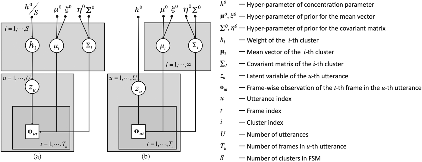
${\cal D}\lpar {\bf h}^{0}\rpar $ denotes the Dirichlet distribution with a hyper parameter h0 = {h 0/S,…,h 0/S} and ![]() ${\cal NG}$ (μd0, ξ0, η0, σdd0) denotes the Gaussian–Gamma distribution with hyper parameters μd0, ξ0, η0, and σdd0. Note that these hyper-parameters do not depend on each clusterFootnote 2. The graphical model for this model is shown in Fig. 1(a). Using these prior distributions, we can derive the joint distribution for the complete data case.
${\cal NG}$ (μd0, ξ0, η0, σdd0) denotes the Gaussian–Gamma distribution with hyper parameters μd0, ξ0, η0, and σdd0. Note that these hyper-parameters do not depend on each clusterFootnote 2. The graphical model for this model is shown in Fig. 1(a). Using these prior distributions, we can derive the joint distribution for the complete data case.

Fig. 1. Graphical models of utterance-oriented mixture models for (a) finite and (b) infinite speakers.
1) Marginalized likelihood for the complete data case
For the complete data case, the posterior probabilities of the latent variables, P(Z|O), return 0 or 1 because all assignments of utterances to speaker clusters are available. Then, the sufficient statistics of this model can be described as follows:
 $$\left\{{\matrix{ n^{utt}_{i} &= \sum\nolimits_{u} \delta\lpar z_{u}\comma \; i\rpar \comma \; \hfill \cr n^{frm}_{i} &= \sum\nolimits_{u} \delta\lpar z_{u}\comma \; i\rpar T_{u}\comma \; \hfill \cr {\bf m}_{i} &= \sum\nolimits_{u} \delta\lpar z_{u}\comma \; i\rpar \sum\nolimits_{t} {\bf o}_{ut}\comma \; \hfill \cr r_{i\comma dd} &= \sum\nolimits_{u} \delta\lpar z_{u}\comma \; i\rpar \sum\nolimits_{t} \lpar o_{ut\comma d}\rpar^{2}\comma \; \hfill \cr}} \right.$$
where n iutt and n ifrm are the number of utterances and that of frames assigned to the ith cluster, respectively; mi and r i, dd are the first- and second-order sufficient statistics, respectively. Using equations (2) and (4), the likelihood for the complete data case can be expressed as follows:
Here, recalling that the speaker clustering problem aims to estimate the optimal assignment of utterances to speaker clusters, we can see that the parameter Θ need not be estimated. We can therefore marginalize this parameter out from the joint distribution described in equation (5). This marginalization allows us to optimize the model on the latent variable space. By restricting the search space of the latent variables, we can obtain a model estimation algorithm that is robust against the local optima problem.
From equations (3) and (5), the marginalized likelihood for the complete data case, integrated using the parameter Θ, can be factorized to the following two integrals:
 $$\eqalign{p\lpar {\bf O}\comma \; {\bf Z}\rpar &= \!\vint\! p\lpar {\bf O}\comma \; {\bf Z} \vert {\bf \Theta}\comma \; {\bf h}\rpar \cdot p\lpar {\bf \Theta}\comma \; {\bf h}\rpar {d}{\bf \Theta} {d}{\bf h} \cr & = \!\vint\! P\lpar {\bf Z} \vert {\bf h}\rpar p\lpar {\bf h}\rpar {d}{\bf h}\cdot\! \vint\!\! p\lpar {\bf O} \vert {\bf Z}\comma \; {\bf \Theta}\rpar p\lpar {\bf \Theta}\rpar {d}{\bf \Theta}.}$$
The first term on the right-hand side of equation (6) is described as follows:
 $$\vint P\lpar {\bf Z} \vert {\bf h}\rpar p\lpar {\bf h}\rpar {d}{\bf h} = C\lpar {\bf h}^{0}\rpar \displaystyle{{ \prod_{i} \Gamma\lpar {\tilde h}_{i}\rpar } \over { \Gamma\lpar \sum_{i} {\tilde h}_{i}\rpar }}\comma \;$$
where C(h0) denotes the normalization term that is independent of n utti. The second term on the right-hand side of equation (6) is described as follows:
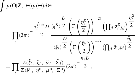 $$\eqalign{& \vint p\lpar {\bf O} \vert {\bf Z}\comma \; {\bf \Theta}\rpar p\lpar {\bf \Theta}\rpar {d}{\bf \Theta} \cr & \quad = \prod_{i} \lpar 2\pi\rpar ^{-\displaystyle{{n^{ frm}_{i}D} \over{2}}} \displaystyle{{\lpar \xi^{0}\rpar ^{\displaystyle{{D}\over{2}}} \left(\Gamma\left(\displaystyle{{\eta_{i}^{0}}\over{2}}\right)\right)^{-D} \left(\prod_{d}\sigma_{i\comma dd}^{0}\right)^{\displaystyle{{\eta_{i}^{0}} \over {2}}} } \over { \lpar {\tilde \xi}_{i}\rpar ^{\displaystyle{{D}\over{2}}} \left(\Gamma\left(\displaystyle{{{\tilde \eta}_{i}}\over{2}}\right)\right)^{-D} \left(\prod_{d}{\tilde \sigma}_{i\comma dd}\right)^{\displaystyle{{{\tilde \eta}_{i}} \over {2}}}}} \cr & \quad = \prod_{i} \displaystyle{{Z\lpar {\tilde \xi}_{i}\comma \; {\tilde \eta}_{i}\comma \; {\bf{\tilde \mu}}_{i}\comma \; {\bf{\tilde \Sigma}}_{i}\rpar } \over {Z\lpar \xi^{0}\comma \; \eta^{0}\comma \; {\bf \mu}^{0}\comma \; {\bf \Sigma}^{0}\rpar }} \lpar 2\pi\rpar ^{-\displaystyle{{n_{i}D} \over {2}}}\comma \; }$$
where ![]() ${\bf{\tilde \Theta}}\triangleq \lcub {\tilde h}_{i}\comma \; {\tilde \eta}_{i\comma dd}\comma \; {\tilde \xi}_{i\comma dd}\comma \; {\bf{\tilde \mu}}_{i}\comma \; {\tilde \sigma}_{i\comma dd} \rcub $ denotes the hyper-parameter of the posterior distribution for Θ, which is described as follows:
${\bf{\tilde \Theta}}\triangleq \lcub {\tilde h}_{i}\comma \; {\tilde \eta}_{i\comma dd}\comma \; {\tilde \xi}_{i\comma dd}\comma \; {\bf{\tilde \mu}}_{i}\comma \; {\tilde \sigma}_{i\comma dd} \rcub $ denotes the hyper-parameter of the posterior distribution for Θ, which is described as follows:
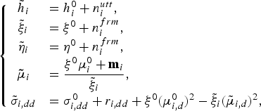 $$\left\{{\matrix{{\tilde h}_{i} &= h_{i}^{0} + n^{utt}_{i}\comma \; \hfill \cr {\tilde \xi}_{i} &= \xi^{0} + n^{frm}_{i}\comma \; \hfill \cr {\tilde \eta}_{i} &= \eta^{0} + n^{frm}_{i}\comma \; \hfill \cr {\bf{\tilde \mu}}_{i} &= \displaystyle{{\xi^{0}{\bf \mu}_{i}^{0} + {\bf m}_{i}} \over {{\tilde \xi}_{i}}}\comma \; \hfill \cr {\tilde \sigma}_{i\comma dd} & = \sigma_{i\comma dd}^{0} + r_{i\comma dd} + \xi^{0}\lpar \mu_{i\comma d}^{0}\rpar^2 - {\tilde \xi}_{i}\lpar {\tilde \mu}_{i\comma d}\rpar^2\comma \; }}\right.$$
where we have used equation (4).
2) MCMC-based posterior estimation
We again emphasize that the speaker clustering problem is reduced to the estimation of the latent variables Z, which maximize the posterior distribution P(Z|O). We can then derive the posterior distribution for the latent variables as p(Z|O) ∝ p(O,Z). The evaluation of all combinations of these latent variables in p(Z|O), however, is obviously infeasible if the number of utterances (i.e. the number of latent variables) is large. Instead, we use collapsed Gibbs sampling [Reference Liu11] to obtain the optimal value of Z directly from its posterior distribution P(Z |O).
In each step of the collapsed Gibbs sampling process, the value of one of the latent variables (e.g. z u) is replaced with a value generated from the distribution of that variable given the values of the remaining latent variables (i.e. ![]() ${\bf Z}_{\backslash u}^{\ast} = \lcub z_{u^{\prime}} \vert u^{\prime} \neq u\rcub $). In this case, the latent variables are sampled from the conditional posterior distribution as follows:
${\bf Z}_{\backslash u}^{\ast} = \lcub z_{u^{\prime}} \vert u^{\prime} \neq u\rcub $). In this case, the latent variables are sampled from the conditional posterior distribution as follows:
 $$\eqalign{& P\lpar z_{u}=i^{\prime} \vert {\bf O}\comma \; {\bf Z}^{\ast}_{\backslash u}\rpar \cr & \quad \propto P\lpar z_{u} = i^{\prime} \vert {\bf Z}^{\ast}_{\backslash u}\rpar \cdot p\lpar {\bf O}_{u} \vert {\bf O}_{\backslash u}\comma \; {\bf Z}_{\backslash u}^{\ast}\comma \; z_{u} = i^{\prime} \rpar \cr & \quad = \displaystyle{{ P\lpar {\bf Z}_{\backslash u}^{\ast}\comma \; z_{u}=i^{\prime}\rpar } \over { P\lpar {\bf Z}_{\backslash u}^{\ast}\rpar }} \cdot \displaystyle{{ p\lpar {\bf O}_{u}\comma \; {\bf O}_{\backslash u} \vert {\bf Z}_{\backslash u}^{\ast}\comma \; z_{u} = i^{\prime}\rpar } \over { p\lpar {\bf O}_{\backslash u} \vert {\bf Z}_{\backslash u}^{\ast}\rpar }}.}$$
 Note that the hyper-parameters of prior distributions, ![]() $\lcub {\bf h}^{0}\comma \; {\bf \Theta}^{0}\rcub $, are omitted in equation (10). From equation (7), the first term on the right-hand side of equation (10) can be described as follows:
$\lcub {\bf h}^{0}\comma \; {\bf \Theta}^{0}\rcub $, are omitted in equation (10). From equation (7), the first term on the right-hand side of equation (10) can be described as follows:
 $$\displaystyle{{P\lpar {\bf Z}_{\backslash u}^{\ast}\comma \; z_{u} = i^{\prime}\rpar }\over {P\lpar {\bf Z}_{\backslash u}^{\ast}\rpar }} = \displaystyle{{\displaystyle{{h^{0}}\over{S}}+n_{i^{\prime}}} \over {U-1+h^{0}.}}$$
From equation (8), the second term on the right-hand side of equation (10) is described as follows:
 $$\displaystyle{{ p\lpar {\bf O} \vert {\bf Z}_{\backslash u}^{\ast}\comma \; z_{u} = i^{\prime}\rpar } \over { p\lpar {\bf O}_{\backslash u} \vert {\bf Z}_{\backslash u}^{\ast}\rpar }} \propto \exp\lpar g_{i^{\prime}}\lpar {\bf{\tilde \Theta}}_{i^{\prime}}\rpar -g_{i^{\prime}}\lpar {\bf{\tilde \Theta}}_{i^{\prime}\backslash u}\rpar \rpar \comma \;$$
where
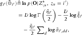 $$\eqalign{ {g_{i^{\prime}}}\lpar {{\bf {\tilde \Theta}}_{i^{\prime}}}\rpar & \triangleq \ln p \lpar {\bf O} \vert Z_{\backslash u}^{\ast}\comma \; {z_u} = i^{\prime}\rpar \cr & = D \log \Gamma \left({\displaystyle{{{{\tilde \eta }_{i^{\prime}}}} \over 2}}\right)- \displaystyle{D \over 2}\log {{\tilde \xi }_{i^{\prime}}} \cr & \quad - \displaystyle{{{{\tilde \eta }_{i^{\prime}}}} \over 2}\sum\nolimits_d {\log {{\tilde \sigma }_{i^{\prime}\comma dd}}\comma \; } }$$
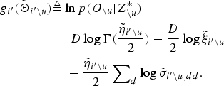 $$\eqalign{ {g_{i^{\prime}}}\lpar {{\tilde \Theta }_{i^{\prime}\backslash u}}\rpar & \triangleq \ln p \lpar {O_{\backslash u}} \vert Z_{\backslash u}^{\ast}\rpar \cr & = D\log \Gamma \lpar \displaystyle{{{{\tilde \eta }_{i^{\prime}\backslash u}}} \over 2}\rpar - \displaystyle{D \over 2}\log {{\tilde \xi }_{i^{\prime}\backslash u}} \cr & \quad - \displaystyle{{{{\tilde \eta }_{i^{\prime}\backslash u}}} \over 2}\sum\nolimits_d {\log {{\tilde \sigma }_{i^{\prime}\backslash u\comma dd}}.} }$$
 ![]() ${\bf{\tilde \Theta}}_{i^{\prime}\backslash u}$ in equation (14) denotes the hyper-parameter of the posterior distribution for Θ after removing uth utterance, which is described as follows:
${\bf{\tilde \Theta}}_{i^{\prime}\backslash u}$ in equation (14) denotes the hyper-parameter of the posterior distribution for Θ after removing uth utterance, which is described as follows:
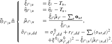 $${\bf{\tilde \Theta}}_{i^{\prime}\backslash u}\triangleq \left\{{\matrix{ {\tilde \xi}_{i^{\prime}\backslash u} & = {\tilde \xi}_{i} - T_u\comma \; \hfill \cr {\tilde \eta}_{i^{\prime}\backslash u} & = {\tilde \eta}_{i} - T_u\comma \; \hfill \cr {\bf{\tilde \mu}}_{i^{\prime}\backslash u} &= \displaystyle{{ {\tilde \xi}_{i^{\prime}} {\bf{\tilde \mu}}_{i^{\prime}} - \sum_{t}{\bf o}_{ut} } \over {{\tilde \xi}_{i^{\prime}\backslash u}}}\comma \; \hfill \cr {\tilde \sigma}_{i^{\prime}\backslash u\comma dd} & = \sigma_{i^{\prime}\comma dd}^{0} + r_{i^{\prime}\comma dd} - \sum_{t}\lpar o_{ut\comma d}\rpar^2 \cr & \quad+ \xi^{0}\lpar \mu_{i^{\prime}\comma d}^{0}\rpar^2 - {\tilde \xi}_{i^{\prime}\backslash u}\lpar {\tilde \mu}_{i^{\prime}\backslash u\comma d}\rpar^2.}}\right.$$
The optimal values of Z (i.e. the optimal assignments of utterances to clusters) can be obtained from its posterior distribution P(Z|O) by iterating to sample z u from its conditional posterior distribution in equation (10) until convergence.
III. UTTERANCE-ORIENTED MIXTURE MODEL FOR INFINITE SPEAKERS
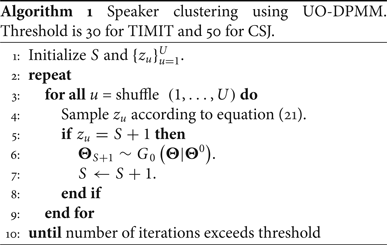
In this section, we attempt to extend the utterance-oriented mixture model for finite speakers in order to deal with infinite speakers. For this purpose, we introduce Dirichlet process as the prior distribution of mixture weights. The derived model (i.e. the UO-DPMM) is a type of Dirichlet process mixture model (DPMM) [Reference Ferguson5], but it differs from the original DPMM in that the generative unit is not a frame but rather an utterance. In the present study, UO-DPMM was built using Chinese restaurant process (CRP) [Reference Aldous12], which can avoid local solutions because of its sampling-based implementation. Furthermore, we can easily integrate CRP with other sophisticated methods, such as simulated annealing. The graphical model of the utterance-oriented mixture model for infinite speakers is shown in Fig. 1(b). Table 1 provides a pseudo code of this method.
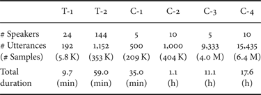
Table 1. Details of test set. # speakers, # utterances, # samples, and total duration denote the number of speakers, number of utterances, number of frame-wise observations, and total duration.

CRP is found by taking the limit of S (i.e. S → ∞) in equation (10). Note that there are at most U (<S) speaker clusters to which at least one utterance is assigned. In the case of S being infinite, most clusters should be empty. In this case, we can separately compute equation (11) for the case where the uth utterance is assigned to a cluster with more than one utterance (i.e. n i′ > 0) and the case where the uth utterance is assigned to a new cluster with no utterance (i.e. n i′ = 0).
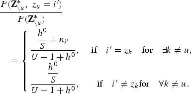 $$\eqalign{& \displaystyle{{P\lpar {\bf Z}_{\backslash u}^{\ast}\comma \; z_{u}=i^{\prime}\rpar } \over {P\lpar {\bf Z}_{\backslash u}^{\ast}\rpar }} \cr & \quad = \left\{{\matrix{\displaystyle{{\displaystyle{{h^{0}} \over{S}} +n_{i^{\prime}}} \over {U-1+h^{0}}}\comma \; & \hbox{if} \quad i^{\prime} = z_{k} \quad \hbox{for} \quad \exists k \neq u\comma \; \cr \displaystyle{{\displaystyle{{h^{0}} \over {S}}} \over {U-1+h^{0}}}\comma \; & \hbox{if} \quad i^{\prime} \neq z_{k} \hbox{for} \quad \forall k \neq u. \cr}}\right.}$$
By taking the limit of S → ∞, the number of utterances U satisfies U≪S and thus we can assume that there are S empty clusters. Therefore, by combining the empty clusters, equation (16) is described as follows:
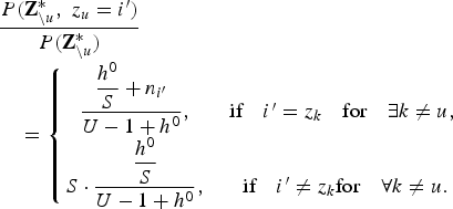 $$\eqalign{& \displaystyle{{P\lpar {\bf Z}_{\backslash u}^{\ast}\comma \; z_{u}=i^{\prime}\rpar } \over {P\lpar {\bf Z}_{\backslash u}^{\ast}\rpar }} \cr & \quad = \left\{{\matrix{\displaystyle{{\displaystyle{{h^{0}} \over {S}} +n_{i^{\prime}}} \over {U-1+h^{0}}}\comma \; & \hbox{if}\quad i^{\prime}=z_{k}\quad \hbox{for}\quad \exists k \neq u\comma \; \cr S \cdot \displaystyle{{\displaystyle{{h^{0}} \over {S}}}\over {U-1+h^{0}}}\comma \; & \hbox{if}\quad i^{\prime} \neq z_{k} \hbox{for} \quad \forall k \neq u. \cr}}\right. }$$
Taking the limit of S → ∞ in equation (17) allows us to derive the following equation:
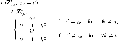 $$\eqalign{& \displaystyle{{P\lpar {\bf Z}_{\backslash u}^{\ast}\comma \; z_{u}=i^{\prime}\rpar } \over {P\lpar {\bf Z}_{\backslash u}^{\ast}\rpar }} \cr & \quad = \left\{{\matrix{\displaystyle{{n_{i^{\prime}}} \over {U-1+h^{0}}}\comma \; & \hbox{if} \quad i^{\prime} = z_{k} \quad \hbox{for} \quad \exists k \neq u\comma \; \cr \displaystyle{{h^{0}} \over {U-1+h^{0}}}\comma \; & \hbox{if} \quad i^{\prime} \neq z_{k} \quad \hbox{for} \quad \forall k \neq u.\cr}}\right.}$$
From equation (8), we can also separately compute the second term on the right-hand side of equation (10) as follows:
 $$\displaystyle{{p\lpar {\bf O}\comma \; {\bf Z}_{\backslash u}^{\ast}\comma \; z_u = i^{\prime}\rpar } \over { p\lpar {\bf O}_{\backslash u}\comma \; {\bf Z}_{\backslash u}^{\ast}\rpar }} = \left\{{\matrix{\exp\lpar g_{i^{\prime}}\lpar {\bf{\tilde \Theta}}_{i^{\prime}}\rpar - g_{i^{\prime}}\lpar {\bf{\tilde \Theta}}_{i^{\prime}\backslash u}\rpar \rpar \comma \; \cr \quad \hbox{if}\quad z_k = i^{\prime}\quad \hbox{for}\quad \exists k \neq u \cr \exp\lpar g_{new}\lpar {\bf{\tilde \Theta}}_{new}\rpar - g_{new}\lpar {\bf \Theta}_{0}\rpar \rpar \cr \quad \hbox{if}\quad z_{k} \neq i^{\prime}\quad \hbox{for}\quad \forall k \neq u\comma \; }}\right.$$
where ![]() $g_{new}\lpar {\bf{\tilde \Theta}}_{new}\rpar $ and
$g_{new}\lpar {\bf{\tilde \Theta}}_{new}\rpar $ and ![]() $g_{new}\lpar {\bf \Theta}_{0}\rpar $ denote the logarithmic likelihood for Ou to the new cluster, and the prior likelihood of the parameter itself, respectively.
$g_{new}\lpar {\bf \Theta}_{0}\rpar $ denote the logarithmic likelihood for Ou to the new cluster, and the prior likelihood of the parameter itself, respectively.
We can evaluate both ![]() $g_{new}\lpar {\bf{\tilde \Theta}}_{new}\rpar $ and
$g_{new}\lpar {\bf{\tilde \Theta}}_{new}\rpar $ and ![]() $g_{new}\lpar {\bf \Theta}_{0}\rpar $ using equation (13), noting that only the uth utterance is assigned to the new cluster for
$g_{new}\lpar {\bf \Theta}_{0}\rpar $ using equation (13), noting that only the uth utterance is assigned to the new cluster for ![]() $g_{new}\lpar {\bf{\tilde \Theta}}_{new}\rpar $ and no ones are assigned to the new cluster for
$g_{new}\lpar {\bf{\tilde \Theta}}_{new}\rpar $ and no ones are assigned to the new cluster for ![]() $g_{new}\lpar {\bf \Theta}_{0}\rpar $.
$g_{new}\lpar {\bf \Theta}_{0}\rpar $.
That is, we can respectively evaluate ![]() $g_{new}\lpar {\bf \Theta}_{0}\rpar $ and
$g_{new}\lpar {\bf \Theta}_{0}\rpar $ and ![]() $g_{new}\lpar {\bf{\tilde \Theta}}_{new}\rpar $ by substituting
$g_{new}\lpar {\bf{\tilde \Theta}}_{new}\rpar $ by substituting ![]() ${\bf tilde{\Theta}}_{i^{\prime}}$ in equation (13) to Θ0 and
${\bf tilde{\Theta}}_{i^{\prime}}$ in equation (13) to Θ0 and ![]() ${\bf{\tilde \Theta}}_{new}$, which is described as follows:
${\bf{\tilde \Theta}}_{new}$, which is described as follows:
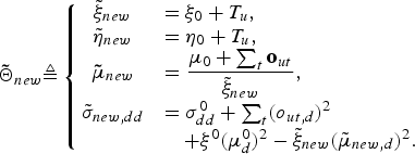 $${\bf{\tilde \Theta}}_{new} \triangleq \left\{{\matrix{{\tilde \xi}_{new} &= \xi_{0} + T_u\comma \; \hfill \cr {\tilde \eta}_{new} &= \eta_{0} + T_u\comma \; \hfill \cr {\bf{\tilde \mu}}_{new} &= \displaystyle{{{\bf \mu}_{0} + \sum_{t}{\bf o}_{ut}}\over {{\tilde \xi}_{new}}}\comma \; \hfill \cr {\tilde \sigma}_{new\comma dd} &= \sigma_{dd}^{0} + \sum_{t}\lpar o_{ut\comma d}\rpar^2 \hfill \cr & \quad + \xi^{0}\lpar \mu_{d}^{0}\rpar^2 - {\tilde \xi}_{new}\lpar {\tilde \mu}_{{ new}\comma d}\rpar^2.}} \right.$$
From equations (18) and (19), the posterior probability of the latent variables can be finally described as follows:
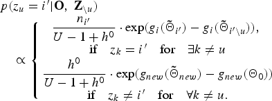 $$\eqalign{ & p\lpar z_{u}=i^{\prime} \vert {\bf O}\comma \; {\bf Z}_{\backslash u}\rpar \cr & \quad \propto \left\{{\matrix {\displaystyle{{n_{i^{\prime}}} \over {U-1+h^{0}}}\cdot \exp \lpar {g_{i}\lpar {\bf{\tilde \Theta}}_{i^{\prime}}\rpar - g_{i}\lpar {\bf{\tilde \Theta}}_{i^{\prime}\backslash u}\rpar }\rpar \comma \; \cr \hbox{if}\quad z_k = i^{\prime}\quad \hbox{for}\quad \exists k \neq u \cr \displaystyle{{h^{0}} \over {U-1+h^{0}}} \cdot \exp\lpar g_{new}\lpar {\bf{\tilde \Theta}}_{new}\rpar - g_{new}\lpar {\bf \Theta}_{0}\rpar \rpar \cr \hbox{if} \quad z_{k} \neq i^{\prime}\quad \hbox{for}\quad \forall k \neq u. \cr}}\right.}$$
We iteratively reassign each utterance to one of the existing clusters or the new cluster in proportion to equation (21) until the value of the samples converges. As shown in equation (21), the hyper-parameter h 0 determines how frequently each utterance is reassigned to the new cluster. The estimated number of speaker clusters, therefore, depends on the value of h 0. In the next section, we demonstrate that this parameter can be tuned using a development set.
IV. SPEAKER CLUSTERING EXPERIMENTS
We carried out the speaker clustering experiments using the TIMIT [Reference Garofolo, Lamel, Fisher, Fiscus, Pallett and Dahlgren13] and Corpus of Spontaneous Japanese (CSJ) [Reference Maekawa, Koiso, Furui and Isahara14] databases. We compared UO-DPMM described in Section III with existing HAC based on the Bayesian information criterion (HAC-BIC) [Reference Chen and Gopalakrishnan1] in speaker clustering with estimation of the number of speakers.
HAC-BIC is similar to UO-DPMM in terms of the model structure, i.e. both methods assume that each speaker can be represented by a single Gaussian and estimate the number of clusters using model complexity. Here, the aim of the present study is to verify if the model-based speaker clustering approach can be extended so as to estimate the number of speakers by incorporating the non-parametric Bayesian techniques in the utterance-oriented speaker mixture model. We therefore are determined to focus on comparing UO-DPMM and HAC-BIC to make this experiment comparable.
Algorithm 1 Speaker clustering using UO-DPMM. Threshold is 30 for TIMIT and 50 for CSJ.

A) Speech data
We performed the speaker clustering experiments using six evaluation sets obtained from the TIMIT and CSJ databases. We used two evaluation sets in TIMIT. T-1 was the “core test set”, which included 192 utterances spoken by 24 speakers. T-2 was the “complete test set”, which excluded the core test set in the TIMIT database and included 1152 utterances spoken by 144 speakers. T-1 and T-2 are balanced data, in which each speaker spoke the same number of utterances. The remaining four evaluation sets were obtained from lectures in CSJ as follows. First, all lectures were divided into utterance units based on the segments of silence in their transcriptions that were longer than 500 ms; 5 and 10 speakers were then randomly selected and their 100 utterances were selected for C-1 and C-2. Each utterance was between 2 and 10 s long. Next, we selected another 5 and 10 speakers and all their utterances for C-3 and C-4. C-3 and C-4 are “unbalanced” and large-scale data (they include approximately 4 and 6 million samples, respectively). Table 1 lists the number of speakers and utterances in the evaluation sets used. Speech data were sampled at 16 kHz and quantized into 16-bit data.
We used 12-dimensional mel-frequency cepstrum coefficients (MFCCs) as the feature parameters. The frame length and shift were 25 and 10 ms, respectively.
B) Measurement
We used the average cluster purity (ACP), the average speaker purity (ASP), and their geometric mean value (K) for the evaluation criteria in speaker clustering [Reference Solomonoff, Mielke, Schmidt and Gish15]. The correct speaker labels for utterances were manually annotated. Let S T be the correct number of speakers, S the estimated number of speakers, n ij the estimated number of utterances assigned to speaker cluster i in all utterances of speaker j, n j the estimated number of utterances of speaker j, n i the estimated number of utterances assigned to speaker cluster i, and U the total number of utterances. Cluster purity p i, speaker purity q j, and the K value are then calculated as follows:
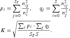 $$\eqalign{p_{i} & =\sum_{j=0}^{S_{T}} \displaystyle{{n_{ij}^{2}} \over {n_{i}^{2}}}\comma \; \quad q_{j}=\sum_{i=0}^{S} \displaystyle{{n_{ij}^{2}} \over {n_{j}^{2}}}\comma \; \cr K &= \sqrt{\displaystyle{{\sum_{i}p_{i} \cdot \sum_{j}q_{j}} \over {S_{T}S}}}.}$$
We additionally calculated the speaker diarization error rate (DER) [Reference Fiscus, Ajot and Garofolo16] in the experiments for CSJ. The DER is the ratio of incorrectly attributed speech time, which is calculated as follows:
where U fa denotes the total length of utterances not aligned with the speaker labels in the case where S T > S (i.e. false alarm utterances), namely the speech time of utterances assigned to improper speakers in the case that the estimated number of speakers is larger than the true number of speakers. U error denotes the total length of utterances aligned with the wrong speaker labels and U ref denotes the total length of all utterances in a test set. The clustering result and speaker labels concurred in order to minimize DER.
The number of iterations was set to 50 for TIMIT and 30 for CSJ. We considered the first 49 and 29 iterations for TIMIT and CSJ as the burn-in periods, respectively, leading the K values obtained from these periods to be rejected. The K value from the remaining one iteration was then measured. We carried out the same experiment 50 times but using different seeds to generate random numbers and then measured the average of their K values.
C) Experimental setup
The hyper-parameters in equation (3) were set as follows: h 0 = 1, ξ0 = 1, and η0 = 1. μi0 and Σi0 were computed as the mean and covariance of all data used in the database. In this experiment, we first estimated the optimal number of clusters as well as the optimal assignments of utterances to clusters. Next, we carried out the speaker clustering experiments using the TIMIT and CSJ databases. We then cross-validated for each pair of {T-1, T-2}, {C-1, C-2}, and {C-3, C-4} to decide the penalty parameter in the BIC-based method and the hyper-parameter h 0 in UO-DPMM.
D) Experimental results
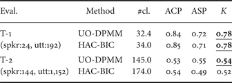
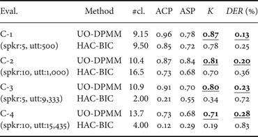
Table 2 lists the speaker clustering results for TIMIT. These results show that UO-DPMM outperformed BIC-HAC in terms of estimating the number of speakers for both T-1 and T-2. UO-DPMM also outperformed BIC-HAC in terms of the K value for T-2. Table 3 shows the speaker clustering results for CSJ. UO-DPMM outperformed BIC-HAC for all evaluation sets. Specifically, BIC-HAC performed considerably worse for C-3 and C-4. These results indicate that UO-DPMM can be robustly estimated for the unbalanced and large-scale data, while BIC-HAC significantly diminishes the clustering accuracy for these data.
Table 2. Speaker clustering results for TIMIT. #cl. denotes the number of clusters estimated.

Table 3. Speaker clustering results for CSJ.#cl. denotes the number of clusters estimated.

Next, we discuss the convergence of the sampling procedure in UO-DPMM. For that purpose, experiments were conducted with the same dataset but different seeds of a pseudo-random number generator.
Figure 2 shows the K values obtained from UO-DPMM. The eight lines in each figure show the respective results from the eight trials using the different seeds. This figure shows that all samples from all trials converge to the unique distributions. This result indicates that the proposed method is robust against the local optima problem depending on the initial states.

Fig. 2. K values obtained from proposed method for (a) T-1, (b) T-2, (c) C-1, (d) C-2, (e) C-3, and (f) C-4. Eight lines in each figure show results of eight trials using different seeds.
Finally, we discuss computational costs. In the experiment for C-4, UO-DPMM took 11.8 s per iteration and 588 s for 50 iterations on average when Intel Xeon 3.00 GHz was used. UO-DPMM required comparatively less computation time because of its fast convergence, although sampling-based methods generally require many iterations until the value of the samples converges. Figure 2 shows that all samples converge to the unique distributions within 30 iterations for all datasets. The advantage of UO-DPMM is yielded using utterance-oriented sampling. The general Gibbs sampler induces the slow convergence speed due to its sampling procedure in which only one sample is reassigned in each iteration. In contrast, the utterance-oriented sampling simultaneously reassigns a set of frames in each iteration.
V. DISCUSSION
We employed non-parametric Bayesian techniques to make it possible to estimate the number of speakers in the model-based speaker clustering system. A recently proposed sticky hierarchical Dirichlet process hidden Markov model (HDP-HMM) [Reference Fox, Sudderth, Jordan and Willsky17] is another approach to incorporate a non-parametric Bayesian manner in model-based speaker clustering. Here, we discuss the difference between UO-DPMM and HDP-HMM.
The most obvious difference is a generative unit. The unit is an utterance in UO-DPMM but a frame in HDP-HMM. This difference affects the definition of latent variables and the inference method of those variables. In UO-DPMM, the latent variable is defined for each utterance, which is composed of a set of frames, and sampled from the posterior distribution conditioned on the other utterances. In HDP-HMM, on the other hand, the latent variable is defined for each frame and sampled from the posterior distribution conditioned on the other frames. UO-DPMM, therefore, converges much faster than HDP-HMM when the boundaries of speech are given. In fact, HDP-HMM needs over 10 000 iterations of Gibbs sampling and is hard to apply on the large-scale data that we deal with in the present study.
In this paper, we introduced MCMC-based approach to estimate the model structure of UO-DPMM. Frame-wise observation approach for DPMM is addressed in previous researches [Reference Valente7,Reference Torbati, Picone and Sobel18]. In these methods, however, MCMC-based approach is not applicable because sampling of frame-wise hidden variables requires impractically heavy computational cost. In order to avoid this computation, these methods introduce the deterministic approach based on stick-breaking process [Reference Valente7] and variational Bayesian method [Reference Torbati, Picone and Sobel18]. These methods however often suffer from local solutions and overlearning problems. The proposed UO-DPMM, on the other hand, realizes MCMC-based approach by introducing the utterance-oriented assumption.
VI. CONCLUSION AND FUTURE WORK
A non-parametric Bayesian speaker modeling based on UO-DPMM was proposed to make it possible to estimate the number of speakers in model-based speaker clustering. The experimental comparison demonstrated that the proposed method was successfully applied to speaker clustering on practically large-scale data and outperformed the existing HAC method.
The present study assumed that each speaker is distributed in accordance with a Gaussian. The speaker distribution can be represented by a GMM instead of a single Gaussian, and each utterance can be assumed to be generated from a mixture of these GMMs (MoGMMs). GMM-based speaker distributions have been applied to the HAC-based speaker clustering, i.e. HAC-GMM. We have also already developed utterance-oriented speaker modeling with MoGMMs for the finite speakers [Reference Watanabe, Mochihashi, Hori and Nakamura2,Reference Tawara, Ogawa, Watanabe and Kobayashi3]. In future, we aim to derive an effective Gibbs sampling algorithm to incorporate the GMM-based speaker distributions in UO-DPMM and compare it with HAC-GMM.
ACKNOWLEDGEMENTS
This work was supported in part by Grants for Excellent Graduate Schools, MEXT, Japan.
APPENDIX
This appendix derives the joint posterior distribution p(O,Z) described in equation (5) along with the Dirichlet and Gaussian–Gamma conjugate priors.
Priors:
The Dirichlet distribution is written as
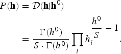 $$\eqalign{P\lpar {\bf h}\rpar &= {\cal D}\lpar {\bf h} \vert {\bf h}^{0}\rpar \cr & = \displaystyle{{\Gamma\lpar h^{0}\rpar } \over {S \cdot \Gamma\lpar h^{0}\rpar }} \prod_{i} h_{i}^{\displaystyle{{h^{0}} \over {S}}-1}.}$$
The Gaussian–Gamma distributions for the parameter of the ith cluster are written as
 $$\eqalign{p\lpar {\bf \Theta}_{i}\rpar & = p\lpar {\bf \mu}_{i}\comma \; {\bf \Sigma}_{i} \vert \xi^{0}\comma \; \eta^{0}\comma \; {\bf \mu}^{0}\comma \; {\bf \Sigma}^{0} \rpar \cr & = \prod_{i} {\cal N} \lpar {\bf \mu}_{i} \vert {\bf \mu}^{0}\comma \; \lpar \xi^{0}\rpar ^{-1}{\bf \Sigma}_{i} \rpar \prod_{d} {\cal G} \lpar \sigma_{dd} \vert \eta^{0}\comma \; \sigma_{dd}^{0}\rpar \cr & = \prod_{i}\prod_{d} \displaystyle{{\xi^{0}} \over{\lpar 2\pi\rpar ^{1/2} \lpar \sigma_{i\comma dd}\rpar ^{1/2}}} \exp \!\left\{-\displaystyle{{\xi^{0}\lpar \mu_{i\comma d}-\mu_{d}^{0}\rpar^{2}} \over {2\sigma_{i\comma dd}}} \right\}\cr & \quad \times \displaystyle{{1} \over {\Gamma\lpar \eta^{0}\rpar }} \lpar \sigma_{dd}^{0}\rpar ^{\displaystyle{{\eta^{0}} \over {2}}} \sigma_{i\comma dd}^{-\eta^{0}+1} \exp\left(-\displaystyle{{\sigma_{dd}^{0}} \over {2\sigma_{i\comma dd}}} \right)\cr & = \prod_{i} \displaystyle{{\lpar \xi^{0}\rpar ^{\displaystyle{{D} \over{2}\rsqb } \!\left(\prod_{d}\sigma_{dd}^{0}\right)^{\displaystyle{{\eta^{0}}\over{2}}}} \over {\lpar 2\pi\rpar ^{D/2} \Gamma\lpar \eta^{0}\rpar ^{\displaystyle{{D} \over {2}}}}}} \!\left(\prod_{d}\sigma_{i\comma dd}\right)^{-\eta^{0}+\displaystyle{{1} \over {2}}}\cr & \quad \times \exp\!\left\{- \sum_{d}\displaystyle{{1} \over {2\sigma_{i\comma dd}}}\!\lpar \xi^{0}\lpar \mu_{i\comma d}-\mu_{d}^{0}\rpar^{2} + \sigma_{dd}^{0} \rpar \right\}\cr & = \prod_{i} \displaystyle{{1}\over {Z\lpar \xi^{0}\comma \; \eta^{0}\comma \; {\bf \mu}^{0}}\comma \; {\bf \Sigma}^{0}\rpar } \!\left(\prod_{d}\sigma_{i\comma dd}\right)^{-\eta^{0}+\displaystyle{{1} \over {2}}}\cr & \quad \times \exp\!\left\{- \sum_{d}\displaystyle{{1} \over{2\sigma_{dd}}}\!\lpar \xi^{0}\lpar \mu_{i\comma d}-\mu_{d}^{0}\rpar^{2} + \sigma_{dd}^{0} \rpar \right\}\comma \; }$$
where
 $$Z\lpar \xi^{0}\comma \; \eta^{0}\comma \; {\bf \mu}^{0}\comma \; {\bf \Sigma}^{0}\rpar = { \lpar 2\pi\rpar ^{D\over2}\Gamma\lpar \eta^{0}\rpar ^{D} \over \lpar \xi^{0}\rpar ^{D\over2} \left(\prod_{d}\sigma_{dd}^{0}\right)^{\eta^{0}\over{2}}}.$$
Joint distribution:
We derive the joint distribution for ![]() $\lcub {\bf O}\comma \; {\bf \Theta}\rcub $ by conditioning on the latent variable
$\lcub {\bf O}\comma \; {\bf \Theta}\rcub $ by conditioning on the latent variable ![]() ${\bf Z}$ as follows:
${\bf Z}$ as follows:
 $$\eqalign{& p\lpar {\bf O}\comma \; {\bf \Theta} \vert {\bf Z}\rpar \cr & \quad= p\lpar {\bf O} \vert {\bf Z}\comma \; {\bf \Theta}\rpar p\lpar {\bf \Theta}\rpar \cr & \quad = \prod_{u\comma t} p\lpar {\bf o}_{ut}\vert {\bf \mu}_{z_{u}}\comma \; {\bf \Sigma}_{z_{u}}\rpar \prod_{i} p\lpar {\bf \mu}_{i}\comma \; {\bf \Sigma}_{i} \vert \xi^{0}\comma \; \eta^{0}\comma \; {\bf \mu}^{0}\comma \; {\bf \Sigma}^{0}\rpar \cr & \quad= \prod_{u\comma t} \left\{{\lpar 2\pi\rpar^{D\over2}\over {Z\lpar \xi^{0}\comma \; \eta^{0}\comma \; {\bf \mu}^{0}\comma \; {\bf \Sigma}^{0}\rpar }} \left(\prod_{d}\sigma_{z_{t}\comma dd}\right)^{-{1\over2}} \right\}\cr & \quad \quad\times \exp\left[- \sum_{u}\sum_{t}\sum_{d} \left\{{\lpar o_{ut\comma d} - \mu_{z_{t}\comma d}\rpar^{2}}\over {2\sigma_{z_{t}\comma dd}} \right\}\right]\cr & \quad \quad\times \exp\left[- \sum_{i}\sum_{d} {1\over 2\sigma_{i\comma dd}} \lcub \xi^{0}\lpar \mu_{i\comma d}-\mu_{d}^{0}\rpar^{2} + \sigma_{dd}^{0} \rcub \right]\cr & \quad= \prod_{i} \left\{{{\lpar 2\pi\rpar^{{n_{i}^{frm}D}{2}}}\over {Z\lpar \xi^{0}\comma \; \eta^{0}\comma \; {\bf \mu}^{0}\comma \; {\bf \Sigma}^{0}\rpar }} \left(\prod_{d}\sigma_{i\comma dd}\right)^{-{n_{i}^{frm}}\over{2}} \right\}\cr & \quad \quad \times \exp\left[- \sum_{i}\sum_{d} {{1}\over{2\sigma_{i\comma dd}}} \lcub {\tilde \xi}_{i} \lpar \mu_{i\comma d} - {\tilde \mu}_{i\comma d} \rpar^{2} + {\tilde \sigma}_{i\comma dd} \rcub \right]\cr & \quad= \prod_{i} {\lpar 2\pi\rpar ^{{n_{i}^{frm}D}\over{2}} Z\lpar {\tilde \xi}_{i}\comma \; {\tilde \eta}_{i}\comma \; {\bf{\tilde \mu}}_{i}\comma \; {\bf{\tilde \Sigma}}_{i}\rpar \over Z\lpar \xi^{0}\comma \; \eta^{0}\comma \; {\bf \mu}^{0}\comma \; {\bf \Sigma}^{0}\rpar }\cr & \quad \quad \times {\cal N} \lpar {{\bf{\tilde \mu}}}_{i}\comma \; {\tilde \xi}_{i}^{-1} {{\bf \Sigma}}_{i} \rpar \prod_{d} {\cal G} \lpar {\tilde \eta}_{i}\comma \; {\tilde \sigma}_{i\comma dd} \rpar .}$$
Marginalized distribution:
We derive the likelihood for the complete data case, ![]() $p\lpar {\bf O}\comma \; {\bf Z}\rpar $, by marginalizing the joint distribution
$p\lpar {\bf O}\comma \; {\bf Z}\rpar $, by marginalizing the joint distribution ![]() $p\lpar {\bf O}\comma \; {\bf Z}\comma \; \break {\bf \Theta}\comma \; {\bf h}\rpar = p\lpar {\bf O}\comma \; {\bf \Theta} \vert {\bf Z}\rpar p\lpar {\bf Z}\comma \; {\bf h}\rpar $ with respect to the hyper-parameters
$p\lpar {\bf O}\comma \; {\bf Z}\comma \; \break {\bf \Theta}\comma \; {\bf h}\rpar = p\lpar {\bf O}\comma \; {\bf \Theta} \vert {\bf Z}\rpar p\lpar {\bf Z}\comma \; {\bf h}\rpar $ with respect to the hyper-parameters ![]() $\lcub {\bf h}\comma \; {\bf \Theta}\rcub $.
$\lcub {\bf h}\comma \; {\bf \Theta}\rcub $.
First, we derive the likelihood ![]() $P\lpar {\bf Z}\rpar $ by marginalizing
$P\lpar {\bf Z}\rpar $ by marginalizing ![]() $p\lpar {\bf Z}\comma \; {\bf h}\rpar $ with respect to
$p\lpar {\bf Z}\comma \; {\bf h}\rpar $ with respect to ![]() $\lcub {\bf w}_{i}\comma \; {\bf h}\comma \; {\bf \Theta}_{i}\rcub _{i}$. Assuming the independence of the utterance-level latent variables z u, this can be analytically derived as follows:
$\lcub {\bf w}_{i}\comma \; {\bf h}\comma \; {\bf \Theta}_{i}\rcub _{i}$. Assuming the independence of the utterance-level latent variables z u, this can be analytically derived as follows:
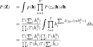 $$\eqalign{P\lpar {\bf Z}\rpar & \quad = \vint p\lpar {\bf h}\rpar \prod_{u=1}^{U} P\lpar z_{u} \vert {\bf h}\rpar {d}{\bf h} \cr & \quad = {\Gamma\lpar \sum_{i}h_{i}^{0}\rpar \over {\prod_{i}\Gamma\lpar h_{i}^{0}\rpar }} \vint \prod_{i=1}^{S} h_{i}^{\sum_{u}\delta\lpar z_{u}\comma i\rpar +h_{i}^{0}-1} {d}h_{i} \cr & \quad = {{\Gamma\lpar \sum_{i}h_{i}^{0}\rpar } {\prod_{i}\Gamma\lpar h_{i}^{0}\rpar } \over{\prod_{i}\Gamma\lpar {\tilde h}_{i}\rpar } {\Gamma\lpar \sum_{i}{\tilde h}_{i}\rpar }}.}$$
 Finally, we derive the likelihood ![]() $p\lpar \bf \Theta\rpar $ by marginalizing
$p\lpar \bf \Theta\rpar $ by marginalizing ![]() $p\lpar {\bf O}\comma \; {\bf \Theta}\rpar $ with respect to the model parameter
$p\lpar {\bf O}\comma \; {\bf \Theta}\rpar $ with respect to the model parameter ![]() ${\bf \Theta}$. Using equation (A.4), this can be analytically derived as follows:
${\bf \Theta}$. Using equation (A.4), this can be analytically derived as follows:
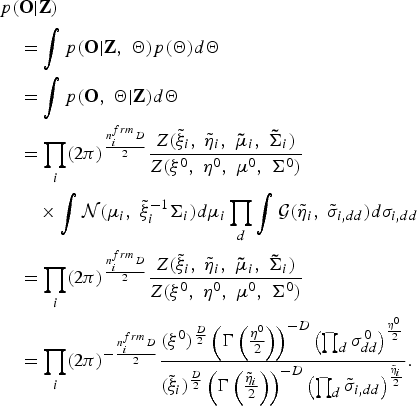 $$\eqalign{& p\lpar {\bf O} \vert {\bf Z}\rpar \cr & \quad = \vint p\lpar {\bf O} \vert {\bf Z}\comma \; {\bf \Theta}\rpar p\lpar {\bf \Theta}\rpar {d}{\bf \Theta} \cr & \quad = \vint p\lpar {\bf O}\comma \; {\bf \Theta} \vert {\bf Z}\rpar {d}{\bf \Theta} \cr & \quad = \prod_{i} \lpar 2\pi\rpar ^{n_{i}^{frm}D\over{2}} {Z\lpar {\tilde \xi}_{i}\comma \; {\tilde \eta}_{i}\comma \; {\bf{\tilde \mu}}_{i}\comma \; {\bf{\tilde \Sigma}}_{i}\rpar \over {Z\lpar \xi^{0}\comma \; \eta^{0}\comma \; {\bf \mu}^{0}\comma \; {\bf \Sigma}^{0}\rpar }} \cr & \quad \quad \times \vint {\cal N} \lpar {{\bf \mu}}_{i}\comma \; {\tilde \xi}_{i}^{-1} {{\bf \Sigma}}_{i} \rpar {d}{\bf \mu}_{i} \prod_{d} \vint {\cal G} \lpar {\tilde \eta}_{i}\comma \; {\tilde \sigma}_{i\comma dd} \rpar {d}\sigma_{i\comma dd} \cr & \quad = \prod_{i} \lpar 2\pi\rpar ^{n_{i}^{frm}D\over 2} {{Z\lpar {\tilde \xi}_{i}\comma \; {\tilde \eta}_{i}\comma \; {\bf{\tilde \mu}}_{i}\comma \; {\bf{\tilde \Sigma}}_{i}\rpar }\over {Z\lpar \xi^{0}\comma \; \eta^{0}\comma \; {\bf \mu}^{0}\comma \; {\bf \Sigma}^{0}\rpar }}\cr & \quad = \prod_{i} \lpar 2\pi\rpar ^{-{n_{i}^{frm}D\over 2}}{\lpar \xi^{0}\rpar ^{{D}\over{2}} \left(\Gamma\left({\eta^{0}\over{2}}\right)\right)^{-D} \left(\prod_{d}\sigma_{dd}^{0}\right)^{\eta^{0}\over {2}} \over \lpar {\tilde \xi}_{i}\rpar ^{{D}\over{2}} \left(\Gamma\left({\tilde \eta}_{i}\over{2}\right)\right)^{-D} \left(\prod_{d}{\tilde \sigma}_{i\comma dd}\right)^{{\tilde \eta}_{i}\over{2}}}.}$$
Using equations (A.5) and (A.6), the marginalized distribution for the complete data case can be finally described as follows:
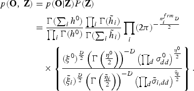 $$\eqalign{p\lpar {\bf O}\comma \; {\bf Z}\rpar &= p\lpar {\bf O} \vert {\bf Z}\rpar P\lpar {\bf Z}\rpar \cr & ={\Gamma\lpar \sum_{i}h^{0}\rpar \over{\prod_{i}\Gamma\lpar h^{0}\rpar }} {\prod_{i}\Gamma\lpar {\tilde h}_{i}\rpar \over {\Gamma\lpar \sum_{i}{\tilde h}_{i}\rpar }} \prod_{i} \lpar 2\pi\rpar ^{-{n_{i}^{frm}D\over{2}}}\cr & \quad \times\left\{{\lpar \xi^{0}\rpar^{D\over 2} \left(\Gamma\left({\eta^{0}\over 2}\right)\right)^{-D} \left(\prod_{d}\sigma_{dd}^{0}\right)^{\eta^0 \over 2} \over \lpar \tilde \xi_{i}\rpar^{D\over 2} \left(\Gamma\left({\tilde \eta_{i}\over 2}\right)\right)^{-D} \left({\prod_{d}}{\tilde \sigma}_{i\comma dd}\right)^{{\tilde \eta}_i \over 2}}\right\}.}$$
Naohiro Tawara received his B.S. and M.S. degrees from Waseda University in Tokyo, Japan in 2010 and 2012. He is currently a graduate student working towards becoming a Ph.D. candidate. He is a member of the Institute of Electronics Information and Communication Engineers and of the Acoustical Society of Japan. His research interests include speaker recognition, image processing, and machine learning.
Tetsuji Ogawa received his B.S., M.S., and Ph.D. in electrical engineering from Waseda University in Tokyo, Japan, in 2000, 2002, and 2005. He was a Research Associate from 2004 to 2007 and a Visiting Lecturer in 2007 at Waseda University. He was an Assistant Professor at Waseda Institute for Advanced Study from 2007 to 2012. He has been an Associate Professor at Waseda University and Egypt-Japan University of Science and Technology (E-JUST) since 2012. He was a Visiting Scholar in the Center for Language and Speech Processing, Johns Hopkins University, Baltimore, MD from June to September in 2012 and from June to August in 2013 and a Visiting Scholar in the Speech@FIT research group, Brno University of Technology, Brno, Czech Republic from June to July in 2014 and from May to August in 2015. His research interests include stochastic modeling for pattern recognition, speech enhancement, and speech and speaker recognition. He is a member of the Institute for of Electrical and Electronics Engineering (IEEE), Information Processing Society of Japan (IPSJ) and Acoustic Society of Japan (ASJ). He received the Awaya Prize Young Researcher Award from the ASJ in 2011 and Yamashita SIG Research Award from the IPSJ in 2013.
Shinji Watanabe is a Senior Principal Member Research Staff at Mitsubishi Electric Research Laboratories (MERL), Cambridge, MA. He received his Ph.D. from Waseda University, Tokyo, Japan, in 2006. From 2001 to 2011, he was a research scientist at NTT Communication Science Laboratories, Kyoto, Japan. From January to March in 2009, he was a visiting scholar in Georgia institute of technology, Atlanta, GA. His research interests include Bayesian machine learning and speech and spoken language processing. He has been published more than 100 papers in journals and conferences, and received several awards including the Best paper award from the IEICE in 2003. He is an Associate Editor of the IEEE Transactions on Audio Speech and Language Processing, and a member of several committees including the IEEE Signal Processing Society Speech and Language Technical Committee and the APSIPA Speech, Language, and Audio Technical Committee.
Atsushi Nakamura received the B.E., M.E., and Dr. Eng. degrees from Kyushu University, Fukuoka, Japan, in 1985, 1987, and 2001, respectively. In 1987, he joined Nippon Telegraph and Telephone Corporation (NTT), where he engaged in the research and development of network service platforms, including studies on the application of speech processing technologies to network services, at Musashino Electrical Communication Laboratories, Tokyo, Japan. From 1994 to 2000, he was with the Advanced Telecommunications Research (ATR) Institute, Kyoto, Japan, as a Senior Researcher, undertaking research on spontaneous speech recognition, the construction of spoken language databases, and the development of speech translation systems. From April, 2000 to March, 2014, he was with NTT Communication Science Laboratories, Kyoto, Japan. His research interests include the acoustic modeling of speech, speech recognition and synthesis, spoken language processing systems, speech production and perception, computational phonetics and phonology, and the application of learning theories to signal analysis, and modeling. Since April, 2014, he has been with Graduate School of Natural Sciences, Nagoya City University, Aichi, Japan. Dr. Nakamura is a senior member of the Institute of Electrical and Electronics Engineers (IEEE), served as a member of the IEEE Machine Learning for Signal Processing (MLSP) Technical Committee, and as the Chair of the IEEE Signal Processing Society Kansai Chapter. He is also a member of the Institute of Electronics, Information and Communication Engineers (IEICE) and the Acoustical Society of Japan (ASJ). He received the IEICE Paper Award in 2004, and twice received the TELECOM System Technology Award of the Telecommunications Advancement Foundation, in 2006 and 2009.
Tetsunori Kobayashi received B.E, M.E, and Dr.E. degrees from Waseda University, Japan, in 1980, 1982, and 1985, respectively. In 1985, he joined Hosei University where he served as a lecturer and then as an associate professor. In 1991, he moved to Waseda University and has been a professor there since 1997. He was a visiting researcher in MIT's Laboratory for Computer Science, Advanced Telecommunication Laboratory, and NHK's Science and Technical Research Laboratory. His research interests include the basics of speech recognition and synthesis and of image processing and applying them to conversational robots.


