


1. Introduction
The drive to develop high-speed flight vehicles leads to the need to understand the mechanisms involved in the laminar–turbulent transition process for wall-bounded compressible flows. Of particular importance are instabilities developing in the boundary layer due, for example, to surface imperfections or free-stream turbulence. Transition to turbulence in compressible flows is accompanied by increased wall temperatures and aerodynamic drag. These effects are of significance in many applications, for example, the design of thermal protection systems. Thus, how these instabilities develop and how they can be controlled (usually with the aim to delay transition to turbulence) have been the focus of an immense number of studies, experimental, numerical and theoretical, over the past several decades. Many of these investigations concerning the numerous different structures occurring in transitional (incompressible and compressible) boundary layers are reviewed by Lee & Jiang (Reference Lee and Jiang2019).
The transition process from a laminar flow to a turbulent flow in supersonic and hypersonic boundary layers is less well understood compared with incompressible flow due to additional instability modes existing, which can be dominant for large Mach numbers. Enhanced surface temperatures mean that the effect of wall cooling and the thermal properties of the surface on transition mechanisms need to be understood. For particular features associated with instabilities in hypersonic boundary layers, see the review papers of Zhong & Wang (Reference Zhong and Wang2012) for numerical studies and Fedorov (Reference Fedorov2011) for theoretical investigations. Numerical and experimental studies are complemented by asymptotic analysis, which has provided further insight into the transition process in compressible boundary-layer flows. Recent studies have shown that coherent structures can be described by asymptotic analysis of vortex–wave interaction for compressible flows. See, for example Johnstone & Hall (Reference Johnstone and Hall2021) and Zhu & Wu (Reference Zhu and Wu2022).
The current paper extends the incompressible study of Duck & Stephen (Reference Duck and Stephen2021) (hereafter referred to as DS), into the fully compressible regime. The focus of the investigation of DS was in the development of three-dimensional (3-D) disturbances with spanwise scales comparable to the boundary-layer thickness. The appropriate governing equations are the boundary-region equations (BRE), which were solved numerically, revealing unstable, unsteady solutions possible for three-dimensional disturbances, in contrast to only stable solutions existing for corresponding two-dimensional disturbances. The numerical and asymptotic analysis of DS links the solutions to two previously known unsteady two-dimensional modes, namely the Lam & Rott (Reference Lam and Rott1960) and Ackerberg & Phillips (Reference Ackerberg and Phillips1972) family of eigensolutions and the Brown & Stewartson (Reference Brown and Stewartson1973) eigenmodes. See DS for more details.
The compressible BRE have been employed to study receptivity to free-stream vortical disturbances. Ricco & Wu (Reference Ricco and Wu2007) extended the incompressible study of Leib, Wundrow & Goldstein (Reference Leib, Wundrow and Goldstein1999) to the compressible case. For low-frequency (long-wavelength) turbulent fluctuations, the far-downstream region is governed by the unsteady BRE. Growing modes were found below a critical spanwise wavenumber. This investigation has lead to many subsequent studies of flows exhibiting streamwise streaks, so-called Klebanoff modes. Klebanoff modes are formed by the entrainment of free-stream vortical disturbances into a boundary layer. They develop in the boundary layer and are characterised by having a streamwise velocity much larger than the normal and spanwise components. See for example, Marensi, Ricco & Wu (Reference Marensi, Ricco and Wu2017). A further application of these equations is in Ricco, Tran & Ye (Reference Ricco, Tran and Ye2009), who studied wall heat transfer effects on Klebanoff modes and Tollmien–Schlichting waves. Theoretical studies have been conducted which attempt to explain observed experimental results on Klebanoff modes, for example, Ricco, Luo & Wu (Reference Ricco, Luo and Wu2011) and Ricco (Reference Ricco2023).
The BRE have also been shown to be appropriate for describing Görtler vortices; streamwise streaks due to streamwise curvature. Görtler vortices occur on turbine blades and need to be considered in wind-tunnel nozzles, amongst other practical applications. Hall (Reference Hall1983) showed that a unique neutral curve did not exist as a result of the non-parallel nature of the flow. In fact, the governing parabolised Navier–Stokes equations presented in Hall (Reference Hall1983) are precisely the BRE, although this terminology was not adopted until later. Since the solutions depend on the initial conditions, receptivity, analyses are required to determine the response of the boundary layer. Wu, Zhao & Luo (Reference Wu, Zhao and Luo2011) and Xu, Zhang & Wu (Reference Xu, Zhang and Wu2017) were the first to treat streamwise streaks and Görtler vortices in the same framework in analysing the receptivity to free-stream vortical disturbances using the unsteady BRE. These studies have been extended to consider compressible effects by Viaro & Ricco (Reference Viaro and Ricco2019a,Reference Viaro and Riccob). For compressible flows the applications extend to hypersonic flow, including for example the development of hypersonic vehicles and reentry capsules. A comprehensive review on theoretical, computational and experimental studies on compressible Görtler vortices is given by Xu, Ricco & Duan (Reference Xu, Ricco and Duan2024), which identifies the role of the linear and nonlinear BRE in the theoretical frameworks. These equations were also considered in the study of Es-Sahli et al. (Reference Es-Sahli, Sescu, Zamir, Koshuriyan, Hattori and Hirota2023), where optimal conditions using suction and blowing were sought for suppressing the growth of compressible Görtler vortices. In this latter investigation the adjoint compressible BRE were solved. Overall, we see the versatility of the BRE approach and theoretical studies.
The structure of this paper is as follows. In § 2 we present the derivation of the compressible BRE, appropriate for large values of the Reynolds number, where the spanwise length scales are generally comparable to the boundary-layer thickness. In § 3 we present numerical solutions of these equations for small-amplitude, spatially developing, time-periodic, spanwise perturbations about a steady compressible boundary-layer flow. Solutions exhibiting downstream growth are presented. As in DS, a local stability analysis based upon the parabolic-flow approximation is considered in § 4. The effect of Mach number on the growth rates of unstable modes is determined for supersonic conditions. The analysis for the far-downstream limit is presented in § 5. In the first instance, unstable modes analogous to those in DS and stable Lam & Rott (Reference Lam and Rott1960) eigenmodes are considered. For the unstable non-entropy modes we find that the effect of compressibility is in some cases represented by one parameter. This allows for easy determination of the growth rates for larger spanwise wavenumbers using the corresponding incompressible results of DS. Further analysis suggests that an additional scaling of the spanwise wavenumber is appropriate (even) further downstream. Consideration of this reveals new unstable modes in the compressible case (not found in the incompressible case), described by an inviscid analysis. Comparisons of the asymptotic results with the numerical solutions are presented. Finally, the downstream development of entropy modes is considered for  $O(1)$ spanwise wavenumbers, with a local analysis based upon a parallel-flow approximation indicating that they are always stable. However, there is a slight caveat to this, since the downstream, spatially developing approach employed in § 3 reveals that, if entropy modes are initially triggered, through non-parallel interaction effects, these in turn trigger non-entropy modes and hence instability. Our conclusions are presented in § 6.
2. Formulation
Here, we consider the effect of three-dimensional and temporally harmonic disturbances to a compressible boundary-layer flow over a semi-infinite flat plate, where the spanwise scale is generally comparable to the boundary-layer thickness. We define a Reynolds number  $ {\textit {Re}}=U_\infty L/\nu _\infty$, which is taken to be asymptotically large, where
  $U_\infty$ is a free-stream (reference) flow speed,
  $L$ is some reference length scale, notably the location of interest downstream of the leading edge, and
  $\nu _\infty$,
  $\mu _\infty$ and
  $\rho _\infty$ are the free-stream kinematic viscosity, viscosity and density, respectively. We write the velocity vector (to leading order in powers of Reynolds number) as
  $U_\infty (U, {\textit {Re}}^{-1/2}V, {\textit {Re}}^{-1/2}W)$, corresponding to the coordinates
  $L(x, {\textit {Re}}^{-1/2} Y, {\textit {Re}}^{-1/2} Z)$, where the plate lies along
  $Y=0$,
  $x>0$. Correspondingly, the pressure takes the form
 \begin{equation} \rho_\infty U_\infty^2 (p_0+\textit{Re}^{{-}1/2} p_1(x)+ \textit{Re}^{{-}1} p_2(x,Y,Z,t)+\cdots), \end{equation}
and dimensional time is  $L t/U_\infty$, and we are implicitly assuming a uniform free-stream flow, and so we can assume that
  $p_{0x}=0$. Note that
  $p_1(x)$ is driven by the boundary-layer displacement, and plays little role within the framework of the BRE. Additionally, the temperature, density and viscosity are written as
  $T_\infty T$,
  $\rho _\infty \rho$ and
  $\mu _\infty \mu$, respectively. To leading order in powers of
  $Re \gg 1$ we find (see Stewartson Reference Stewartson1964 for example)
 $$\begin{gather} \rho_t+(\rho U)_x +(\rho V)_Y +(\rho W)_Z=0, \end{gather}$$
 $$\begin{gather}\rho U_t+\rho(UU_x+VU_Y+WU_Z)=(\mu U_Y)_Y+(\mu U_Z)_Z, \end{gather}$$
 \begin{align}\rho V_t+\rho(UV_x+VV_Y+WV_Z)+p_{2Y}&=2(\mu V_Y)_Y+\left [\lambda(U_x+V_Y+W_Z)\right]_Y \nonumber\\ &\quad +\left[\mu(V_Z+W_Y)\right]_Z+(\mu U_Y)_x, \end{align}
 \begin{align} \rho W_t+\rho(UW_x+VW_Y+WW_Z)+p_{2Z}&=2(\mu W_Z)_Z+\left [\lambda(U_x+V_Y+W_Z)\right]_Z \nonumber\\ &\quad +\left[\mu(W_Y+V_Z)\right]_Y+(\mu U_Z)_x. \end{align}
The equation of state takes the form
 \begin{equation} \rho T=1 ,\end{equation}
and correspondingly the energy equation takes the form
 \begin{align} \rho (T_t+U T_x+V T_Y+W T_Z)=\left(\frac{\mu T_Y}{\sigma} \right)_Y + \left(\frac{\mu T_Z}{\sigma} \right)_Z + (\gamma-1) M_\infty^2 \mu (U_Y^2 +U_Z^2). \end{align}
In the above, and throughout the paper, subscripts for time and spatially related variables denote partial differentiation. Here,  $\sigma =\mu _\infty c_p/k$ is the Prandtl number (assumed to take the value of 0.72),
  $c_p$ the specific heat at constant pressure,
  $k$ the coefficient of thermal diffusivity and
  $\gamma$ the ratio of specific heats (assumed to take the value of 1.4) and
  $\lambda =-\tfrac 23 \mu$. Then differentiating the
  $Y$ momentum equation with respect to
  $Z$ and the
  $Z$ momentum equation with respect to
  $Y$ usefully eliminates the third-order pressure term (
 $\kern 1.5pt p_2$) leading to
 \begin{align} &-\rho \varTheta_t+\rho_Z(V_t+UV_x+VV_Y+WV_Z)-\rho_Y(W_t+UW_x+VW_Y+WW_Z)\nonumber\\ &\qquad - \rho \left[ U \varTheta_x+V\varTheta_Y+W\varTheta_Z+\varTheta(V_Y+W_Z)-U_ZV_x+U_YW_x \right]\nonumber\\ &\qquad + 2\mu_{YZ}(W_Z-V_Y)+\mu_Z({-}2 \nabla^2 V-U_{xY}) +\mu_Y(2\nabla^2 W+U_{Zx})\nonumber\\ &\qquad + (\mu_{YY}-\mu_{ZZ})(V_Z+W_Y)-\mu_{Zx}U_Y+\mu_{Yx}U_Z+\mu \nabla^2 \varTheta=0. \end{align}
Here,  $\varTheta =W_Y-V_Z$. The above system (2.2)–(2.8) is then at the heart of this paper, and is generally referred to as the compressible form of the BRE and various (quite disparate) aspects are studied. Indeed, because of their streamwise parabolic nature, the BRE can be more efficient than direct numerical simulations of the full Navier–Stokes equations, which are invariably computationally very time consuming. A further approach that has gained much interest over the years is the use of the parabolised stability equations (Bagheri & Hanifi Reference Bagheri and Hanifi2007). In essence, these treat the full Navier–Stokes equations (with the streamwise viscous diffusion terms discarded, but retaining the streamwise pressure gradient) in a parabolic form. This approach has much similarity with the BRE, and has the advantage of being able to handle finite (but large) Reynolds numbers, with disturbance length scales shorter than the distance to the leading edge (unlike the BRE). However, this approach can be regarded as ad hoc (the BRE are asymptotically rigorous), and can manifest itself with numerical/computational anomalies.
We now go on to recast the above in terms of similarity-type variables,  $\eta$ and
  $\zeta$, but not assuming similarity in
  $x$, where
  $\eta ={Y}/{x^{1/2}}$ and
  $\zeta ={Z}/{x^{1/2}}$, the advantage of this approach being the solution (to be computed) is no longer singular at the leading edge (
 $x=0$).
We write
 $$\begin{gather} U=\hat U(\eta,\zeta,x,t), \end{gather}$$
 $$\begin{gather}V=x^{{-}1/2}\hat V(\eta,\zeta,x,t), \end{gather}$$
 $$\begin{gather}W=x^{{-}1/2} \hat W(\eta,\zeta,x,t), \end{gather}$$
 $$\begin{gather}\varTheta=x^{{-}1}\hat \varTheta (\eta,\zeta,x,t), \end{gather}$$
 $$\begin{gather}\mu=\hat \mu (\eta,\zeta,x,t), \end{gather}$$
 $$\begin{gather}\rho=\hat \rho(\eta,\zeta,x,t), \end{gather}$$
 $$\begin{gather}T=\hat T(\eta,\zeta,x,t). \end{gather}$$
We then find the equation of state is
 \begin{equation} \hat \rho \hat T=1, \end{equation}
whilst the continuity equation is
 $$\begin{gather} x \hat \rho_t+\hat U\left(-\tfrac12 \eta\hat \rho_\eta-\tfrac12 \zeta \hat \rho_\zeta+x\hat \rho_x\right) +\hat\rho\left(-\tfrac12 \eta \hat U_\eta-\tfrac12 \zeta \hat U_\zeta+x \hat U_x\right)\nonumber\\ +\,\hat \rho_\eta \hat V+\hat \rho \hat V_\eta+\hat \rho_\zeta \hat W+\hat \rho \hat W_\zeta=0, \end{gather}$$
the  $x$-momentum equation is
 $$\begin{gather} \hat \rho \left [ x \hat U_t+\hat U\left(-\tfrac12\eta \hat U_\eta-\tfrac12 \zeta \hat U_\zeta +x \hat U_x\right)+\hat V\hat U_\eta+\hat W \hat U_\zeta \right ]\nonumber\\ = \hat \mu_\eta \hat U_\eta+\hat \mu \hat U_{\eta\eta}+\hat \mu_\zeta \hat U_\zeta +\hat \mu \hat U_{\zeta\zeta}, \end{gather}$$
whilst the amalgamation of the  $Y-$ and
  $Z-$ momentum equations takes the form
 \begin{align} &-x \hat \rho \hat\varTheta_t+\hat \rho_\zeta \left [ x \hat V_t+\hat U\left(-\tfrac12 \hat V-\tfrac12 \eta \hat V_\eta -\tfrac12 \zeta \hat V_\zeta +x\hat V_x \right) +\hat V \hat V_\eta+\hat W \hat V_\zeta \right ]\nonumber\\ &\qquad -\hat \rho _\eta \left [ x \hat W_t+\hat U\left(-\tfrac12 \hat W-\tfrac12 \eta \hat W_\eta -\tfrac12 \zeta \hat W_\zeta +x\hat W_x \right) +\hat V \hat W_\eta+\hat W \hat W_\zeta \right ] \nonumber \\ &\qquad -\hat \rho \left [ \hat U \left(-\hat \varTheta -\tfrac12 \eta \hat \varTheta_\eta -\tfrac12 \zeta \hat \varTheta_\zeta +x\hat \varTheta_x\right)+\hat V\hat \varTheta_\eta+\hat W\hat \varTheta_\zeta+\hat \varTheta (\hat V_\eta+\hat W_\zeta)\right ] \nonumber\\ &\qquad -\hat\rho \left [ \hat U_\zeta \left(\tfrac12 \hat V+\tfrac12 \eta \hat V_\eta+\tfrac12 \zeta \hat V_\zeta -x \hat V_x\right) +\hat U_\eta\left(-\tfrac12 \hat W-\tfrac12 \eta \hat W_\eta-\tfrac12 \zeta\hat W_\zeta +x \hat W_x\right)\right ] \nonumber\\ &\qquad +(\hat\mu_{\eta\eta}-\hat \mu_{\zeta\zeta})(\hat V_\zeta +\hat W_\eta)+ \hat\mu_\zeta \left({-}2 \hat\nabla^2 \hat V+\tfrac12 \hat U_\eta+\tfrac12\eta \hat U_{\eta\eta}+\tfrac12\zeta\hat U_{\eta\zeta} -x \hat U_{x\eta}\right) \nonumber\\ &\qquad +\hat \mu_\eta \left(2\hat \nabla^2 \hat W-\tfrac12 \hat U_\zeta -\tfrac12\zeta \hat U_{\zeta\zeta}-\tfrac12 \eta \hat U_{\eta\zeta}+x \hat U_{x\zeta}\right) \nonumber\\ &\qquad +\hat U_\eta \left(\tfrac12 \hat \mu_\zeta+\tfrac12\eta \hat \mu_{\zeta\eta}+\tfrac12 \zeta\hat \mu_{\zeta\zeta} -x\hat\mu_{\zeta x}\right) \nonumber\\ &\qquad +2\hat \mu_{\eta\zeta}(\hat W_\zeta -\hat V_\eta) -\hat U_\zeta\left(\tfrac12 \hat \mu_\eta+\tfrac12 \eta \hat \mu_{\eta\eta}+\tfrac12 \zeta \hat\mu_{\zeta\eta}-x\hat \mu_{\eta x} \right)+\hat \mu \hat \nabla^2 \hat \varTheta=0, \end{align}
where  $\hat \nabla ^2 \equiv {\partial ^2}/{\partial \eta ^2}+{\partial ^2}/{\partial \zeta ^2}$ and
 \begin{equation} \hat\varTheta=\hat W_\eta-\hat V_\zeta. \end{equation}
The energy equation becomes
 $$\begin{align} & \hat\rho \left [x \hat T_t+\hat U\left(-\tfrac12 \eta \hat T_\eta-\tfrac12 \zeta \hat T_\zeta+x \hat T_x\right)+ \hat V \hat T_\eta +\hat W \hat T_\zeta \right ]\nonumber\\ &\quad =\left (\frac{\hat \mu \hat T_\eta}{\sigma}\right )_\eta + \left (\frac{\hat \mu \hat T_\zeta}{\sigma}\right )_\zeta +(\gamma-1)M_\infty^2 \hat \mu (\hat U_\eta^2 +\hat U_\zeta^2). \end{align}$$
In the case of Chapman's law
 \begin{equation} \hat \mu=\hat T, \end{equation}
whilst, for Sutherland's law (which is the preferred relationship for this paper),
 \begin{equation} \hat \mu=\hat T^{3/2} \frac{1+ C }{\hat T +C}, \end{equation}
where our numerical computations shown later used the value  $C=0.5$. We have the usual (no-slip and impermeability) boundary conditions on the wall, along with the adiabatic condition
  $\hat T_\eta (\eta =0)=0$, or a specified wall temperature
  $\hat T(\eta =0)=T_w$ (for example); in this paper we focus on the adiabatic wall condition. Note, however, that wall temperature can have a profound impact on velocity and temperature disturbances.
Note that the above follows quite closely the Weinberg & Rubin (Reference Weinberg and Rubin1972, equations (2.8)), but not assuming a Prandtl number  $\sigma =1$ or Chapman's viscosity law (here, we formulate the problem in the general form
  $\mu =\mu (T)$, then subsequently Sutherland's law will be implemented in our numerical calculations). Note that, since
  $p_{0x}=0$, then
  $p_0={1}/{\gamma M_\infty ^2}$.
At the outer edge of the boundary layer ( $\eta \to \infty$) we require that free-stream conditions are recovered, namely
 \begin{equation} \hat U\to 1,\quad \hat W \to 0, \quad \hat \varTheta \to 0,\quad \hat T \to 1. \end{equation}
The system of equations described above is considered, firstly through a fully numerical study of spatially developing and time-periodic disturbances (described in the subsequent section), followed by various asymptotic analyses, all based on this system.
3. Downstream development of small-amplitude, spanwise and temporally periodic perturbations
We now consider the downstream development of small-amplitude ( $O(\delta )$) time-periodic, spanwise (of fixed wavelength) perturbations about a steady, undisturbed boundary-layer flow as follows (where subscript zero denotes the unperturbed state):
 $$\begin{gather} \hat U=\bar U_0(\eta)+ \delta \left( U^*(x,\eta){\rm e}^{\mathrm{i} t} \cos \beta Z+{\rm c.c.} \right) + \cdots, \end{gather}$$
 $$\begin{gather}\hat V=\bar V_0(\eta)+ \delta \left( V^*(x,\eta){\rm e}^{{\rm i} t}\cos \beta Z+ {\rm c.c.} \right) + \cdots , \end{gather}$$
 $$\begin{gather}\hat W= \delta \left(W^*(x,\eta){\rm e}^{\mathrm{i} t}\sin \beta Z+ {\rm c.c.} \right) + \cdots, \end{gather}$$
 $$\begin{gather}\hat \varTheta= \delta \left( \varTheta^* (x,\eta){\rm e}^{\mathrm{i} t}\sin \beta Z + {\rm c.c.} \right) + \cdots, \end{gather}$$
 $$\begin{gather}\hat T= \bar T_0(\eta)+\delta \left( T^*(x,\eta){\rm e}^{\mathrm{i} t}\cos \beta Z + {\rm c.c.} \right) + \cdots, \end{gather}$$
 $$\begin{gather}\hat \rho =\bar \rho_0(\eta)+ \delta \left( \rho^*(x,\eta){\rm e}^{\mathrm{i} t}\cos \beta Z+ {\rm c.c} . \right) + \cdots, \end{gather}$$
 $$\begin{gather}\hat \mu =\bar \mu_0(\eta)+\delta \left( \mu^*(x,\eta){\rm e}^{\mathrm{i} t}\cos \beta Z + {\rm c.c.}\right) + \cdots. \end{gather}$$
For future reference, the base flow quantities satisfy the following equations and boundary conditions:
 $$\begin{gather} \bar\rho_0 \bar T_0=1, \end{gather}$$
 $$\begin{gather}-\tfrac12\eta\bar\rho_{0\eta}\bar U_0 -\tfrac12\eta\bar\rho_{0}\bar U_{0\eta} +\bar\rho_{0\eta}\bar V_0+\bar\rho_{0}\bar V_{0\eta}=0, \end{gather}$$
 $$\begin{gather}-\tfrac12\eta\bar\rho_{0}\bar U_0\bar U_{0\eta} +\bar\rho_{0}\bar V_0\bar U_{0\eta} =\bar \mu_{0\eta}\bar U_{0\eta}+\bar \mu_{0}\bar U_{0\eta\eta}, \end{gather}$$
 $$\begin{gather}-\tfrac12\eta\bar\rho_{0}\bar U_0\bar T_{0\eta} +\bar\rho_{0}\bar V_0\bar T_{0\eta}= \left(\frac{\bar \mu_{0}\bar T_{0\eta}}{\sigma}\right)_{\eta} +(\gamma-1)M_{\infty}^2\bar \mu_{0}\bar U_{0\eta}^2, \end{gather}$$
these being the compressible Blasius equations. The dependence of viscosity on the temperature yields  $\bar \mu _{0}=\bar T_{0}$ for Chapman's law and
  $\bar \mu _{0}=\bar T_{0}^{{3}/{2}}({1+C})/({\bar T_{0}+C})$ for Sutherland's law. The no-slip and impermeability boundary conditions at the wall give
  $\bar U_0=\bar V_0=0$ at
  $\eta =0$. The adiabatic condition gives
  $\bar T_{0\eta }=0$ at
  $\eta =0$, while for a specified wall temperature
  $\bar T_{0}=T_w$ at
  $\eta =0$. Matching with the free-stream conditions yields
  $\bar U_0\to 1$ and
  $\bar T_0\to 1$ as
  $\eta \to \infty$.
Note here, since the (scaled) spanwise wavelength  $\beta$ is fixed (based on
  $Re^{-1/2}$), compared with the downstream-growing boundary-layer thickness this becomes relatively shorter progressively downstream. Equations (2.2)–(2.8) then lead to the following set of linearised equations:
 \begin{gather} \mathrm{i} x \rho^*+\bar U_0 \left(-\tfrac12 \eta \rho^*_\eta +x \rho^*_x\right)-\tfrac12\eta U^*\bar\rho_{0\eta} +\bar \rho_0\left(-\tfrac12\eta U^*_\eta+x U^*_x\right)-\tfrac12 \eta \rho^*\bar U_{0\eta} \nonumber\\ +\,\rho^*\bar V_{0\eta} +\bar \rho_{0\eta} V^*+\rho^*_\eta\bar V_0+\bar\rho_0 V^*_\eta+x \beta\bar \rho_0 W^*=0, \end{gather}
 \begin{gather} \bar\rho_0\left[{\mathrm{i} } xU^*+x\bar U_0 U^*_x-\tfrac12\eta \bar U_0 U^*_\eta-\tfrac12\eta U^* \bar U_{0\eta}+\bar V_0 U^*_\eta+V^*\bar U_{0\eta}\right] +\rho^*\left(-\tfrac12 \eta \bar U_0 \bar U_{0\eta}+\bar V_0 \bar U_{0\eta}\right)\nonumber\\ = \mu^*_\eta \bar U_{0\eta}+\bar\mu_{0\eta} U^*_\eta+\bar \mu_0 U^*_{\eta\eta} +\mu^* \bar U_{0\eta\eta}-x \beta^2 \bar \mu_0 U^*, \end{gather}
 \begin{align} &-\mathrm{i} x
\bar \rho_0 \varTheta^*+ \beta\rho^*\left[ \tfrac12 \bar
U_0( \bar V_0+ \eta \bar V_{0\eta})-\bar V_0 \bar
V_{0\eta}\right] -\bar\rho_{0\eta}\left[\mathrm{i}
x W^*+\bar U_0\left(xW^*_x-\tfrac12\eta
W^*_\eta\right)+\bar V_0 W^*_\eta\right]\nonumber\\ &\quad -\,\bar
\rho_0\left [\bar U_0\left(x\varTheta^*_x-\tfrac12
\varTheta^*-\tfrac12\eta\varTheta^*_\eta\right)+\bar
V_0\varTheta^*_\eta+\varTheta^*\bar V_{0\eta}-\tfrac12
\beta U^*(\bar V_0+\eta \bar V_{0\eta})+\bar
U_{0\eta}\left(x W^*_x-\tfrac12 \eta W^*_\eta\right)\right]
\nonumber\\ &\quad +\,\bar \mu_{0\eta}(2
W^*_{\eta\eta}-2x\beta^2W^*-x\beta U^*_x+\tfrac12 \beta\eta
U^*_\eta)+\bar \mu_{0\eta\eta}(- \beta
V^*+W^*_\eta)\nonumber\\ &\quad +\,\bar
\mu_0(\varTheta^*_{\eta\eta}-x\beta^2\varTheta^*)-\bar
U_{0\eta}\left({-}x \beta \mu^*_x+\tfrac12 \beta\eta
\mu^*_\eta\right) + \beta\left(\tfrac12 \bar
\mu_{0\eta}+\tfrac12 \eta \bar \mu_{0\eta\eta}\right)U^*
\nonumber\\ &\quad -\,2\beta \mu_\eta^* \bar V_{0\eta}- \beta
\mu^*\left({-}2 \bar V_{0\eta\eta}+\tfrac12 \bar
U_{0\eta}+\tfrac12\eta \bar U_{0\eta\eta}\right) =0,
\end{align}
\begin{align} &-\mathrm{i} x
\bar \rho_0 \varTheta^*+ \beta\rho^*\left[ \tfrac12 \bar
U_0( \bar V_0+ \eta \bar V_{0\eta})-\bar V_0 \bar
V_{0\eta}\right] -\bar\rho_{0\eta}\left[\mathrm{i}
x W^*+\bar U_0\left(xW^*_x-\tfrac12\eta
W^*_\eta\right)+\bar V_0 W^*_\eta\right]\nonumber\\ &\quad -\,\bar
\rho_0\left [\bar U_0\left(x\varTheta^*_x-\tfrac12
\varTheta^*-\tfrac12\eta\varTheta^*_\eta\right)+\bar
V_0\varTheta^*_\eta+\varTheta^*\bar V_{0\eta}-\tfrac12
\beta U^*(\bar V_0+\eta \bar V_{0\eta})+\bar
U_{0\eta}\left(x W^*_x-\tfrac12 \eta W^*_\eta\right)\right]
\nonumber\\ &\quad +\,\bar \mu_{0\eta}(2
W^*_{\eta\eta}-2x\beta^2W^*-x\beta U^*_x+\tfrac12 \beta\eta
U^*_\eta)+\bar \mu_{0\eta\eta}(- \beta
V^*+W^*_\eta)\nonumber\\ &\quad +\,\bar
\mu_0(\varTheta^*_{\eta\eta}-x\beta^2\varTheta^*)-\bar
U_{0\eta}\left({-}x \beta \mu^*_x+\tfrac12 \beta\eta
\mu^*_\eta\right) + \beta\left(\tfrac12 \bar
\mu_{0\eta}+\tfrac12 \eta \bar \mu_{0\eta\eta}\right)U^*
\nonumber\\ &\quad -\,2\beta \mu_\eta^* \bar V_{0\eta}- \beta
\mu^*\left({-}2 \bar V_{0\eta\eta}+\tfrac12 \bar
U_{0\eta}+\tfrac12\eta \bar U_{0\eta\eta}\right) =0,
\end{align} \begin{align} &\bar \rho_0\left[
\mathrm{i} x T^*+\bar U_0\left(x T^*_x-\tfrac12
\eta T^*_\eta\right)-\tfrac12\eta \bar T_{0\eta} U^*+\bar
V_0 T^*_\eta + V^*\bar T_{0\eta}\right]
+\rho^*\left(-\tfrac12\eta \bar U_0\bar T_{0\eta}+\bar V_0
\bar T_{0\eta}\right)\nonumber\\ &\quad =\frac{1}{\sigma} \left [
\bar \mu_{0\eta} T^*_\eta +\mu^*_\eta \bar T_{0\eta} +\bar
\mu_0 T^*_{\eta\eta} +\mu^* \bar T_{0\eta\eta} -x \beta^2
\bar \mu_0 T^* \right ] + (\gamma-1) M_\infty^2 \left( 2
\bar \mu_0\bar U_{0\eta}U^*_\eta +\mu^* \bar U^2_{0\eta}
\right) ,
\end{align}
\begin{align} &\bar \rho_0\left[
\mathrm{i} x T^*+\bar U_0\left(x T^*_x-\tfrac12
\eta T^*_\eta\right)-\tfrac12\eta \bar T_{0\eta} U^*+\bar
V_0 T^*_\eta + V^*\bar T_{0\eta}\right]
+\rho^*\left(-\tfrac12\eta \bar U_0\bar T_{0\eta}+\bar V_0
\bar T_{0\eta}\right)\nonumber\\ &\quad =\frac{1}{\sigma} \left [
\bar \mu_{0\eta} T^*_\eta +\mu^*_\eta \bar T_{0\eta} +\bar
\mu_0 T^*_{\eta\eta} +\mu^* \bar T_{0\eta\eta} -x \beta^2
\bar \mu_0 T^* \right ] + (\gamma-1) M_\infty^2 \left( 2
\bar \mu_0\bar U_{0\eta}U^*_\eta +\mu^* \bar U^2_{0\eta}
\right) ,
\end{align} \begin{gather}\varTheta^*=W^*_\eta+\beta V^*, \end{gather}
 \begin{gather}\rho^* \bar T_0 +\bar \rho_0 T^*=0. \end{gather}
 A similar approach was adopted in the incompressible study of DS, although the computations here are inevitably rather more challenging because of compressibility, but nonetheless still appropriate for a routine downstream-marching (Crank–Nicolson) methodology. As in the previous (incompressible) study, sparseness was exploited in solving the discretised (algebraic) system, thereby eliminating the need for any form of iteration. Flow triggering was accomplished in a manner similar to that adopted in DS, namely, by one of the following three means, applied on the plate surface: (i) by introducing streamwise flow forcing by setting  $V^*(\eta =0,x)=F(x)$; (ii) by introducing a cross-flow forcing by setting
  $W^*(\eta =0,x)=F(x)$; (iii) by introducing a thermal forcing by setting
  $T^*(\eta =0,x)=F(x)$. In all cases, we generally chose
  $F(x)=\exp (1/x^2)\exp (-x^2)$, corresponding to a localised (close to the leading edge of the plate) impulsive triggering of the disturbance field. Generally, all three triggering means yielded the same (key) behaviour sufficiently far downstream (although later in the paper, § 5.4 does highlight an interesting subtlety (with regard to forcing of the form (iii)).
Figure 1 illustrates results (obtained by means (ii) above) for the downstream development of the disturbance streamwise wall shear stress,  $U^*_{\eta }(\eta =0)$, for two choices of spanwise wavenumber, namely
  $\beta =0.01$ and
  $0.02$, for free-stream Mach numbers
  $M_\infty =0,1,2,5$. Note that these distributions are quite representative of the other flow disturbance quantities. All eight distributions shown indicate an initial growth of the flow response (the distance over which this occurs is apparently quite sensitive to the choice of
  $\beta$ and
  $M_\infty$). Note that similar growth was observed by Ricco & Wu (Reference Ricco and Wu2007). For the smaller wavenumber,
  $\beta =0.01$, this is then followed by an ultimate disturbance decay, and so this strongly suggests the existence of a lower and upper neutral point (in the context of stability analysis). For the larger choice of
  $\beta$, the results for the two higher Mach numbers suggest that, although the initial growth is indeed followed by a decay, this is then followed by a second period of growth followed by decay. (In the case of
  $M_\infty =1$,
  $\beta =0.02$ the initial response as seen may well be caused as a direct response to the flow triggering near the leading edge.) It does appear, therefore, that the flow disturbance response is somewhat more complicated, at least at the larger spanwise wavenumbers, than in the incompressible case. Later sections of this paper help to shed light on this observation.
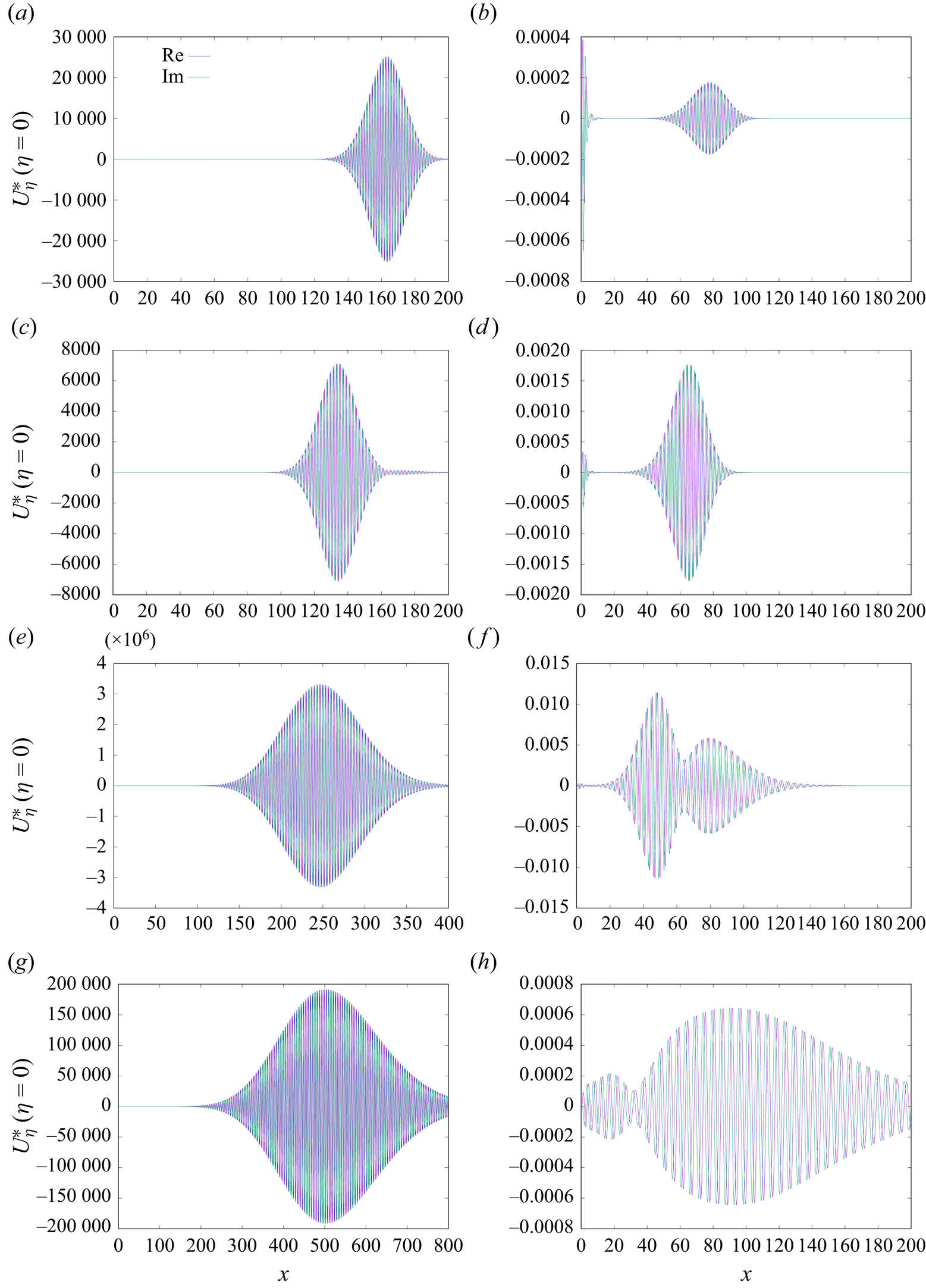
Figure 1. Downstream development of  $U^*_\eta (\eta =0)$ for
  $M_\infty =0,1,2,5$,
  $\beta =0.01$ and
  $0.02$. Panels show (a)
  $\beta =0.01$,
  $M_\infty =0$, (b)
  $\beta =0.02$,
  $M_\infty =0$, (c)
  $\beta =0.01$,
  $M_\infty =1$, (d)
  $\beta =0.02$,
  $M_\infty =1$, (e)
  $\beta =0.01$,
  $M_\infty =2$, ( f)
  $\beta =0.02$,
  $M_\infty =2$, (g)
  $\beta =0.01$,
  $M_\infty =5$, (h)
  $\beta =0.02$,
  $M_\infty =5$.
Although these results are undoubtedly mathematically ‘rigorous’, properly taking into account non-parallel-flow effects, nonetheless, it is often (including in DS) useful to consider local stability analysis based upon a parallel-flow approximation, which is expected to become increasingly accurate/less heuristic further downstream. This is the theme of the following section.
4. Local stability analysis based upon a parallel-flow approximation
The previous section clearly indicates the strong potential for downstream growth (followed by decay) of disturbances. To elucidate this phenomenon further, we adopt a locally parallel approach (which is ad hoc in nature, with  $x$ serving as a parameter) to the (spatial) stability analysis. In particular, we write (where
  $\mathrm {Re}\{\nu \} >0$ indicates downstream growth of disturbances)
 $$\begin{align}
&(U^*(x,\eta),V^*(x,\eta),W^*(x,\eta),\varTheta^*(x,\eta),T^*(x,\eta),\rho^*(x,\eta),\mu^*(x,\eta))\nonumber\\
&\quad ={\rm e}^{\nu
x}(U^{**}(\eta),V^{**}(\eta),W^{**}(\eta),\varTheta^{**}(\eta),T^{**}(\eta),\rho^{**}(\eta),\mu^{**}(\eta)),
\end{align}$$
$$\begin{align}
&(U^*(x,\eta),V^*(x,\eta),W^*(x,\eta),\varTheta^*(x,\eta),T^*(x,\eta),\rho^*(x,\eta),\mu^*(x,\eta))\nonumber\\
&\quad ={\rm e}^{\nu
x}(U^{**}(\eta),V^{**}(\eta),W^{**}(\eta),\varTheta^{**}(\eta),T^{**}(\eta),\rho^{**}(\eta),\mu^{**}(\eta)),
\end{align}$$and so leading on from (3.12)–(3.17)
 \begin{align} &\mathrm{i} x \rho^{**}+\bar U_0 \left(-\tfrac12 \eta \rho^{**}_\eta +x \nu \rho^{**}\right)-\tfrac12\eta U^{**}\bar\rho_{0\eta} +\bar \rho_0\left(-\tfrac12\eta U^{**}_\eta+x \nu U^{**}\right)-\tfrac12 \eta \rho^{**}\bar U_{0\eta} \nonumber\\ &\qquad +\rho^{**} \bar V_{0\eta} +\bar \rho_{0\eta} V^{**}+\rho^{**}_\eta\bar V_0+\bar\rho_0 V^{**}_\eta+\beta x \bar \rho_0 W^{**}=0, \\ &\bar\rho_0\left[\mathrm{i} xU^{**}+x\nu \bar U_0 U^{**}-\tfrac12\eta \bar U_0 U^{**}_\eta-\tfrac12\eta U^{**} \bar U_{0\eta}+\bar V_0 U^{**}_\eta+V^{**}\bar U_{0\eta}\right]\nonumber\\ &\qquad +\rho^{**}\left(-\tfrac12 \eta \bar U_0 \bar U_{0\eta}+\bar V_0 \bar U_{0\eta}\right)\nonumber \end{align}
 \begin{align} &\quad= \mu^{**}_\eta \bar U_{0\eta}+\bar\mu_{0\eta} U^{**}_\eta+\bar \mu_0 U^{**}_{\eta\eta} +\mu^{**} \bar U_{0\eta\eta}- x\beta^2 \bar \mu_0 U^{**}, \end{align}
 \begin{align} &-\mathrm{i} x \bar \rho_0 \varTheta^{**}+ \beta\rho^{**}\left[ \tfrac12 \bar U_0( \bar V_0+ \eta \bar V_{0\eta})-\bar V_0 \bar V_{0\eta}\right] \nonumber\\ &\qquad -\bar\rho_{0\eta}\left[\mathrm{i} x W^{**}+\bar U_0(x\nu W^{**}-\tfrac12\eta W^{**}_\eta)+\bar V_0 W^{**}_\eta\right]\nonumber\\ &\qquad-\bar \rho_0\left[\bar U_0\left(x\nu \varTheta^{**}-\tfrac12 \varTheta^{**}-\tfrac12\eta\varTheta^{**}_\eta\right)+\bar V_0\varTheta^{**}_\eta\right.\nonumber\\ &\qquad \left.+\,\varTheta^{**}\bar V_{0\eta}-\tfrac12 \beta U^{**}(\bar V_0+\eta \bar V_{0\eta})+\bar U_{0\eta}\left(x \nu W^{**}-\tfrac12 \eta W^{**}_\eta\right)\right] \nonumber\\ &\qquad+\bar \mu_{0\eta}(2 W^{**}_{\eta\eta}-2x\beta^2W^{**}-x\beta\nu U^{**}+\tfrac12 \beta\eta U^{**}_\eta)+\bar \mu_{0\eta\eta}(- \beta V^{**}+W^{**}_\eta)\nonumber\\ &\qquad +\bar \mu_0(\varTheta^{**}_{\eta\eta}-x\beta^2\varTheta^{**})-\bar U_{0\eta}(-\beta x \nu \mu^{**}+\tfrac12 \beta\eta \mu^{**}_\eta) + \beta\left(\tfrac12 \bar \mu_{0\eta}+\tfrac12 \eta \bar \mu_{0\eta\eta}\right)U^{**} \nonumber\\ &\qquad-2 \beta \mu_\eta^{**} \bar V_{0\eta}- \beta \mu^{**}\left({-}2 \bar V_{0\eta\eta}+\tfrac12 \bar U_{0\eta}+\tfrac12\eta \bar U_{0\eta\eta}\right)=0, \end{align}
 \begin{align} & \bar \rho_0\left[ \mathrm{i} x T^{**}+\bar U_0(x \nu T^{**}-\tfrac12 \eta T^{**}_\eta)-\tfrac12\eta \bar T_{0\eta} U^{**}+\bar V_0 T^{**}_{\eta} + \bar T_{0\eta} V^{**} \right]\nonumber\\ &\qquad +\rho^{**}\left(-\tfrac12\eta \bar T_{0\eta}\bar U_0+\bar V_0 \bar T_{0\eta}\right)\nonumber\\ &\quad=\frac{1}{\sigma} \left [ \bar \mu_{0\eta} T^{**}_\eta +\mu^{**}_\eta \bar T_{0\eta} +\bar \mu_0 T^{**}_{\eta\eta} +\mu^{**} \bar T_{0\eta\eta} -x \beta^2 \bar \mu_0 T^{**} \right ]\nonumber\\ &\qquad + (\gamma-1) M_\infty^2 \left( 2 \bar \mu_0\bar U_{0\eta}U^{**}_\eta +\mu^{**} \bar U^2_{0\eta} \right), \end{align}
 \begin{gather} \varTheta^{**}=W^{**}_\eta+\beta V^{**}, \end{gather}
 \begin{gather} \rho^{**} \bar T_0 +\bar \rho_0 T^{**}=0. \end{gather}
The above system was then discretised and initial estimates for the eigenvalues  $\nu$ were determined using a QZ algorithm, before being refined using a local search procedure. Here, as in DS, we focus our attention on what appears to be the single unstable mode. Our results are presented in figure 2. It should be pointed out that there was no evidence of unstable thermally driven (i.e. entropy) modes (although § 5.4 does indicate a slight caveat to this statement). Results are presented for growth rates
  $\mathrm {Re}\{\nu \}$ for free-stream Mach numbers 0, 1, 2 and 5 at downstream locations
  $x=100$, 200 and 400; these results are represented by the unstable regions of parameter space. As the free-stream Mach number increases, it can be observed that the peak growth rate occurs at progressively lower values of the wavenumber
  $\beta$, and the same trend is clear with increasing downstream location, together with an increasingly higher peak (although this can be anticipated from DS). Certainly, there is an indication of an increasingly intricate structure to the parameter space as compressibility effects are increased.

Figure 2. Locally parallel variation of spatial growth rates  $\mathrm {Re}\{\nu \}$ for
  $M_\infty =0,1,2,5$ with spanwise wavenumber
  $\beta$ at
  $x=100$ (blue),
  $x=200$ (green),
  $x=400$ (red); unstable regimes only shown. Panels show (a)
  $M_\infty =0$, (b)
  $M_\infty =1$, (c)
  $M_\infty =2$, (d)
  $M_\infty =5$.
Figure 3 shows the wall-normal distributions of the amplitude of the disturbance streamwise and cross-flow velocity components and of the temperature distributions for the case of  $M_\infty =5$ at
  $x=100$,
  $200$ and
  $400$ corresponding to the cross-flow wavelengths yielding the maximum streamwise growth rates (as indicated).

Figure 3. Wall-normal disturbance distributions at  $x=100$ (
 $\beta =0.0004$, blue),
  $x=200$ (
 $\beta =0.00025$, green),
  $x=400$ (
 $\beta =0.00015$, red),
  $M_\infty =5$. Panels show (a)
  $|U^{**}|$, (b)
  $|W^{**}|$, (c)
  $|T^{**}|$.
An alternative perspective of growth rates is presented in figure 4, which shows the downstream development for two selected values of  $\beta$, namely
  $0.005$ and
  $0.01$. Figures 2 and 4 suggest quite a complicated variation in parameter space (
 $x$,
$x$,  $\beta$ and
  $M_\infty$). However, it is quite clear that compressibility has a significant effect on growth rates, especially downstream. Taken together, figures 2–4 provide the motivation for the following section.

Figure 4. Downstream variation of growth rates,  $\beta =0.005$ and
  $0.01$. Panels show (a)
  $\beta =0.005$, (b)
  $\beta =0.01$.
5. The far-downstream limit
5.1. The case  $\beta =O(1/x$)

We now consider the far-downstream ( $x\to \infty$) limit to the system (4.2)–(4.5), using an asymptotically rigorous approach. We take
  $Y=O(1)$ to be the key transverse scale, and we assume
  $\beta =\hat \beta /x$,
  $\hat \beta =O(1)$, in line with the incompressible two-dimensional (2-D) analysis of Lam & Rott (Reference Lam and Rott1960) and Ackerberg & Phillips (Reference Ackerberg and Phillips1972) and the corresponding 3-D analysis of DS
 $$\begin{gather} U= \bar U_{0\eta} (0)Y/\sqrt{x} + \delta x^{{-}1/2} \left( {\rm e}^{- \hat\lambda x^{3/2}} {\rm e}^{\mathrm{i} t} \cos(\hat\beta Z/x) \tilde u(Y)+ {\rm c.c.} \right) +\cdots, \end{gather}$$
 $$\begin{gather}V= \tfrac12 \bar U_{0\eta}(0) Y^2/x^{3/2} + \delta \left( {\rm e}^{- \hat\lambda x^{3/2}} {\rm e}^{\mathrm{i} t} \cos(\hat\beta Z/x) \tilde v(Y)+\ {\rm c.c.} \right) +\cdots, \end{gather}$$
 $$\begin{gather}W= \delta x \left( {\rm e}^{- \hat\lambda x^{3/2}} {\rm e}^{\mathrm{i} t} \sin(\hat\beta Z/x) \tilde w(Y)+ {\rm c.c.} \right) +\cdots, \end{gather}$$
 $$\begin{gather}p_2= \delta x^2 \left({\rm e}^{- \hat\lambda x^{3/2}} {\rm e}^{\mathrm{i} t} \cos(\hat\beta Z/x) \tilde p_2(Y)+ {\rm c.c.} \right) +\cdots, \end{gather}$$
 $$\begin{gather}T= \bar T_0(0) + \delta \left( {\rm e}^{- \hat\lambda x^{3/2}} {\rm e}^{\mathrm{i} t} \cos(\hat\beta Z/x) \tilde T(Y)+ {\rm c.c.} \right) +\cdots, \end{gather}$$
 $$\begin{gather}\rho= \bar \rho_0(0) + \delta \left( {\rm e}^{- \hat\lambda x^{3/2}} {\rm e}^{\mathrm{i} t} \cos(\hat\beta Z/x) \tilde \rho(Y)+ {\rm c.c.} \right) +\cdots, \end{gather}$$
 $$\begin{gather}\mu = \bar \mu_0(0) + \delta \left( {\rm e}^{- \hat\lambda x^{3/2}} {\rm e}^{\mathrm{i} t} \cos(\hat\beta Z/x) \tilde \mu(Y)+ {\rm c.c.} \right) +\cdots. \end{gather}$$
In the above, we have chosen notation analogous to that used in DS, with  $\hat \lambda =-x^{-1/2}\nu$ (note that, in DS, the link between these two quantities had the incorrect factor
  $\tfrac {2}{3}$, although the ensuing results are correct and consistent with this paper). We then find that the
  $O(\delta )$ terms (at leading order in
  $x$) are
 $$\begin{gather} \mathrm{i} \tilde\rho-\tfrac32\hat\lambda \bar\rho_0(0)\tilde u-\tfrac32 \hat\lambda \bar U_{0\eta}(0)Y \tilde \rho +\bar\rho_0(0)\tilde v_Y +\hat\beta \bar\rho_0(0)\tilde w=0, \end{gather}$$
 $$\begin{gather}\mathrm{i} \bar\rho_0(0)\tilde u-\tfrac32 \hat\lambda \bar\rho_0(0)\bar U_{0\eta}(0) Y \tilde u + \bar U_{0\eta}(0)\bar \rho_0(0)\tilde v -\tilde \mu_Y \bar U_{0\eta}(0) -\bar \mu_0(0) \tilde u_{YY} =0, \end{gather}$$
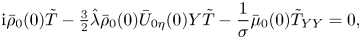 $$\begin{gather}\mathrm{i} \bar\rho_0(0)\tilde T-\tfrac32\hat\lambda \bar \rho_0(0) \bar U_{0\eta}(0) Y\tilde T -\frac{1}{\sigma}\bar \mu_0(0) \tilde T_{YY} =0, \end{gather}$$
 $$\begin{gather}\tilde p_{2 Y}=0, \end{gather}$$
 $$\begin{gather}\mathrm{i} \bar \rho_0(0)\tilde w -\tfrac32 \hat\lambda \bar \rho_0 (0) \bar U_{0\eta}(0)Y \tilde w -\hat\beta \tilde p_2 -\bar \mu_0 (0) \tilde w_{YY}=0, \end{gather}$$
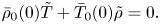 $$\begin{gather}\bar \rho_0 (0) \tilde T+\bar T_0(0)\tilde \rho=0. \end{gather}$$
Note that, just as in DS, algebraic terms of the form  $x^{\tau }$ multiply the exponential terms above, as described by Goldstein (Reference Goldstein1983) and Hammerton & Kerschen (Reference Hammerton and Kerschen1996), but these are only important at higher order, beyond that considered in this paper, and are omitted in the interests of brevity.
Before we discuss the solutions of (5.8)–(5.13) it is worth noting that the corresponding incompressible equations considered in DS, obtained by setting  $\tilde \mu =\tilde T=\tilde \rho =0$, admit analytical quasi-3-D solutions in terms of Airy functions. As pointed out by two referees, these were also discussed in Ricco & Wu (Reference Ricco and Wu2007).
It is useful to introduce  $\tilde \varTheta =\tilde w_Y$, and then to differentiate (5.12) with respect to
  $Y$, taking note of (5.11), yielding
 \begin{equation} \mathrm{i} \bar \rho_0(0)\tilde \varTheta -\tfrac32 \hat\lambda \bar \rho_0 (0) \bar U_{0\eta}(0) \tilde w -\tfrac32 \hat\lambda\bar \rho_0(0) \bar U_{0\eta}(0) Y\tilde \varTheta -\bar \mu_0 (0) \tilde \varTheta_{YY}=0. \end{equation}
 Note that the above eigenmodes can be loosely (sub-)classified into non-entropy and entropy modes. In the case of the former,  $\bar T \equiv \bar \rho \equiv 0$, whilst in the case of the latter, all components can in principle be triggered; we consider these non-entropy modes first, and defer a discussion of the entropy modes until § 5.4.
Now consider the overall compressible system, (5.8)–(5.13). Then, as discussed in the incompressible study of DS, when  $\hat \beta \ne 0$ it is necessary to consider two additional transverse scales in order to close the problem. A (further) useful point to note is that because of the homogeneous nature of (5.10), then for all non-entropy modes
  $\tilde T \equiv \tilde \mu \equiv \tilde \rho \equiv 0$, and so these outer regions assume very similar structure to the incompressible case with a relatively trivial adjustment to take account of the compressible nature of the base flow.
Note that as  $Y\to \infty$, in general
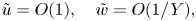 \begin{equation} \tilde u =O(1), \quad \tilde w=O(1/Y), \end{equation}
which is consistent with (5.8)–(5.12), and with connecting correctly to outer transverse regions, as described below. (We remark that these behaviours apply to the incompressible problem – there was a typographical error for  $\tilde w$ in (5.10) of DS.) A consideration of these outer regions is necessary to close the problem. In particular, we first consider the regime
  $\eta =Y/\sqrt {x}=O(1)$ (i.e. a longer wall-normal scale, indeed one that is comparable to the boundary-layer thickness itself). We then expect that (to leading order)
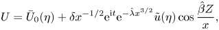 $$\begin{gather} U=\bar U_0(\eta)+\delta x^{{-}1/2 } \mathrm{e}^{\mathrm{i} t} \mathrm{e}^{-\hat\lambda x^{3/2 }}\tilde u(\eta)\cos \frac{\hat \beta Z}{x}, \end{gather}$$
 $$\begin{gather}V=x^{{-}1/2} \bar V_0(\eta)+\delta x^{1/2 } \mathrm{e}^{\mathrm{i} t} \mathrm{e}^{-\hat\lambda x^{3/2 }} \tilde v(\eta)\cos \frac{\hat \beta Z}{x} , \end{gather}$$
 $$\begin{gather}p_2=\delta x^2 \mathrm{e}^{\mathrm{i} t} \mathrm{e}^{-\hat\lambda x^{3/2 }}\tilde p_2(\eta) \cos \frac{\hat \beta Z}{x}, \end{gather}$$
 $$\begin{gather}W=\delta x^{1/2 } \mathrm{e}^{\mathrm{i} t} \mathrm{e}^{-\hat\lambda x^{3/2 }} \tilde w(\eta)\sin \frac{\hat \beta Z}{x}. \end{gather}$$
These lead to the following set of equations:
 $$\begin{gather} O(1): -\frac32 \hat\lambda \tilde u +\tilde v^{\prime}=0, \end{gather}$$
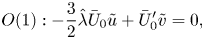 $$\begin{gather}O(1): -\frac32 \hat\lambda \bar U_0 \tilde u + \bar U_{0}^{\prime} \tilde v=0, \end{gather}$$
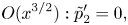 $$\begin{gather}O(x^{3/2 }): \tilde p_{2}^{\prime}=0, \end{gather}$$
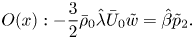 $$\begin{gather}O(x): -\frac32 \bar \rho_0 \hat\lambda \bar U_0 \tilde w =\hat \beta \tilde p_2. \end{gather}$$
These only differ in form from the corresponding incompressible analysis of DS, with the factor  $\bar \rho _0$ in the last equation. Thus, the solution of this system is
 $$\begin{gather} \tilde u = A \bar U_{0}^{\prime}(\eta), \end{gather}$$
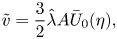 $$\begin{gather}\tilde v=\frac32 \hat\lambda A \bar U_0(\eta), \end{gather}$$
 $$\begin{gather}\tilde w={-}\frac{2\hat \beta \tilde p_2}{3\hat\lambda \bar U_0(\eta)\bar \rho_0(\eta)}, \end{gather}$$
which matches to the wall-layer solution as  $Y\to \infty$, where
  $A$ is a constant and clearly
  $\tilde p_2$ is a constant across this region.
If we now consider the region where  $\eta \gg 1$ (alternatively this can be regarded as the region wherein
  $\eta =O(\sqrt {x})$) then it is straightforward to see that the
  $V$ and
  $W$ perturbations are linked through the Cauchy–Riemann equations to yield
 $$\begin{gather} U=1+o(\delta \sqrt{x} {\rm e}^{-\hat\lambda x^{3/2}}) +\cdots , \end{gather}$$
 $$\begin{gather}V= x^{{-}1/2} \bar V_0(\infty)+\delta x^{1/2 } C \mathrm{e}^{\mathrm{i} t} \mathrm{e}^{-\hat\lambda x^{3/2 }} \mathrm{e}^{-({\eta\hat\beta}/{\sqrt{x}})}\cos \frac{\hat \beta Z}{x} +\cdots, \end{gather}$$
 $$\begin{gather}W=\delta x^{1/2 } C \mathrm{e}^{\mathrm{i} t} \mathrm{e}^{-\hat\lambda x^{3/2 }}\mathrm{e}^{-({\eta\hat\beta}/{\sqrt{x}})} \sin \frac {\hat \beta Z}{x} +\cdots, \end{gather}$$
 $$\begin{gather}p_2={-}\frac{3\delta C}{2\hat \beta} \hat\lambda x^2 \mathrm{e}^{\mathrm{i} t} \mathrm{e}^{-\hat\lambda x^{3/2 }} \mathrm{e}^{-({\eta\hat\beta}/{\sqrt{x}})}\cos \frac{\hat \beta Z}{x} +\cdots. \end{gather}$$
Here,  $C$ is a constant. The above implies that
 $$\begin{gather} C=\frac32 \hat\lambda A, \end{gather}$$
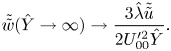
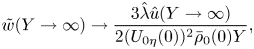 $$\begin{gather}\tilde w (Y \to \infty) \to \frac{3 \hat\lambda \hat u(Y \to \infty)}{2 (U_{0\eta}(0))^2 \bar \rho_0(0) Y}, \end{gather}$$
and this (now) works as a key boundary condition, which closes the problem, by augmenting (5.15a,b). This is another eigenvalue problem, for which standard numerical (finite-difference) methods were employed. Note that even when  $\hat \beta =0$, (5.32) indicates that the cross-flow (
 $\tilde w,\tilde \varTheta$) is still triggered by the 2-D mode. Note that the above system was ‘triggered’ in three distinct ways: (i) by forcing
  $\bar u_Y(Y=0)=1$; (ii) by forcing
  $\bar \varTheta (Y=0)=1$ (effectively 3-D non-entropy modes); (iii) by forcing
  $\bar T_Y(Y=0)$ or
  $\bar T(Y=0)=1$ (entropy modes).
Usefully, in the case of non-entropy modes (which of course captures the all-important unstable mode), the key system (5.8)–(5.14) can be scaled, resulting in (just) one parameter dependent on the Mach number (here, we therefore set  $\tilde T=\tilde \rho =\tilde \mu =0$ and implicitly assume that for
  $Y=O(1)$, generally
  $\tilde u=O(1)$). We write
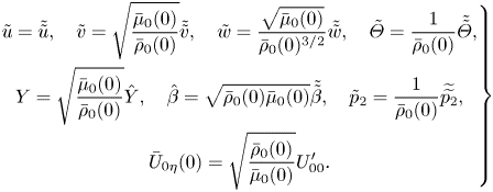 \begin{equation} \left. \begin{gathered} \tilde u = \tilde{\tilde{u}}, \quad \tilde v= \sqrt{\frac{\bar \mu_0(0)}{\bar \rho_0(0)}} \tilde{\tilde{v}}, \quad \tilde w = \frac{\sqrt{\bar\mu_0(0)}}{\bar \rho_0(0)^{3/2}} \tilde{\tilde{w}}, \quad \tilde\varTheta=\frac{1}{\bar \rho_0(0) } \tilde{\tilde{\varTheta}},\\ Y=\sqrt{\frac{\bar \mu_0(0)}{\bar \rho_0(0)}} \hat Y, \quad \hat\beta= \sqrt{\bar\rho_0(0)\bar\mu_0(0)} \tilde{\tilde{\beta}}, \quad \tilde p_2 = \frac{1}{\bar \rho_0(0) } \widetilde{\widetilde{p_2}},\\ \bar U_{0\eta}(0)= \sqrt{\frac{\bar\rho_0(0)}{\bar\mu_0(0)}} U_{00}^\prime. \end{gathered} \right\} \end{equation}
The net result arising from (5.8)–(5.13) is the following (simplified) eigen-system:
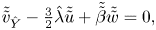 $$\begin{gather} \tilde{\tilde{v}}_{\hat Y} -\tfrac32 \hat\lambda \tilde{\tilde{u}} +\tilde{\tilde{\beta}} \tilde{\tilde{w}}=0, \end{gather}$$
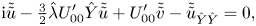 $$\begin{gather}\mathrm{i} \tilde{\tilde{u}} -\tfrac32 \hat\lambda U_{00}^\prime \hat Y \tilde{\tilde{u}} + U_{00}^\prime \tilde{\tilde{v}} -\tilde{\tilde{u}}_{\hat Y\hat Y} =0, \end{gather}$$
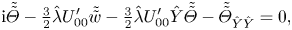 $$\begin{gather}\mathrm{i} \tilde{\tilde{\varTheta}} -\tfrac32 \hat \lambda U_{00}^\prime \tilde{\tilde{w}} -\tfrac32 \hat \lambda U_{00}^\prime \hat Y \tilde{\tilde{\varTheta}} -\tilde{\tilde{\varTheta}}_{\hat Y\hat Y} =0 , \end{gather}$$
 $$\begin{gather}\tilde{\tilde{\varTheta}}= \tilde{\tilde{w}}_{\hat Y}, \end{gather}$$
whilst the all-important far-field boundary condition (5.32) is now
 \begin{equation} \tilde{\tilde{w}}(\hat Y\to\infty) \to \frac{3\hat\lambda \tilde{\tilde{u}}}{2U_{00}^{\prime 2} \hat Y}. \end{equation}
 The results shown in figure 5 are confined to unstable regions, and correspondingly show the existence of a lower neutral point at lower values of the (scaled) spanwise wavenumber, whilst at higher wavenumbers, the modes remain unstable, but less so. Usefully, this system is precisely that found in the incompressible case of DS, but with one trivial difference, namely that  $\bar U_{0\eta }(0)$ is merely replaced by
  $U_{00}^\prime$, and so we can immediately write (using these previously published results) that in the limit as
  $\tilde {\tilde {\beta }} \to \infty$
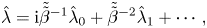 \begin{equation} \hat \lambda= \mathrm{i} \tilde{\tilde{\beta}}^{{-}1}\hat \lambda_0 + \tilde{\tilde{\beta}}^{{-}2} \hat\lambda_1 + \cdots, \end{equation}
where
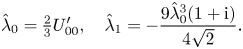 \begin{equation} \hat \lambda_0=\tfrac23 U_{00}^\prime, \quad \hat \lambda_1={-}\frac{9 \hat \lambda_0^3 (1+{\rm i})}{4 \sqrt{2}}. \end{equation}
Notice that, here, the effect of compressibility for these non-entropy modes is represented by just the one parameter, namely  $U_{00}^\prime$, whose value varies from circa
  $0.332$ in the case of incompressible flows to circa
  $0.376$ in the case of Sutherland's law with
  $C=0.5$, in particular, as
  $M_\infty \to \infty$ (adiabatic wall conditions). This benign behaviour is clearly seen in figure 6, and implies that
  $\hat \lambda$, for fixed
  $\tilde {\tilde {\beta }}$, is a relatively weak function of free-stream Mach number. In figure 7 there is a comparison between the (downstream-marching) numerical results for
  $\hat \beta =O(1)$ and the corresponding results as
  $\hat \beta \to \infty$, translating (5.39) into the corresponding variables for figure 5. For quite small values of the scaled wavenumber
  $\hat \beta$ there is some suggestion of the locally parallel results approaching the asymptotic results as
  $x$ increases), the agreement is frankly poor for larger values of
  $\hat \beta$. This discrepancy leads us on to the analysis of the following subsection, for the regime
  $\hat \beta =O(x^{1/2})$.


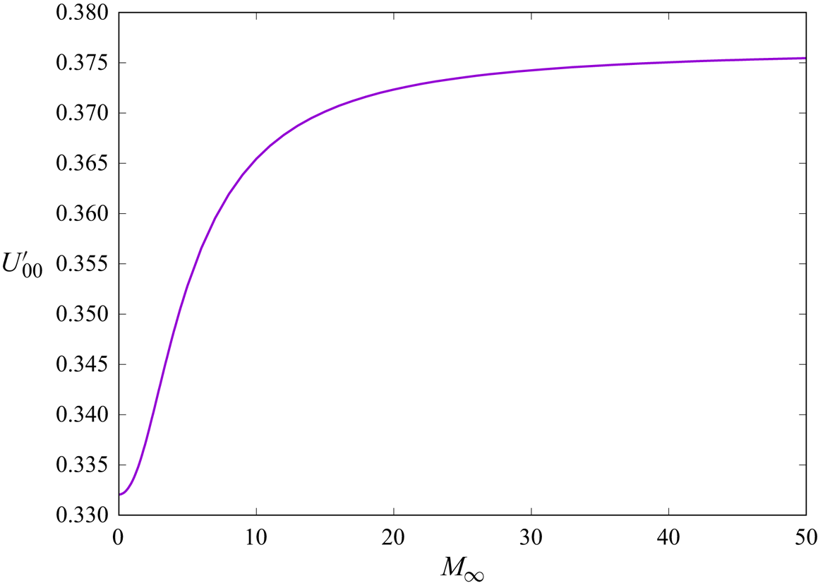
Figure 6. Variation of the compressibility parameter  $U_{00}^\prime$ with free-stream Mach number
  $M_{\infty }$ (adiabatic wall conditions).

Figure 7. Variation of  $\mathrm {Re}\{\hat \lambda \}$ with (scaled) spanwise wavenumber
  $\hat \beta$ for
  $M_\infty =5$ at
  $x=100$ (blue),
  $x=200$ (green),
  $x=400$ (red), all obtained using the locally parallel approach described in § 4. The dashed line corresponds to the
  $x\to \infty$ results obtained from (5.8)–(5.13).
5.2. Higher spanwise wavenumber disturbances – $\beta =O(x^{-1/2})$

The above strongly suggests the existence of an upper neutral point as the spanwise wavenumber is increased. This is also seen in the incompressible case of DS, but was not addressed in detail. Here, we go on to consider this aspect in rather more detail, and indeed reveal details about the instability of the flow in the compressible regime, not found in the incompressible regime. Although the  $\hat \beta \to \infty$ results indicate what amounts to neutral spatial stability, these shed no light on the behaviour of perturbations at (even) shorter wavelengths downstream. Partly guided by these results, we set
  $\beta =\beta ^*/x^{1/2}$, with
  $\beta ^* =O(1)$, and we expect when
  $Y=O(1)$
 $$\begin{gather} U= \bar U_{0\eta} (0)Y/\sqrt{x} + \delta x^{{-}1/2} \left({\rm e}^{ \nu x} {\rm e}^{\mathrm{i} t} \cos(\beta^* Z/x^{1/2}) \tilde u(Y)+{\rm c.c.}\right)+\cdots, \end{gather}$$
 $$\begin{gather}V= \tfrac12 \bar U_{0\eta}(0) Y^2/x^{3/2} + \delta \left({\rm e}^{ \nu x} {\rm e}^{\mathrm{i} t} \cos(\beta^* Z/x^{1/2}) \tilde v(Y)+{\rm c.c.}\right)+\cdots, \end{gather}$$
 $$\begin{gather}W= \delta x^{1/2} \left({\rm e}^{ \nu x} {\rm e}^{\mathrm{i} t} \sin(\beta^* Z/x^{1/2}) \tilde w(Y)+{\rm c.c.}\right)+\cdots, \end{gather}$$
 $$\begin{gather}p_2= \delta x \left({\rm e}^{ \nu x} {\rm e}^{\mathrm{i} t} \cos(\beta^* Z/x^{1/2}) \tilde p_2(Y)+{\rm c.c.}\right)+\cdots, \end{gather}$$
 $$\begin{gather}T=\bar T_0(0)+\delta \left( \mathrm{e}^{\mathrm{i} t} \mathrm{e}^{ \nu x}\tilde T(Y)\cos (\beta^* Z/ x^{1/2})+{\rm c.c.}\right)+\cdots, \end{gather}$$
 $$\begin{gather}\rho=\bar \rho_0(0)+\delta \left( \mathrm{e}^{\mathrm{i} t} \mathrm{e}^{ \nu x}\tilde \rho(Y)\cos ( \beta^* Z/ x^{1/2})+{\rm c.c.}\right)+\cdots, \end{gather}$$
 $$\begin{gather}\mu =\bar \mu_0(0)+\delta \left( \mathrm{e}^{\mathrm{i} t} \mathrm{e}^{ \nu x}\tilde \mu(Y)\cos ( \beta^* Z/ x^{1/2})+{\rm c.c.}\right)+\cdots. \end{gather}$$
The leading-order governing system (in  $\delta$) is then
 $$\begin{gather} \tilde v_Y + \beta^* \tilde w=0, \end{gather}$$
 $$\begin{gather}\bar\rho_0(0)( \mathrm{i} \tilde u + \bar U_0^{'}(0) \tilde v) -\bar \mu_0(0)\tilde u_{YY} =0, \end{gather}$$
 $$\begin{gather}\tilde p_{2}^{\prime}=0, \end{gather}$$
 $$\begin{gather}\bar\rho_0(0)\mathrm{i} \tilde w - \beta^* \tilde p_{2}-\bar \mu_0(0)\tilde w_{YY} =0, \end{gather}$$
 $$\begin{gather}\bar\rho_0(0)\mathrm{i}\tilde T + \bar T_{0\eta}(0)\tilde v-\frac{\bar \mu_0(0)}{\sigma} \tilde T_{YY} =0. \end{gather}$$
 The main points to glean from this system are the behaviours as  $Y\to \infty$. We find that
 \begin{equation} \left. \begin{gathered} \tilde w \to -\frac{\mathrm{i} \beta^* \tilde p_2}{\bar\rho_0(0)}, \quad \tilde v \to \frac{\mathrm{i} \beta^{*2} Y\tilde p_2}{\bar\rho_0(0)} -\frac{(1+\mathrm{i})\beta^{*2}(\bar\mu_0(0))^{1/2}\tilde p_2}{\sqrt{2} (\bar\rho_0(0))^{3/2}} ,\\ \tilde u \to -\frac{\beta^{*2} Y \bar U_0^\prime (0)\tilde p_2}{\bar\rho_0(0)} +\frac{(1-\mathrm{i})\beta^{*2}(\bar\mu_0(0))^{1/2}\tilde p_2 \bar U_0^\prime(0)}{\sqrt{2}(\bar\rho_0(0))^{3/2}}. \end{gathered} \right\} \end{equation}
 The primary region is when  $\eta =O(1)$, as strongly suggested by our
  $\hat \beta \to \infty$ results. The resulting scalings are then
 $$\begin{gather} U=\bar U_0(\eta)+\delta \left( \mathrm{e}^{\mathrm{i} t} \mathrm{e}^{ \nu x}\tilde u(\eta)\cos \frac{\beta^* Z}{x^{1/2}}+{\rm c.c.}\right)+\cdots, \end{gather}$$
 $$\begin{gather}V=x^{{-}1/2} \bar V_0(\eta)+\delta x^{1/2 }\left( \mathrm{e}^{\mathrm{i} t} \mathrm{e}^{\nu x} \tilde v(\eta)\cos \frac{\beta^* Z}{x^{1/2}}+{\rm c.c.}\right)+\cdots , \end{gather}$$
 $$\begin{gather}p_2=\delta x \left( \mathrm{e}^{\mathrm{i} t} \mathrm{e}^{\nu x}\tilde p_2(\eta) \cos \frac{\beta^* Z}{x^{1/2}}+{\rm c.c.}\right)+\cdots, \end{gather}$$
 $$\begin{gather}W=\delta x^{1/2 } \left( \mathrm{e}^{\mathrm{i} t} \mathrm{e}^{\nu x} \tilde w(\eta)\sin \frac{\beta^* Z}{x^{1/2}}+{\rm c.c.}\right)+\cdots, \end{gather}$$
 $$\begin{gather}T=\bar T_0(\eta)+\delta \left( \mathrm{e}^{\mathrm{i} t} \mathrm{e}^{ \nu x}\tilde T(\eta)\cos \frac{\beta^* Z}{x^{1/2}}+{\rm c.c.}\right)+\cdots, \end{gather}$$
 $$\begin{gather}\rho=\bar \rho_0(\eta)+\delta \left( \mathrm{e}^{\mathrm{i} t} \mathrm{e}^{ \nu x}\tilde \rho(\eta)\cos \frac{\beta^* Z}{x^{1/2}}+{\rm c.c.}\right)+\cdots. \end{gather}$$
 The resulting (key) system as  $x \to \infty$ is then
 $$\begin{gather} (\mathrm{i}+\nu \bar U_0) \tilde\rho + \bar \rho_0\nu \tilde u +\bar \rho_{0\eta} \tilde v+\bar \rho_0 \tilde v_{\eta} +\beta^* \bar \rho_0 \tilde w=0, \end{gather}$$
 $$\begin{gather}(\mathrm{i} +\nu \bar U_0)\tilde u+\bar U_{0\eta}\tilde v=0, \end{gather}$$
 $$\begin{gather}\bar\rho_0 (\mathrm{i}+ \nu \bar U_0) \tilde v +\tilde p_{2}^{\prime}=0, \end{gather}$$
 $$\begin{gather}\bar \rho_0 (\mathrm{i}+ \nu \bar U_0) \tilde w -\beta^* \tilde p_2=0, \end{gather}$$
 $$\begin{gather}(\mathrm{i} +\nu \bar U_0 )\tilde T + \bar T_{0\eta}\tilde v=0. \end{gather}$$
Putting everything together, then the above may be combined to yield
 \begin{equation} \tilde p_{2\eta\eta}-\beta^{*2} \tilde p_2+ \left( \frac{\bar T_{0\eta}}{\bar T_0} -\frac{2 \nu \bar U_{0\eta}} {\mathrm{i}+\nu \bar U_0}\right)\tilde p_{2\eta} =0, \end{equation}
which is basically the compressible Rayleigh equation, with zero streamwise wavenumber. In order to match on to the  $Y=O(1)$ region correctly, we must have
 \begin{equation} \tilde p_{2\eta}(\eta=0)=0, \end{equation}
along with, as  $\eta \to \infty$
 \begin{equation} \tilde p_{2\eta}+ \beta^* \tilde p_2 \to 0. \end{equation}
Although computations exclusively confined to the real  $\eta$-axis can yield reasonably accurate results for unstable modes, this is not the case for damped and neutral modes. This issue was overcome by diverting the computations into the complex
  $\eta$-plane. Specifically we took integration paths of the following form: starting at the origin
  $\eta =0$, the computations headed towards
  $\eta =(\xi _0,0)$, then up to
  $\eta =(\xi _0,\zeta _0)$, then along to
  $\eta =(\xi _1,\zeta _0)$, back down to
  $\eta =(\xi _1,0)$, then along to
  $\eta =(\xi _{max},0)$. Typically, we took
  $\xi _0=0.05$,
  $\zeta _0=2$ and
  $\xi _1=40$, although our results were confirmed by adjusting these values. Of course the base (compressible Blasius-type) flow requires evaluation in complex
  $\eta$ space, but this is straightforward. This procedure yielded results for
  $\nu$ in good agreement with the finite
  $x$ calculations, as illustrated in the next subsection. This technique is reminiscent of the Mack (Reference Mack1984) procedure for tackling Rayleigh's equation for compressible boundary-layer stability calculations (for example). The effects of the Mach number on the solutions for
  $\mathrm {Re}(\nu )$ are shown in figure 8. The incompressible case is stable, (a result that may be anticipated from DS) while at higher Mach numbers instability is found, with growth rates that increase as the Mach number increases, and with maximum growth rates moving towards smaller values of
  $\beta ^*$. These results also indicate the existence of an upper (with respect to
  $\beta ^*$) neutral point.


5.3. Comparison of asymptotic results with streamwise developing results
As a particularly stringent test of the asymptotic results described in the previous subsection, we compare these with the (notional) spatial growth rates as computed from the downstream-marching procedure, as described in § 3. Specifically, we took the local wall shear stress results as shown in figure 1(h), for  $\beta =0.02$,
  $M_\infty =5$ and evaluated
  $U^*_{\eta x}(\eta =0)/U^*_\eta (\eta =0)$ (numerically). The results for the effective growth rate, based on the streamwise perturbation wall shear (
 $\mathrm {Re}\{\nu \}$) are shown in green in figure 9. (Note that the corresponding distribution for the wall temperature clearly indicated damping.) For comparison, results corresponding to figure 5 are shown in blue, where results for varying values of
  $\hat \beta$ have been translated into varying values of downstream location
  $x$, corresponding to fixed
  $\beta$. Similarly, results corresponding to figure 8 are shown in purple, where results for varying values of
  $\beta ^*$ have been translated into varying values of downstream location
  $x$, corresponding to fixed
  $\beta$. Taking the downstream-marching/spatially developing results of § 3 as a benchmark, we see that there is reasonable agreement with the
  $\beta =O(1/x)$ results from § 3, but this deteriorates further downstream. On the other hand, comparison of this benchmark with the
  $\beta =O(1/\sqrt {x})$ of § 5.2 is poor for smaller values of downstream location
  $x$, but this improves further downstream. In some ways, this result is not unexpected given the different regimes considered in the first two subsections of this section, but nonetheless is encouraging.


5.4. Entropy modes
Computations using both the locally parallel approach of § 3 and the far-downstream approach of § 5.1 strongly suggested that entropy modes, i.e. those initiated by triggering the temperature field, were all stable, decaying downstream. Indeed, it is noteworthy that with the scaling of  $\beta$, not only is (5.10) homogeneous, it is also independent of scaled spanwise wavenumber. Closer inspection of the energy equation (4.5) in particular highlights that for entropy modes, in the far-downstream limit, the original
  $\beta =O(1)$ remains the key spanwise scaling, with
  $Y=O(1)$ being the important transverse scaling. The leading terms are notionally
  $O(x)$, and lead to the homogeneous form
 \begin{equation} \bar \rho_0(0)\left( \mathrm{i} -\tfrac32 \hat \lambda \bar U_{0\eta}(0) Y \right ) T^{**}-\frac{\bar \mu_0(0)}{\sigma} \left (T^{**}_{YY} - \beta^2 T^{**} \right) =0, \end{equation}
the solution of which is
 \begin{equation} T^{**}= \hat \kappa_1{\rm{Ai}}(Y^*), \end{equation}
where
 \begin{equation} Y^*=\left(-\frac{3\sigma \hat \lambda \bar\rho_0(0) \bar U_{0\eta}(0)}{2 \bar \mu_0(0)}\right)^{1/3}\left(Y- \frac{\mathrm{i}\bar \rho_0(0)+\beta^2 \bar\mu_0(0)/\sigma}{\tfrac32 \bar\rho_0(0)\hat\lambda \bar U_{0\eta}(0)}\right). \end{equation}
In the adiabatic case
 \begin{equation} \hat\lambda=\frac{\sqrt{2\sigma} (1+\mathrm{i})}{3 \bar \rho_0(0) \bar U_{0\eta}(0)(\bar\mu_0(0))^{1/2} (\rho_n^\prime)^{3/2}} \left (\bar\rho_0(0)-\mathrm{i} \beta^2 \bar\mu_0(0)/\sigma \right)^{3/2}, \end{equation}
where the  $\rho _n^{\prime }$ corresponds to the
  $n$th zero of the derivative of the Airy function, viz.
 \begin{equation} {\rm{Ai}}^{\prime}(-\rho_n^{\prime}) =0, \end{equation}
which replicates the incompressible 2-D eigenvalues with no cross-flow and zero spanwise wavenumber, as discussed in DS.
On the other hand, for specified wall temperature flows
 \begin{equation} \hat\lambda=\frac{\sqrt{2\sigma} (1+\mathrm{i})}{3 \bar \rho_0(0) \bar U_{0\eta}(0)(\bar\mu_0(0))^{1/2} (\rho_n)^{3/2}} \left (\bar\rho_0(0)-\mathrm{i}\beta^2 \bar\mu_0(0)/\sigma \right)^{3/2}, \end{equation}
where the  $\rho _n$ corresponds to the
  $n$th zero of the Airy function per se, viz.
 \begin{equation} {\rm{Ai}}(-\rho_n) =0. \end{equation}
Note that this also replicates the incompressible modes with cross-flow and with zero spanwise wavenumber, also discussed by DS. These can be regarded as entropy modes, and these are present, even as  $M_\infty \to 0$.
Close inspection of the real part of  $\hat \lambda$ from above indicates that these modes are always damped modes, in line with our remarks above. However, as a caveat, reverting to the downstream development approach of § 3, now triggering the perturbation through wall forcing of the temperature field (in particular by specifying a wall-normal temperature gradient for the perturbation flow) leads to an interesting possibility. Figure 10 shows the resulting downstream development of the perturbation wall shear for the zero Mach number case, with
  $\beta =0.01$. Note that upstream of
  $x\approx 120$, there was little flow response, but thereafter there is a significant response. Intriguingly, in the regime of significant flow field response, the temperature field response (not shown) is insignificant, and rapidly diminishes downstream. In this case, however, the non-parallel nature of the flow leads to full interaction between the temperature and flow fields, the latter being triggered by the former, which then leads to downstream growth. This does highlight the fact that whilst local stability analyses based upon a parallel-flow approximation can be useful, they can also overlook important effects of non-parallelism.
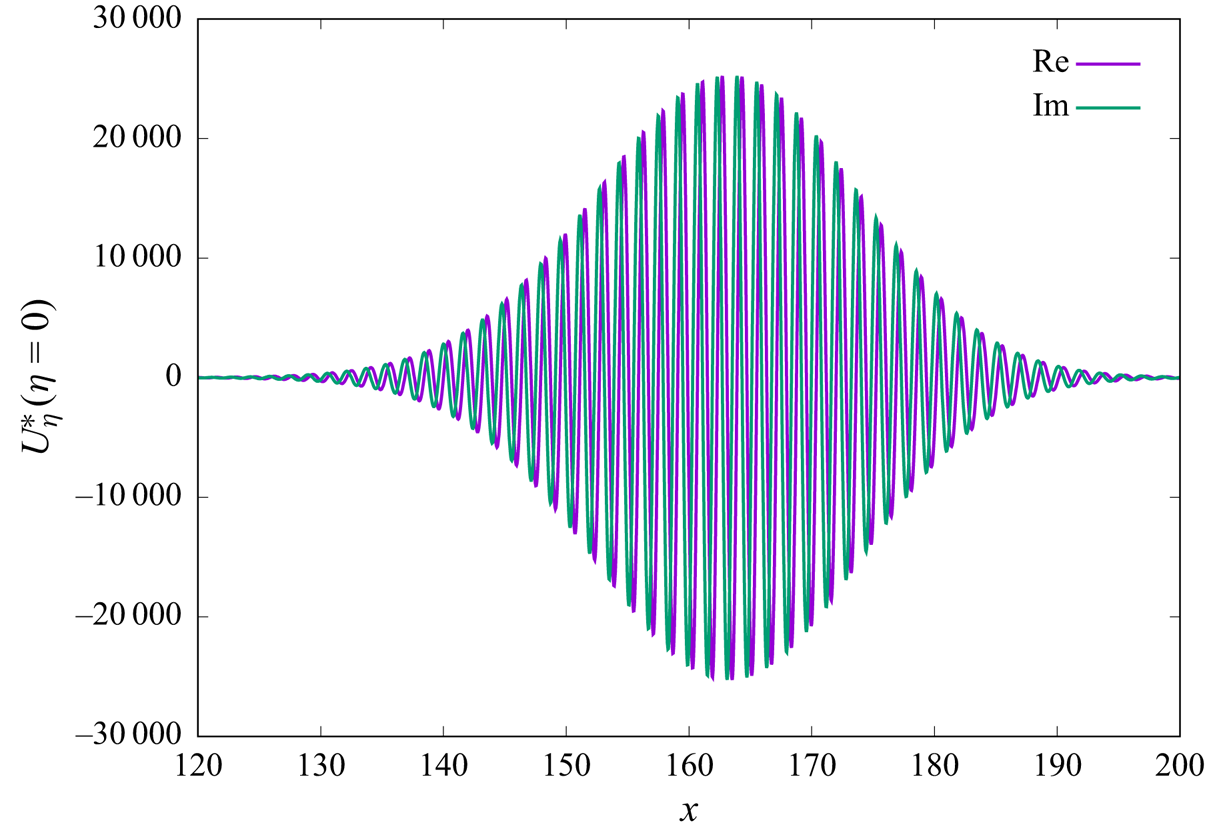
Figure 10. Downstream development of streamwise perturbation wall shear  $U^*_\eta (\eta =0)$ triggered by wall temperature forcing for
  $M_\infty =0$ and
  $\beta =0.01$.
6. Conclusions
We have considered solutions of the unsteady, compressible BRE, following on from the incompressible study of DS. Our focus has been on disturbances with spanwise wavelength comparable to the boundary-layer thickness (and on adiabatic wall conditions, although it would be a simple matter to change the analysis to other wall conditions). Thus, the resulting governing equations are the unsteady (time-periodic), compressible BRE. These are solved using several approaches. In the first, the flow field develops downstream (for fixed spanwise wavenumbers). These results show that growth, followed by decay of disturbances can occur (similar to the results of DS). However, particularly at higher Mach numbers, results suggest that after one regime of decay, a second regime exists, wherein growth is observed, followed by decay again. A local stability analysis based upon a parallel-flow approximation is undertaken, and this confirms the potential for downstream growth. This leads on to asymptotic analyses of the stability modes, far downstream, which confirm the presence of instabilities. A further wavenumber regime is also considered, wherein the spanwise wavenumber is  $O(x^{-1/2})$ and this suggests that a further regime of instability (inviscid in nature) can occur as the free-stream Mach number increases. This could account for the aforementioned second growth regime, found at higher Mach numbers.
One interesting observation, found in the case of entropy modes is that although the locally parallel approaches predict stability, when non-parallelism is properly taken into account as in § 3, the interaction between thermal and non-thermal effects can trigger the latter, and as a consequence instabilities.
Our numerical and asymptotic results suggest that the effects of compressibility should not be ignored in future studies of unsteady three-dimensional eigensolutions in boundary-layer flow. The importance of entropy modes can be significant; although in the context of locally parallel-flow approximations these are all damped, if non-parallelism is taken into account, these damped modes can trigger downstream growth though coupling between thermal and hydrodynamic fluctuations. In addition, as in the incompressible case, consideration of a link with the unstable modes described here and compressible Klebanoff modes should be investigated, although the latter modes are induced by free-stream turbulence. The studies of Ricco & Wu (Reference Ricco and Wu2007), Ricco et al. (Reference Ricco, Tran and Ye2009) and Marensi et al. (Reference Marensi, Ricco and Wu2017), amongst others, have investigated the effect of compressibility on these low-frequency streaks in compressible boundary layers. These streaks are located at the edge of the boundary layer while the unsteady eigensolutions considered in the current study reside close to the wall in the boundary layer.
Finally, this paper does suggest the possibility of modes of instability, not reported in the past. Asymptotic analysis, such as implemented in this paper, takes on what may be regarded as a microscopic view of physical parameter space, that could perhaps be overlooked by DNS studies, and as a consequence there is an interesting possibility for such studies to search in the parameter regimes identified in this paper, for behaviours that we have reported.
Acknowledgements
The authors are grateful to the referees for their detailed comments which helped to improve this manuscript.
Funding
P.W.D. acknowledges the Sydney Mathematical Research Institute (SMRI) for funding for a visitorship and its hospitality, where some of early parts of this research were conducted.
Declaration of interests
The authors report no conflict of interest.


 Open access