


1. Introduction
The creation of zonal flow in the planetary atmosphere is a spectacular example of the self-organization in physical systems (Charney Reference Charney1971; Hasegawa Reference Hasegawa1985). There is a strong analogy between the geostrophic turbulence and the electrostatic turbulence of a magnetized plasma in the plane perpendicular to an ambient magnetic field. Because the generation of zonal flow (coherent structure) affects the turbulent transport in magnetized plasmas, how strong it can be is of great interest in the context of plasma confinement (Diamond et al. Reference Diamond, Itoh, Itoh and Hahm2005). The aim of this work is to estimate exact lower bounds on the ‘zonal enstrophy’, which hence must be satisfied regardless of the dynamics, and elucidate how the lower bounds are determined; lower bounds on the zonal enstrophy indicate that the zonal flow must be stronger than the given value.
The inverse-cascade model explains the essence of the self-organization process. Because of the approximate two-dimensional geometry (due to the scale separation between the shallow vertical direction and wide horizontal directions), the vortex dynamics is free from the stretching effect. Then, the energy of flow velocity tends to accumulate into large-scale vortices, while the enstrophy (the norm of vorticity) cascades to small scales (Kraichnan Reference Kraichnan1967). On a rotating sphere, the gradient of the Coriolis force yields the Rossby-wave term in the vortex dynamics equation, which brings about latitude/longitude anisotropy, and the large-scale vorticity forms zonal flow (Charney Reference Charney1971). The nonlinear term driving the inverse cascade becomes comparable to the linear Rossby-wave term at the Rhines scale, which gives a crude estimate of the latitudinal size of the zonal flow (Rhines Reference Rhines1975).
While the inverse-cascade model illustrates the general tendency of a nonlinear process, the underlying mechanism requires more detailed analysis. The modulational instability plays an essential role in exciting the energy transfer in the wavenumber space (Lorentz Reference Lorentz1972; Gill Reference Gill1974; Connaughton et al. Reference Connaughton, Nadiga, Nazarenko and Quinn2010). In addition to the energy and enstrophy, another quadratic integral is known to be an adiabatic invariant (only changes by fourth order of perturbations) in the zonal-flow domain of wavenumber space, restricting the energy transfer there (Balk, Nazarenko & Zakharov Reference Balk, Nazarenko and Zakharov1991; Balk Reference Balk1991, Reference Balk2005). Various numerical simulations have been done to demonstrate the creation of zonal flow. Two different categories of models must be distinguished; one is the unforced, free decaying turbulence, and the other is the forced, quasi-stationary turbulence. In the latter case, the interaction between the mean flow and the turbulence (Farrell & Ioannou Reference Farrell and Ioannou2007; Bakas & Ioannou Reference Bakas and Ioannou2011; Srinivasan & Young Reference Srinivasan and Young2012) or inhomogeneous vorticity mixing (Dritschel & McIntyre Reference Dritschel and McIntyre2008; Scott & Dritschel Reference Scott and Dritschel2012) has been found to be a causal mechanism of zonal-flow generation. For these forced, quasi-stationary cases, one has to include some dissipation mechanism for large-scale flows in order to remove the energy accumulating in the large-scale regime by the inverse cascade. The usual viscosity only works for short-scale flows, so something like ‘friction’ is added to the model (however, which mechanism works in a realistic planetary system is still controversial). For the free decaying case, early simulation results (Vallis & Maltrud Reference Vallis and Maltrud1993; Yoden & Yamada Reference Yoden and Yamada1993; Yoden et al. Reference Yoden, Ihioka, Hayashi and Yamada1999) demonstrated the self-organization of zonal flow, and found that the scale of the zonal flow is similar to that of Rhines’ estimate. However, the quantitative comparison between the Rhines scale and the zonal-flow scale was left unclear. On the other hand, in the forced turbulence case, a more complex relation has been found, because of the influence of the dissipation mechanism for large-scale flows (see Williams Reference Williams1978; Danilov & Gurarie Reference Danilov and Gurarie2002; Sukoriansky, Dikovskaya & Galperin Reference Sukoriansky, Dikovskaya and Galperin2007).
In parallel with simulation studies, there have been theoretical attempts to nail down the ‘target’ of the spontaneous process, i.e. formulating a variational principle that reveals what the dynamics tends to reach. This can be done by identifying the target functional to be minimized (or maximized) as well as the constraints that restrict admissible candidates. A well-known example is the entropy maximization in a microcanonical ensemble (the constraints are total particle number and total energy), which gives the Gibbs distribution. In the application to field theories, where we have to deal with infinite-dimensional phase spaces, we encounter the problem of ultraviolet catastrophe (which must be removed by appropriate quantization, see Ito & Yoshida (Reference Ito and Yoshida1996)). Suspending such subtle problems, formal calculations have been made to obtain the thermal equilibrium distribution of flow fields. In the context of the planetary atmosphere, the statistical equilibrium state in the two-dimensional incompressible Euler system was studied in Miller (Reference Miller1990) and Robert & Sommeria (Reference Robert and Sommeria1991). In Turkington et al. (Reference Turkington, Majda, Haven and Dibattista2001), the maximum entropy distribution over the ensemble constrained by total energy and circulation was compared with the large-scale vortex structures observed on Jupiter. However, because of the essential non-equilibrium property of turbulence (as the cascade model is based on ‘dissipation’ in the Kolmogorov micro-scales, one has to assume a ‘driving force’ to maintain the (quasi-) stationary state, or consider a transient process of free decay), the entropy may not be an effective tool to dictate the self-organization.
There is a different type of approach guided by the notion of selective dissipation (Hasegawa Reference Hasegawa1985). The Taylor state of a magneto-fluid (Taylor Reference Taylor1974, Reference Taylor1986) is the prototype of such a model of self-organization, which minimizes the magnetic field energy ( $E = ({1}/{2}) \int |\boldsymbol {B}|^2\,\mathrm {d}^3x = ({1}/{2}) \int |\boldsymbol {\nabla }\times \boldsymbol {A}|^2\,\mathrm {d}^3x$, where
  $\boldsymbol {B}=\boldsymbol {\nabla }\times \boldsymbol {A}$ is the magnetic field and
  $\boldsymbol{A}$ is the vector potential) under the constraint on the magnetic helicity (
 $H=({1}/{2}) \int \boldsymbol {A}\boldsymbol {\cdot }\boldsymbol {B}\,\mathrm {d}^3x$). The reason why
  $E$ is more fragile than
  $H$ is because
  $E$ includes another differential operator curl in the integrand. This model explains the relaxed states of magnetized plasmas in various systems, ranging from laboratory experiments to astronomical objects. Regarding the two-dimensional turbulence in the planetary atmosphere, the minimization of the generalized enstrophy (see Proposition 2.1) under the constraint on the energy has been studied to show that the solution of the minimization problem predicts a steady state with streamlines parallel to contours of the topography (Bretherton & Haidvogel Reference Bretherton and Haidvogel1976). Although these two stories, i.e. the energy–helicity relation in the magneto-fluid and the enstrophy–energy relation in the two-dimensional (2-D) fluid appear to be parallel (as Hasegawa (Reference Hasegawa1985) describes in the unified vision), there is a fundamental difference when viewed from their Hamiltonian structures, and the latter needs a careful interpretation. In both systems, the ideal constants (the helicity in magneto-fluids and the enstrophy in 2-D fluids) are Casimirs, by which the orbits are constrained on the level sets of these constants (Morrison Reference Morrison1998). In the magneto-fluid phase space, the orbits converge into the equilibrium point as the energy diminishes; the minimum energy (Hamiltonian) state, on each level set of the helicity, gives an equilibrium point. In the 2-D fluid system, however, the level set of the enstrophy is not embedded as a smooth submanifold in the topology of the energy norm (because the enstrophy is a fragile quantity, its level set looks like a fractal set; see Appendix A). Hence, we have to reverse the role of the Hamiltonian (energy) and the Casimir (enstrophy), and minimize the enstrophy for a given energy. Then, the critical point is not necessarily an equilibrium point. In this specific problem, however, it happens to be so, because it is the ‘maximum point’ of the energy. Notice that the minimization of the enstrophy under a constrained energy is equivalent to the maximization of the energy under a constrained enstrophy (see Appendix A). The maximization of the energy appears to be consistent with the inverse-cascade story. However, the simultaneous process, i.e. the forward cascade of the enstrophy, violates the constancy of the enstrophy. The dual aspects of the 2-D turbulence pose a paradox in the mechanical interpretation of the selective dissipation.
The target of this study is totally different. Whereas we formulate a variational principle using the list of ideal constants of motion, the target functional is not selected from them. We estimate the minimum of the enstrophy possibly given to the zonal component (which we call the zonal enstrophy). Knowing how strong the zonal flow must be and how it is controlled is an important issue in the study of turbulent transport. While the total enstrophy is an ideal constant of motion, the zonal part alone is not. We are not proposing that the zonal enstrophy is selectively dissipated; we never provide the target functional with the role of dictating dissipation process. Our target functional is simply what we want to estimate. We derive an a priori estimate of the zonal enstrophy, which must apply to every possible dynamics under a set of prescribed conditions; the ideal invariants are used as such constraints (we do not include the adiabatic invariant, because it needs the wavenumber information that is not amenable to our formulation). The actual dynamics is the second subject to be explored, which will be the task of § 5. The analogy of quantum mechanical energy levels may be helpful to explain our perspective. When we want to estimate the energy of an orbital electron, the variational principle to find the critical values of energy, for a fixed total probability, leads us to the eigenvalue problem for the Hamiltonian. The actual energy level that a particular electron will take is determined, for example, by the de-excitation process of emitting photons. We will find a similar picture for the 2-D-fluid turbulence; the zonal enstrophy has discrete levels of critical values (local minima); by emitting wavy enstrophy, the zonal enstrophy relaxes into lower levels.
If there is no constraint on partitioning, the zonal enstrophy can be minimized to zero (even if the total enstrophy is kept at a non-zero constant). But some constraints prevent this occurring. We will identify the ‘key constraints’ that determine a reasonable estimate of the zonal enstrophy.
The reciprocal problem, which maximizes the complementary wavy enstrophy (= total enstrophy  $-$ zonal enstrophy), was first studied by Shepherd (Shepherd Reference Shepherd1988) with a different motivation, i.e. to estimate upper bounds on instabilities in the nonlinear regime. This is seemingly equivalent to the minimization of the zonal component, however, the effective ‘constraints’ may differ (see Appendix A). The conservation of the pseudo-momentum was invoked as the essential constraint. Improved estimates have been proposed by taking into account more general set of invariants which are known as Casimirs (Ishioka & Yoden Reference Ishioka and Yoden1996). In the present study of the minimization of the zonal component, however, we invoke a different constant of motion, the energy, as the principal constraint (in addition to other ones such as the impulse). The physical reason is clear because the self-organization is a spontaneous process in which the redistribution of the enstrophy between the zonal and wavy components can occur only if the energetics admits. Moreover, the energy constraint imparts a mathematically peculiar property to the variational principle, which is the other incentive of this study.
In the next section, we will start by reviewing the basic formulation and preliminaries. Section 4 describes the main result. We will derive discrete levels of the minimum zonal enstrophy. We will propose the notion of de-excitation to lower enstrophy levels (in analogy to energy levels of quantum states); the relaxation into lower levels corresponds to the inverse cascade. According to the conjecture of the Rhines scale (Rhines Reference Rhines1975), the inverse cascade continues until the linear Rossby-wave term overcomes the nonlinear term. In § 5, we will study the relaxation process by numerical simulation. The conventional Rhines scale will be revisited to give an improved estimate of the relaxed zonal enstrophy level. Section 6 concludes this paper.
2. Governing equations
2.1. Vortex dynamics on a beta plane
We consider a barotropic fluid on a beta-plane
 \begin{equation} M = \{\boldsymbol{\xi}=(x,y)^{\mathrm{T}} ;\, x\in[0,1), y\in (0,1) \}. \end{equation}
Here,  $\boldsymbol{\xi}$ is the coordinate while
  $x$ is the azimuthal coordinate (longitude) and
  $y$ is the meridional coordinate (latitude). The aspect ratio of the domain does not influence the results of Theorems 4.1 and 4.2 (see § 5.1), so we consider a unit square domain. We are using the standard single-layer beta-channel model of geophysical fluid dynamics on the unit square, with periodic boundary conditions in the zonal
  $x$-direction and no-flux boundary conditions in the meridional
  $y$-direction. Without loss of generality, we work in a reference frame in which the net zonal mass flux vanishes. We will denote the standard
  $L^2$ inner product by
  $\langle f,g \rangle$
 \begin{equation} \langle f,g \rangle = \int_M f(\boldsymbol{\xi}) g(\boldsymbol{\xi}) \,\mathrm{d}^2\xi, \end{equation}
and the  $L^2$ norm by
  $\| f\| = \langle f, f\rangle ^{1/2}$. Here, f and g are arbitrary functions.
The state vector is the fluid vorticity  $\omega \in L^2(M)$. We define the streamfunction (or Gauss potential)
  $\psi$ by
 \begin{equation} -\varDelta\psi = \omega , \end{equation}
where  $\varDelta =\partial _x^2 + \partial _y^2$. The flow velocity is given by
 \begin{equation} \boldsymbol{v}=\left( \begin{array}{@{}c@{}} v_x \\ v_y \end{array}\right) = \boldsymbol{\nabla}_\perp\psi = \left( \begin{array}{@{}c@{}} \partial_y \psi \\ -\partial_x \psi \end{array}\right) . \end{equation}
Taking into account the Coriolis force, the governing equation of  $\omega$ is
 \begin{equation} \partial_t \omega + \{\omega + \beta y, \psi \} =0, \end{equation}
where  $\{ f, g \} = (\partial _x\kern0.05em f )(\partial _y g) - (\partial _x g)(\partial _y\kern0.05em f)$, and
  $\beta$ is a real constant number measuring the meridional variation of the Coriolis force. When
  $\beta =0$, (2.5) reduces into the standard vorticity equation. A finite
  $\beta$ introduces anisotropy to the system, resulting in the creation of zonal flow. The Rhines scale (Rhines Reference Rhines1975) speaks of the balance of the two terms
  $\{\omega , \psi \}$ and
  $\{ \beta y, \psi \}$, by which we obtain the typical scale length of the zonal flow (see § 4.5).
Inverting (2.3) by  $\mathcal {K}=(-\varDelta )^{-1}$, we may rewrite (2.5) as
 \begin{equation} \partial_t \omega + \{\omega + \beta y, \mathcal{K} \omega \} =0. \end{equation}
We call
 \begin{equation} \omega_t := \omega + \beta y \end{equation}
the total vorticity, which is the sum of the fluid part  $\omega$ and the ambient part
  $\beta y$ (the latter is due to the rotation of the system).
The following identity will be useful in the later calculations:
 \begin{equation} \langle f, \{ g,h \} \rangle = \langle g, \{ h, f \} \rangle, \end{equation}
where  $f, g$ and
  $h$ are
  $C^1$-class functions in
  $M$, and either
  $f$ or
  $g$ satisfy the boundary conditions.
2.2. Conservation laws and symmetries
Proposition 2.1 (constants of motion)
The following functionals are constants of motion of the evolution equation (2.6):
(i) Energy
(2.9)By rewriting \begin{equation} E(\omega) :=\tfrac{1}{2} \langle \omega, \mathcal{K}\omega \rangle . \end{equation}(2.10)we find that\begin{equation} E= \tfrac{1}{2} \langle (-\varDelta\psi), \psi \rangle =\tfrac{1}{2} \int_M |\boldsymbol{\nabla}\psi|^2\,\mathrm{d}^2 \xi =\tfrac{1}{2} \int_M |\boldsymbol{\nabla}_\perp\psi|^2\,\mathrm{d}^2 \xi = \tfrac{1}{2} \int_M |\boldsymbol{v}|^2\,\mathrm{d}^2 \xi, \end{equation}$E$ evaluates the kinetic energy of the flow $\boldsymbol {v}$.
(ii) Longitudinal momentum
(2.11)We may rewrite\begin{equation} P(\omega) := \int_M \partial_y ( \mathcal{K}\omega) \,\mathrm{d}^2 \xi . \end{equation}(2.12)to see that\begin{equation} P=\int_M \partial_y\psi \,\mathrm{d}^2 \xi =\int_M v_x\,\mathrm{d}^2 \xi, \end{equation}$P$ is the integral of the longitudinal momentum. Considering the boundary conditions, $P$ must be constantly zero.(iii) Circulation
(2.13)Integrating by parts, we may write\begin{equation} F (\omega) :=\langle 1 , \omega \rangle . \end{equation}(2.14)which evaluates the circulation of the flow\begin{equation} F = \int^1_0 \left[ v_x \right]^{y=1}_{y=0} \, \mathrm{d}x, \end{equation}$\boldsymbol {v}$ along the boundary $\partial M$.(iv) Impulse
(2.15)Integrating by parts and using the boundary conditions, we may rewrite\begin{equation} L(\omega) :=\langle y, \omega \rangle . \end{equation}(2.16)The first term on the right-hand side is\begin{equation} L = \int_M y (\partial_x v_y -\partial_y v_x)\,\mathrm{d}^2\xi = \int_M v_x\,\mathrm{d}^2\xi - \int_0^1 \left[\, y v_x \,\right]_{y=0}^{y=1}\,\mathrm{d}x. \end{equation}$P$, which vanishes by the boundary condition. Hence, $L$ corresponds to the angular momentum $\boldsymbol {\xi }\times \boldsymbol {v}$ averaged over the boundary.(v) Generalized enstrophy
(2.17)where\begin{equation} G_\beta(\omega) :=\int_M f(\omega+\beta y)\,\mathrm{d}^2\xi, \end{equation}$f$ is an arbitrary $C^1$-class function, and the argument $\omega +\beta y$ is the total vorticity including the ambient term $\beta y$. For $f(u)=u^2/2$, $G_\beta (\omega )$ is the conventional enstrophy of the total vorticity.(vi) Fluid enstrophy
(2.18)\begin{equation} {Q}(\omega) := \tfrac{1}{2} \| \omega \|^2 . \end{equation}


3. Zonal and wavy components
The phase space of the vorticity  $\omega$ is
 \begin{equation} {V} = L^2(M). \end{equation}
We say that  $\omega$ is zonal when
  $\partial _x \omega \equiv 0$ in
  $M$. The totality of zonal flows defines a closed subspace
  ${V}_z \subset {V}$. The zonal average
 \begin{equation} \mathcal{P}_z \omega := \int_0^1 {\omega}(x,y)\,\mathrm{d}x \end{equation}
may be regarded as a projection from  ${V}$ onto
  ${V}_z$. By the orthogonal decomposition
  $V = V_z \oplus V_w$, we define the orthogonal complement
  ${V}_w$, i.e.
  ${\omega }_w \in {V}_w$, iff
  $\langle {\omega }_w, \omega _z\rangle = 0$ for all
  $\omega _z\in {V}_z$. We call
  ${\omega }_w \in {V}_w$ a wavy component, which has zero zonal average:
  $\mathcal {P}_z \omega _w = 0$. We will denote
 \begin{equation} \mathcal{P}_w = I- \mathcal{P}_z , \end{equation}
which is the projector onto  $V_w$. Now we may write
 \begin{equation} V = V_z \oplus V_w = (\mathcal{P}_z V) \oplus (\mathcal{P}_w V). \end{equation}
The following basic properties may be known to the reader, but we summarize them as Lemmas for the convenience of the analysis in § 4:
Lemma 3.1 (partition laws)
Let us decompose  $\omega = \omega _z + \omega _w (\omega _z = \mathcal {P}_z \omega \in V_z, \omega _w = \mathcal {P}_w\omega \in V_w)$.
(i) The circulation and the impulse are occupied by the zonal component
$\omega _z$, i.e.
(3.5)\begin{gather} F(\omega) = F(\omega_z), \end{gather}(3.6)\begin{gather} L(\omega) = L(\omega_z). \end{gather}(ii) Quadratic invariants such as the fluid enstrophy and the energy are separated without any mixture terms as
(3.7)\begin{gather} {Q}(\omega) = {Q}(\omega_z) + {Q}(\omega_w), \end{gather}(3.8)\begin{gather} E(\omega) = E(\omega_z) + E(\omega_w) . \end{gather}


4. Estimate of zonal enstrophy
4.1. Zonal enstrophy versus wavy enstrophy
The aim of this work is to find the minimum of the zonal enstrophy defined by
 \begin{equation} Z(\omega) := \tfrac{1}{2} \| \mathcal{P}_z \omega \|^2 . \end{equation}
The complementary wavy enstrophy is  ${W}(\omega ) = ({1}/{2}) \| \mathcal {P}_w \omega \|^2$. By (3.7), the total enstrophy is
 \begin{equation} {Q}(\omega) = {Q}(\mathcal{P}_z\omega) + {Q}(\mathcal{P}_w\omega) = Z(\omega) + {W}(\omega). \end{equation}
When the total enstrophy  ${Q}(\omega )$ is conserved (see Proposition 2.1(v)), the minimum of
  $Z(\omega )$ gives the maximum of
  ${W}(\omega )$.
The simplest version of the minimization problem is to find the minimum  $Z(\omega )$ under the constraint of
  ${Q}(\omega )=C_Q (\neq 0)$. Introducing a Lagrange multiplier
  $\nu$, we minimize
 \begin{equation} Z(\omega)-\nu {Q}(\omega) . \end{equation}
Using the self-adjointness of  $\mathcal {P}_z$, we obtain the Euler–Lagrange equation
 \begin{equation} \mathcal{P}_z \omega -\nu \omega =0. \end{equation}
Operating  $\mathcal {P}_z$ on (4.4) yields
 \begin{equation} (1-\nu) \mathcal{P}_z\omega =0. \end{equation}
On the other hand, operating  $\mathcal {P}_w$ yields
 \begin{equation} \nu \mathcal{P}_w\omega =0. \end{equation}
There are two possibilities for solving these simultaneous equations.
(i) If
$\nu =0$ then, $\mathcal {P}_z\omega =\omega _z=0$ and $\mathcal {P}_w\omega =\omega _w$ is an arbitrary function satisfying ${Q}(\omega _w)=C_Q$; hence, $\mathrm {min}\,Z(\omega )=0$. (This simple exercise reveals an unusual aspect of the present variational principle, which is caused by the non-coerciveness of the functional $Z(\omega )$ to be minimized. Notice that the minimizer is not unique, because $\mathcal {P}_z$ has non-trivial kernel, i.e. $\mathrm {Ker}(\mathcal {P}_z) = V_w$).(ii) If
$\nu =1$ then, $\mathcal {P}_w\omega =\omega _w=0$ and $\mathcal {P}_z\omega =\omega _z$ is an arbitrary function satisfying ${Q}(\omega _z)=Z(\omega )=C_Q$; hence, this solution gives the ‘maximum’ of $Z(\omega )$.


As we mentioned above, the minimizer is not unique here. To obtain a non-trivial estimate of the minimum  $Z(\omega )$, we have to take into account ‘constraints’ posed on the dynamics of redistributing enstrophy. Guided by Proposition 2.1, we start with some simple ones.
4.2. Constraints by circulation and impulse
Let us consider the circulation and impulse as constraints.
Theorem 4.1 The minimizer of the zonal enstrophy  $Z(\omega )$ under the constraints on the circulation
  $F(\omega )=C_F$, the impulse
  $L(\omega )=C_L$, as well as the total enstrophy
  ${Q}(\omega )=C_Q$ is a vorticity
  $\omega$ such that
 \begin{equation} \mathcal{P}_z \omega = a + b y , \quad (a =4C_F - 6 C_L,\ b=12 C_L - 6 C_F), \end{equation}
which gives
 \begin{equation} Z_0 := \min Z(\omega) = 2C_F^2 - 6 C_F C_L + 6 C_L^2. \end{equation}
Proof. Let us minimize
 \begin{equation} Z(\omega) - \nu {Q}(\omega) - \mu_0 F(\omega)-\mu_1 L(\omega). \end{equation}
The Euler–Lagrange equation is
 \begin{equation} \mathcal{P}_z \omega - \nu \omega =\mu_0 + \mu_1 y. \end{equation}
Operating  $\mathcal {P}_z$ on both sides of (4.10) yields
 \begin{equation} (1-\nu) \mathcal{P}_z\omega =\mu_0 + \mu_1 y. \end{equation}
On the other hand, operating  $\mathcal {P}_w$ yields
 \begin{equation} \nu \mathcal{P}_w\omega=0. \end{equation}
First, assume that  $1-\nu \neq 0$. Inserting
  $\mathcal {P}_z\omega$ of (4.11) into the definition of
  $F(\omega )=F(\mathcal {P}_z\omega )$ and
  $L(\omega )=L(\mathcal {P}_z\omega )$ (see Lemma 3.1(i) and (ii)), we determine
  $\mu _0$ and
  $\mu _1$ to match the constraint
  $\langle 1 , \omega \rangle ={C_F}$ and
  $\langle y , \omega \rangle ={C_L}$; we obtain
  $a:= \mu _0/(1-\nu )=4C_F - 6 C_L$, and
  $b:=\mu _1/(1-\nu ) = 12 C_L - 6 C_F$. Inserting this
  $\omega _z = a + b y$ into
  $Z(\omega )$, we obtain the minimum (4.8). On the other hand, (4.12) is satisfied by
  $\nu =0$ (consistent with the forgoing assumption
  $1-\nu \neq 0$) and an arbitrary
  $\omega _w = \mathcal {P}_w\omega$ such that
 \begin{equation} \tfrac{1}{2} \| \omega_w\|^2 = C_Q -(2C_F^2 - 6 C_F C_L + 6 C_L^2) . \end{equation}
The right-hand side is non-negative, if the constraints  $F(\omega )=C_F$,
  $L(\omega )={C_L}$ and
  ${Q}(\omega )=C_Q$ are consistent. It is only when the constants
  $C_F$,
  $C_L$ and
  $C_Q$ are given so that the right-hand side of (4.13) is zero, that the other assumption
  $1-\nu =0$ applies; then, the unique solution
  $\mathcal {P}_w\omega =0$ (hence,
  $\omega =\mathcal {P}_z\omega$) is obtained.
Notice that the minimizer is still non-unique (excepting the special case mentioned in the proof); every  $a + b y + \omega _w$ (
 $\forall \omega _w\in V_w$ such that (4.13) holds) satisfies (4.7). However, the minimum value (4.8) is uniquely determined.
4.3. Constraint by energy
The situation changes dramatically when we include the energy constraint  $E(\omega )=C_E$; a laminated vorticity distribution, epitomizing the structure of zonal flow, is created by the energy constraint. The meridional mode number of the zonal flow is identified by the ‘eigenvalue’ of the Euler–Lagrange equation, which specifies the ‘level’ of the zonal enstrophy (in analogy to the quantum number of discrete energy in quantum mechanics). To highlight the role of the energy constraint, we first omit the constraints on the circulation and impulse.
Taking into account the energy and total enstrophy constraint, we seek the critical points of
 \begin{equation} Z(\omega) - \nu Q (\omega) - \mu_2 E(\omega). \end{equation}
The Euler–Lagrange equation is
 \begin{equation} \mathcal{P}_z \omega - \nu \omega - \mu_2 \mathcal{K}\omega = 0. \end{equation}
Operating  $\mathcal {P}_z$ yields (denoting
  $\omega _z = \mathcal {P}_z\omega$)
 \begin{equation} \omega_z - \nu \omega_z - \mu_2 \mathcal{K}\omega_z = 0. \end{equation}
On the other hand,  $\omega _w = \mathcal {P}_w\omega$ must satisfy
 \begin{equation} \nu \omega_w + \mu_2 \mathcal{K}\omega_w = 0. \end{equation}
Putting  $\omega _z = -\partial _y^2 \psi _z(y)$ in (4.16), we obtain
 \begin{equation} \partial_y^2 \psi_z + \lambda^2 \psi_z = 0 , \quad \lambda^2 =\frac{\mu_2}{1-\nu} . \end{equation}
The solution satisfying the boundary conditions  $\psi _z(0)=\psi _z(1)=0$ is
 \begin{equation} \psi_z = A \sin \lambda y, \end{equation}
with eigenvalues
 \begin{equation} \lambda = n_1 {\rm \pi}\ (n_1 \in \mathbb{Z}). \end{equation}
The corresponding zonal vorticity is
 \begin{equation} \omega_z = A \lambda^2 \sin \lambda y . \end{equation}
On the other hand, putting  $\omega _w = -\varDelta \psi _w$, (4.17) reads
 \begin{equation} \varDelta \psi_w + k^2 \psi_w = 0 , \quad k^2 ={-}\frac{\mu_2}{\nu}. \end{equation}
The solution satisfying the boundary conditions  $\psi _w(x, 0)=\psi _w(x, 1)=0$, as well as the periodicity in
  $x$, is given by
 \begin{equation} \psi_w = B \sin k_x x \ \sin k_y y , \quad k^2=k_x^2+k_y^2 \end{equation}
with eigenvalues
 \begin{equation} k_x = 2 n_2 {\rm \pi}, \quad k_y = n_3 {\rm \pi}\, (n_2,\ n_3 \in \mathbb{Z}) . \end{equation}
The corresponding wavy vorticity is
 \begin{equation} \omega_w = B k^2 \sin k_x x \, \sin k_y y . \end{equation}
Summing the zonal and wavy components, we obtain
 \begin{gather} \psi = A \sin \lambda y + B \sin k_x x \ \sin k_y y , \end{gather}
 \begin{gather} \omega = A \lambda^2 \sin \lambda y + B k^2 \sin k_x x \ \sin k_y y . \end{gather}
The two amplitudes  $A$ and
  $B$ are determined by the constraints
  $E(\omega )=C_E$ and
  $Q(\omega )=C_Q$; inserting (4.26) and (4.27) into the definitions of
  $E(\omega )$ and
  $Q(\omega )$, we obtain
 \begin{gather} C_E = \frac{A^2 \lambda^2}{4} + \frac{B^2 k^2}{8} , \end{gather}
 \begin{gather} C_Q = \frac{A^2 \lambda^4} {4}+ \frac{B^2 k^4} {8}. \end{gather}
Solving (4.28) and (4.29) for  $A$ and
  $B$, and inserting the solution into the zonal enstrophy
  $Z(\omega )$ and wavy enstrophy
  $W(\omega )$, we obtain the critical values
 \begin{gather} Z_{\lambda,\epsilon} = \frac{\lambda^2 C_E -\epsilon C_Q } {1 -\epsilon}, \end{gather}
 \begin{gather}W_{\lambda,\epsilon} = \frac{C_Q - \lambda^2 C_E} {1 - \epsilon}, \end{gather}
where  $\epsilon = \lambda ^2/k^2$, scaling the ratio of the wavelength of the zonal components to that of the wavy components. For
  $Z_{\lambda ,\epsilon }\geq 0$ and
  $W_{\lambda ,\epsilon }\geq 0$, there are two possibilities:
  $\epsilon \leq (\lambda ^2 C_E)/C_Q \leq 1$ or
  $\epsilon \geq (\lambda ^2 C_E)/C_Q \geq 1$. Here, the former regime of
  $\epsilon$ is relevant, because we assume that the wavy components have smaller scales in comparison with the zonal component (i.e.
  $\epsilon <1$). Then,
  $Z_{\lambda ,\epsilon }$ of (4.30) increases monotonically as
  $\epsilon$ decreases (or
  $k^2$ increases; see figure 1), and we have
 \begin{equation} \lim_{\epsilon \to 0} Z_{\lambda,\epsilon} = \lambda^2 C_E . \end{equation}
Notice that this limit gives the upper bound for  $Z(\omega )$ of the corresponding eigenvalue
  $\lambda$, which is achieved when the wavy component has the smallest scale
  $\epsilon \rightarrow 0$. For actual wavy components,
  $Z(\omega )$ takes a smaller value than
  $\lambda ^2 C_E$, i.e.
 \begin{equation} Z(\omega) \leq \lambda^2 C_E . \end{equation}


4.4. Constraints by energy, circulation, impulse and total enstrophy
Now we study the minimum of the zonal enstrophy  $Z(\omega )$ under all constraints of energy, circulation, impulse and total enstrophy. In contrast to the observation of § 4.3 (where the minimum of
  $Z(\omega )$ is not determined by the energy
  $C_E$), we will find that the minimum of
  $Z(\omega )$ is determined by the circulation
  $C_F$ and impulse
  $C_L$. In comparison with the result of § 4.2, however, we have a discrete set of enstrophy levels (each of which corresponds to a different mode number). Whereas they are due to the energy constraint,
  $Z(\omega )$ itself does not depend on the values of the energy
  $C_E$.
Introducing Lagrange multipliers, we seek the minimizer of
 \begin{equation} Z(\omega) - \nu Q(\omega) - \mu_0 F(\omega) -\mu_1 L(\omega) - \mu_2 E(\omega). \end{equation}
The Euler–Lagrange equation is
 \begin{equation} \mathcal{P}_z \omega - \nu \omega -\mu_0 -\mu_1 y - \mu_2 \mathcal{K}\omega = 0. \end{equation}
The solution satisfying the boundary conditions  $\psi (x,0)=\psi (x,1)=0$, as well as the periodicity in
  $x$, is
  $\psi =\psi _z + \psi _w$ with
 \begin{gather} \psi_z = A_1 \cos \lambda y + A_2 \sin \lambda y - \frac{\mu_0 + \mu_1 y}{\mu_2} , \end{gather}
 \begin{gather}\psi_w = B \sin k_x x \ \sin k_y y , \end{gather}
where
 \begin{equation} \lambda=\sqrt{\frac{\mu_2}{1-\nu}}, \quad k^2 =k_x^2 +k_y^2 ={-}\frac{\mu_2}{\nu} , \end{equation}
and
 \begin{equation} k_x = 2 n_2 {\rm \pi}, \quad k_y = n_3 {\rm \pi}\, (n_2,\ n_3 \in \mathbb{Z}). \end{equation}
The corresponding vorticities are
 \begin{gather} \omega_z = A_1 \lambda^2 \cos \lambda y + A_2 \lambda^2 \sin \lambda y. \end{gather}
 \begin{gather}\omega_w = B k^2 \sin k_x x \ \sin k_y y . \end{gather}
The zonal enstrophy  $Z(\omega )$ of the minimizer is
 $$\begin{gather} Z(\omega) = \frac{A_1^2 \lambda^3}{8} (2 \lambda + \sin 2 \lambda) + \frac{A_2^2 \lambda^3}{8} (2 \lambda - \sin 2 \lambda) \nonumber\\ + \frac{A_1 A_2 \lambda^3}{4} (1 - \cos 2 \lambda). \end{gather}$$
 We have yet to determine the eigenvalue  $\lambda$ and the coefficients
  $A_1$,
  $A_2$ and
  $B$. Inserting
  $\psi =\psi _z+\psi _w$ and
  $\omega =\omega _z+\omega _w$ into the constraints
  $F(\omega )=C_F$,
  $L(\omega )=C_L$,
  $E(\omega )=C_E$, and
  $Q(\omega )=C_Q$, we obtain
 \begin{gather} C_F =A_1 \lambda \sin \lambda + A_2 \lambda (1- \cos \lambda) , \end{gather}
 \begin{gather}C_L = A_1 (\lambda \sin \lambda+ \cos \lambda- 1) + A_2 (\sin \lambda- \lambda \cos \lambda), \end{gather}
 \begin{gather}C_E = \frac{A_1^2 \lambda}{8} (2 \lambda + \sin 2 \lambda) + \frac{A_2^2 \lambda}{8} (2 \lambda - \sin 2 \lambda) \nonumber\\ + \, \frac{A_1 A_2 \lambda}{4} (1 - \cos 2 \lambda) - \frac{A_1 C_F}{2} \nonumber\\ \qquad \qquad \qquad \quad - \, \frac{[A_1 (\cos \lambda - 1) + A_2 \sin \lambda] C_L}{2} + \frac{B^2 k^2}{8},\end{gather}
 \begin{gather}C_Q = \frac{A_1^2 \lambda^3}{8} (2 \lambda + \sin 2 \lambda) + \frac{A_2^2 \lambda^3}{8} (2 \lambda - \sin 2 \lambda) \nonumber\\ \quad + \, \frac{A_1 A_2 \lambda^3}{4} (1 - \cos 2 \lambda) + \frac{B^2 k^4}{8}. \end{gather}
We may write (4.43) and (4.44) as
 \begin{equation} \left( \begin{array}{@{}c@{}} C_F \\ C_L \end{array} \right) = \boldsymbol{\mathsf{D}}(\lambda) \left( \begin{array}{@{}c@{}} A_1 \\ A_2 \end{array} \right). \end{equation}
with
 \begin{equation} \boldsymbol{\mathsf{D}}(\lambda) := \left( \begin{array}{@{}cc@{}} \lambda \sin \lambda & \lambda (1- \cos \lambda) \\ \lambda \sin \lambda+ \cos \lambda- 1 & \sin \lambda- \lambda \cos \lambda \end{array} \right) . \end{equation}
For given  $C_F$ and
  $C_L$, we solve (4.47) to determine the amplitudes of zonal vorticity
 \begin{gather} A_1 = \frac{C_F (\sin \lambda - \lambda \cos \lambda) + C_L (-\lambda + \lambda \cos \lambda)}{\mathrm{det}{D}(\lambda)}, \end{gather}
 \begin{gather}A_2 = \frac{C_F (-\lambda \sin \lambda - \cos \lambda + 1) + C_L \lambda \sin \lambda}{\mathrm{det}{D}(\lambda)}, \end{gather}
where  $\mathrm {det}{D}(\lambda ) = \lambda (2 - \lambda \sin \lambda - 2 \cos \lambda )$. Inserting (4.49) and (4.50) into (4.42), we obtain the zonal enstrophy evaluated as a function of
  $\lambda$, which we denote by
  $Z_\lambda$. The critical points (local minima) of
  $Z(\omega )$, given by
 \begin{equation} \frac{\mathrm{d}}{\mathrm{d}\lambda}Z_\lambda = 0, \end{equation}
determine the eigenvalues  $\lambda$ characterizing the enstrophy levels.
Instead of displaying the lengthy expression of  $Z_\lambda$, we will show its graphs for typical choices of the parameters
  $C_F$ and
  $C_L$. Notice that
  $Z_\lambda$ depends only on
  $C_F$ (circulation) and
  $C_L$ (impulse); it does not contain
  $C_E$ (energy) and
  $C_Q$ (enstrophy) as parameters. First, we pay attention to the singularities given by
  $\mathrm {det}{D}(\lambda )=0$, where
  $A_1 \to \infty$ and
  $A_0 \to \infty$, hence
  $Z_\lambda \to \infty$ (there is an exception, as discussed later). We show the graph of
  $\mathrm {det}{D}(\lambda )$ in figure 2.

Figure 2. The graph of  $\mathrm {det}{D}$.
There are two types of solutions
 \begin{equation} \lambda= \left\{ \begin{array}{@{}l} \varLambda_{2n}=2 n {\rm \pi},\\ \varLambda_{2n+1}= (2n+1){\rm \pi} - \delta_n , \end{array} \right. \quad (n=0, 1, \ldots), \end{equation}
where each  $\delta _n$ is a small positive number such that
  $\delta _n \rightarrow 0$ as
  $n\rightarrow \infty$. The minima of
  $Z_\lambda$ appear in every interval
  $(\varLambda _{2n}, \varLambda _{2n+1})$. However, if
  $C_F = 2 C_L$,
  $Z_\lambda$ remains finite at
  $\lambda = \varLambda _{2n+1}$. In this special case, the minima of
  $Z_\lambda$ appear in intervals
  $(\varLambda _{2n}, \varLambda _{2n+2})$.
In figure 3, we show examples of  $Z_\lambda$ calculated for (3a)
  $C_F=0.28$ and
  $C_L=0.07$, (3b)
  $C_F=0.28$ and
  $C_L=0.14$ (
 $C_F = 2 C_L$).

Figure 3. The graph of the critical zonal enstrophy  $Z_\lambda$ as a function of
  $\lambda$. The minima of
  $Z_\lambda$ determine the eigenvalues of
  $\lambda$. The points on the curve indicate the eigenvalues. We assume (a)
  $C_F=0.21$ and
  $C_L=0.0525$, and (b)
  $C_F=0.21$ and
  $C_L=0.105$.
At  $\lambda =0$,
  $Z_\lambda$ reproduces the result of Theorem 4.1, i.e.
 \begin{equation} \lim_{\lambda \to 0} Z_\lambda = Z_0=2C_F^2 - 6 C_F C_L + 6 C_L^2, \end{equation}
which is the absolute minimum of the zonal enstrophy under the constraints on the circulation  $F(\omega )=C_F$, the impulse
  $L(\omega )=C_L$ and the total enstrophy
  ${Q}(\omega )=C_Q$.
The role of the energy constraint  $E(\omega )=C_E$ is to create eigenvalues of
  $\lambda$ at which
  $Z_\lambda$ takes local minimum values. However, the value of
  $C_E$ does not influence the value of
  $Z_\lambda$ directly. As we have seen in (4.33), it poses a constraint on the maximum
 \begin{equation} Z(\omega) \leq \lambda^2 C_E, \end{equation}
in addition to the other implicit constraint  $Z(\omega )\leq C_Q$. Instead of the zonal component
  $\omega _z$ of (4.40),
  $C_E$ and
  $C_Q$ work for determining the complementary wavy component
  $\omega _w$ of (4.41). By (4.45) and (4.46), we obtain
 \begin{gather} k^2 = \frac{C_Q-Z_\lambda}{C_E-E_{z,\lambda}} , \end{gather}
 \begin{gather}B^2 = \frac{8(C_E-E_{z,\lambda})^2}{C_Q-Z_\lambda}, \end{gather}
where  $E_{z,\lambda }$ is the energy of the zonal component
  $\omega _z$ evaluated at the eigenvalue
  $\lambda$. Notice that
  $k^2 B^2$ (
 $\sim$ energy of the wavy component) is determined only by
  $C_E$ and
  $E_{z,\lambda }$. So, the role of the total enstrophy constraint is to determine the wavenumber
  $k$ of the wavy component.
For the special case of  $C_F=0$ and
  $C_L=0$, a laminated zonal flow (
 $A_1\neq 0$ and/or
  $A_2\neq 0$) can occur only if
 \begin{equation} \mathrm{det}{D}(\lambda) = \lambda (2 - \lambda \sin \lambda - 2 \cos \lambda) = 0. \end{equation}
Then, the eigenvalues are  $\lambda =\varLambda _{2n}$ and
  $\varLambda _{2n+1}$ (
 $n=0,1,2,\ldots$), the previous singular points; see figure 2. For
  $\lambda =\varLambda _{2n}$ (
 $\lambda =0$ gives the trivial solution
  $\omega _z=0$),
 \begin{equation} \boldsymbol{\mathsf{D}}(\lambda) = \left( \begin{array}{@{}cc@{}} 0 & 0 \\ 0 & - \lambda \end{array} \right), \end{equation}
hence,  $A_2=0$. On the other hand, for
  $\lambda =\varLambda _{2n+1}$,
 \begin{equation} \boldsymbol{\mathsf{D}}(\lambda) = \frac{1}{4} \lambda \sin \lambda \left( \begin{array}{@{}cc@{}} 4 & 2 \lambda \\ 2 & \lambda \end{array} \right) , \end{equation}
and then  $A_2 = -2 A_1/\varLambda _{2n}$. In both cases,
  $A_1$ is arbitrary, so we cannot determine the amplitude of the zonal vorticity
  $\omega _z$. Therefore, the trivial conditions
  $C_F=0$ and
  $C_L=0$ reproduce the situation of ‘no constraint’ discussed in § 4.3. We only have the estimate of the maximum (4.33).
The forgoing results are summarized as:
Theorem 4.2 For a given set of constants  $F(\omega )=C_F$,
  $L(\omega )=C_L$,
  $E(\omega )=C_E$ and
  ${Q}(\omega )=C_Q$, the zonal enstrophy
  $Z(\omega )$ has a discrete set of critical (local minimum) values quantized by the eigenvalue
  $\lambda$ measuring the mode number of the zonal vorticity.
(i) When
$C_F\neq 0$ or $C_L\neq 0$, the eigenvalue $\lambda$ is given by ( 4.51) as a function of $C_F$ and $C_L$. The corresponding eigenfunction $\omega _z$, and the critical value of $Z(\omega )$ are determined by $C_F$ and $C_L$; see ( 4.40), ( 4.42), ( 4.49) and ( 4.50). The other constants $C_E$ and $C_Q$ determine upper bounds $C_E \lambda ^2 \geq Z(\omega )$ and $C_Q \geq Z(\omega )$.(ii) For the special values
$C_F=C_L=0$, additional eigenvalues $\lambda =2n{\rm \pi}$ and $\lambda =\varLambda _n$ ($n=1,2,\ldots$) occur. However, the eigenfunctions $\omega _z$ and the critical values of $Z(\omega )$ are no longer determined by such $C_F$ and $C_L$; we only have estimates of upper bounds $C_E \lambda ^2 \geq Z(\omega )$ and $C_Q \geq Z(\omega )$.


4.5. Determination of the zonal enstrophy level
To apply Theorem 4.2 to the estimation of attainable zonal enstrophy, we have to determine the eigenvalue  $\lambda$ that identifies the zonal enstrophy level. Here, we suggest the following method (which we will examine and improve in § 5).
The self-organization of zonal flow can be seen as a relaxation process of the zonal enstrophy level, which parallels the inverse cascade in the meridional wavenumber space. Just as the transition of the quantum energy level is caused by photon emission, the relaxation of the zonal enstrophy level is due to the emission of wavy vorticity, which is driven by the nonlinear coupling of the zonal and wavy components. Therefore, the relaxation can proceed as far as the nonlinear term  $\{\omega , \psi \}$ dominates the evolution equation (2.5). Relative to the concomitant linear term
  $\beta \{y,\psi \}$, the nonlinear term becomes weaker as the length scale increases (i.e. the inverse cascade proceeds). On the Rhines scale (Rhines Reference Rhines1975)
 \begin{equation} L_R = \sqrt{\frac{2U}{\beta}}, \end{equation}
the linear and nonlinear terms have comparable magnitudes, where  $U$ is the representative magnitude of the zonal-flow velocity.
Since the energy is conserved, we may estimate  $U = \sqrt {2C_E}$. Hence, we have an a priori estimate
 \begin{equation} \lambda \sim \frac{\rm \pi}{L_R}= {\rm \pi}\sqrt{\frac{\beta}{2\sqrt{2C_E}}}. \end{equation}
Notice the influence of the energy  $C_E$ on the eigenvalue
  $\lambda$. Although each value of the zonal enstrophy level is independent of
  $C_E$, the selection of the level is made by
  $C_E$.
In the next section, we will examine the theoretical estimates by comparing numerical simulation results.
5. Comparison with numerical simulations
5.1. Simulation model
In this section, we compare the forgoing theoretical estimates with numerical simulation results. Here, we consider a square domain as with § 4. With a system size  $L$ and a rotation period
  $T$, we normalize the variables as
 \begin{equation} \check{x} = \frac{x}{L}, \quad \check{y} = \frac{y}{L}, \quad \check{t} = \frac{t}{T}, \quad \check{\omega}=\omega T, \quad \check{\psi} = \frac{\psi T}{L^2}, \end{equation}
by which the vorticity equation reads
 \begin{equation} \partial_{\check{t}} \check{\omega} + \{\check{\omega} + \beta \check{y}, \check{\psi} \} = \nu \varDelta \check{\omega}, \end{equation}
where  $\nu$ represents the viscosity (reciprocal Reynolds number). We remark that, although the dynamics of the system changes under rescaling of the coordinates with a general aspect ratio of the domain, the statements of Theorems 4.1 and 4.2 remain unchanged.
For simplicity, we will omit the normalization symbol  $\check {\ }$ in the following description. Whereas our theoretical analysis is based on the dissipation-free model (2.5), we add a finite viscosity
  $\nu$ for numerical stability (typically, we put
  $\nu =1.0\times 10^{-6}$). A finite viscosity is also indispensable for the self-organization process, because the ideal (zero viscosity) dynamics is constrained by infinite number of Casimirs (local circulations), preventing changes in streamline topology. The theoretical model, however, ignores the dissipation by assuming the robustness of the invariants that are used as constraints (see Proposition 2.1). The influence of dissipation will be examined carefully when we compare the theory and numerical simulation.
In the following simulation, we assume parameters comparable to the Jovian atmosphere, where  $L=4.4 \times 10^8\ \textrm {m}$,
  $T=8.6 \times 10^5\ \textrm {s}$. The parameter
  $\beta$ is determined as
 \begin{equation} \beta=\frac{2\varOmega}{R}(\cos \theta) LT, \end{equation}
where  $\varOmega$ is the angular vorticity of rotating frame,
  $R$ is the radius and
  $\theta$ is the latitude. For
  $L\sim 2{\rm \pi} R$ and
  $\theta \sim 0$, we obtain
  $\beta \sim 10^2$. The jet velocity reaches
  $U\sim 1\times 10^2\ \textrm {m}\,\textrm {s}^{-1}$, which yields
  $C_F\sim 4\times 10^{-1}$ and
  $C_L\sim 2\times 10^{-1}$ if the jet achieves the maximum opposite velocities on both north and south boundaries. Here, we assume moderate values
  $C_F\sim 10^{-1}$ and
  $C_L\sim 10^{-1}$.
5.2. Self-organized zonal flow
As we have seen, the theoretical estimate of the minimum  $Z(\omega )$ changes dramatically depending on whether
  $C_F$ and
  $C_L$ are finite or not (§ 4.4). Here, we study the general case where both
  $C_F$ and
  $C_L$ are finite. We assume an initial condition such that
 \begin{equation} \omega|_{t=0} =5.0 \sin 15{\rm \pi} y + \sum_{m,n} \alpha_{mn} \textrm{e}^{\textrm{i}mx} \sin n{\rm \pi} y , \end{equation}
with random  $\alpha _{mn} (|\alpha _{mn}| \in [0,50)$ for
  $5 \le m,n \le 10$), which yields
  $C_E=3.6\times 10^{-2},\,C_F=0.21$ and
  $C_L=0.105$.
In figure 4, we show the evolution of the ‘ideal’ constants. The total energy  $C_E$ is well conserved. The changes in
  $C_F$ and
  $C_L$ are also tolerable. Because of a finite viscosity (
 $\nu =1.0\times 10^{-6}$), however, the total enstrophy
  $C_Q$ changes significantly. But it is not essential for the present purpose of comparison, because the theoretical estimate of minimum
  $Z(\omega )$ is independent of the
  $C_Q$. As noted after (4.55)–(4.56), the total enstrophy
  $Q(\omega )=C_Q$ only contributes to estimating the wavenumber
  $k$ of the wavy component
  $\omega _w$. As the simulation shows, the ‘dissipation’ of the total enstrophy is the signature of the relaxation, when we consider a finite viscosity. We may interpret the dissipation as the scale separation between the visible scale and micro-scale; the latter is separated from the vortex dynamics model by suppressing the amplitudes of micro-scale vortices. This scenario is consistent with the local interaction model; the nonlinear dynamics is dominated by interactions among similarly sized vortices (i.e. local in the Fourier space) within the inertial range, so it is not influenced by vortices of far smaller scales.

Figure 4. (a) The evolution of the ‘ideal’ constants in the simulation. Each value is normalized by the corresponding initial value. (b) The partition of total enstrophy between zonal and wavy components.
Figure 5 shows the self-organized state ( $t=20$), where an appreciable zonal component manifests. In figure 6, we compare the Fourier spectrum of the zonal component
  $\omega _z = \mathcal {P}_z\omega$ in the initial and self-organized states. We find the redistribution of the spectrum into lower
  $\lambda$ modes (i.e. inverse cascade). A comparison with the Rhines scale will be described later.

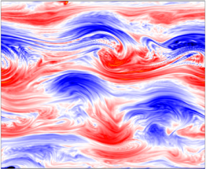
Figure 5. Self-organization of zonal flow (grey level represents to the local value of  $\omega$). (a) Initial condition with finite circulation
  $C_F=0.21$ and impulse
  $C_L=0.11$. (b) Creation of zonal flow observed at
  $t=20$.

Figure 6. The Fourier spectrum of the zonal vorticity  $\omega _z=\mathcal {P}_z \omega$ in the self-organized state (
 $t=20$). The eigenvalue
  $\lambda \sim 5{\rm \pi}$ is dominant.
To make a comparison with the theoretical estimate of zonal enstrophy, we plot  $Z_\lambda$ (the theoretical minimum of zonal enstrophy) and
  $C_E \lambda ^2$ (the theoretical maximum of zonal enstrophy), evaluated for the parameters determined by the given initial condition, in figure 7. As
  $\lambda =5{\rm \pi}$ is the dominant mode (figure 6), we obtain
  $Z_\lambda = 0.69$ and
  $C_E \lambda ^2 = 8.8$. In figure 8, we compare the simulation results and the theoretical estimates, demonstrating that the actual zonal enstrophy
  $Z(\omega )$ stays between the theoretical minimum and maximum; the estimate of the lower bound is reasonably accurate.

Figure 7. The graphs of  $Z_\lambda$ and
  $C_E \lambda ^2$, evaluated for the parameters corresponding to the simulation of figure 5. The points on the curve indicate the eigenvalues.

Figure 8. Evolution of the zonal enstrophy  $Z(\omega )$, and its comparison with the theoretical minimum
  $Z_\lambda$ and the maximum
  $C_E \lambda ^2$ evaluated for the self-organized state
  $\lambda \sim 5{\rm \pi}$. To demonstrate the sensitivity of the minimum value, we also show the theoretical minimum
  $Z_\lambda$ evaluated for
  $\lambda \sim 5{\rm \pi}$,
  $7{\rm \pi}$,
  $9{\rm \pi}$ and
  $11{\rm \pi}$.
5.3. Improved Rhines scale
The forgoing discussion depends on the a posteriori estimate of the eigenvalue  $\lambda$. As discussed in § 4.5, however, we need an a priori estimate of
  $\lambda$ to make the theory useful. While the Rhines scale
  $L_R$ has been proposed to estimate
  $\lambda \sim {\rm \pi}/L_R$, it turns out to be too crude. Here, we propose an improved Rhines scale to make more accurate estimates. Figure 9 compares the dominant scale in the final state obtained by simulation and the Rhines scale for different values of
  $\beta$. It is shown that the dominant scale is approximately 3 times of the Rhines scale.

Figure 9. The comparison between the dominant scale in the self-organized state and the Rhines scale for different values of  $\beta$.
The Rhines scale (4.60) is the length scale  $L_R$ at which the magnitudes of the nonlinear term
  $\{\omega ,\psi \}$ and the linear term
  $\beta \{ y, \psi \}$ become comparable. However, it seems that the function of the nonlinear term, that derives the relaxation of the enstrophy level
  $\lambda$, does not end immediately at
  $L_R$; the numerical experiment shows that the relaxation continues up to
  $\sim 3\times L_R$, where the magnitude of the nonlinear term becomes approximately one eighth of the linear term. Therefore, we propose to use
  $L^*_R = 3 L_R$ for the a priori estimate
  $\lambda = {\rm \pi}/L^*_R$; modifying (4.61), we estimate
 \begin{equation} \lambda \sim \frac{\rm \pi}{3} \sqrt{\frac{\beta}{2\sqrt{2C_E}}}. \end{equation}
6. Conclusion
We have found a discrete set of zonal enstrophy levels that are quantized by the eigenvalue  $\lambda$ measuring the mode number (= system size in the latitude direction/lamination number). As shown in figure 3, a finite circulation
  $C_F$ and/or impulse
  $C_L$ brings about symmetry breaking in the eigenstates (minimizers), inhibiting even mode numbers. In the actual situation, however, the mixed state may include spectra of even mode numbers (see figure 6). By comparing to simulation results, we verified that the theoretical value
  $Z_\lambda$ gives a reasonable estimate of the zonal enstrophy, if we choose the relevant mode number. We note that the enstrophy levels are determined independently of the selection mechanism. Just as the quantum energy level of an orbital electron is lowered by photon emission (see figure 10), the relaxation of the zonal enstrophy level proceeds by the emission of short-scale wavy vorticity. The relaxation process can be viewed as the forward cascade of enstrophy (creation of short-scale wavy vortices) and the simultaneous inverse cascade of the energy spectrum (de-excitation to lower zonal enstrophy states). The energy constraint plays an essential role in selecting the level; the relaxation continues as far as the nonlinear term, measured by the energy, dominates the evolution. The Rhines scale estimates the balance point of the magnitudes of the nonlinear term and the linear Rossby-wave term, but we found that the nonlinear effect continues to work until it becomes approximately one order of magnitude smaller than the linear term, so we propose an improved Rhines scale.

Figure 10. Analogy of quantum energy levels and ‘de-excitation’ by emitting small-scale wavy enstrophy, which parallels the forward cascade of enstrophy.
Comparing Theorems 4.1 and 4.2, we find that the energy constraint  $E(\omega )=C_E$ plays an essential role in creating the discrete zonal enstrophy levels
  $Z_\lambda$. Interestingly, the value of
  $C_E$ does not influence the value of each zonal enstrophy
  $Z_\lambda$, which is determined only by the other constants
  $C_F$ (circulation) and
  $C_L$ (impulse). However, in the absence of the energy constraint, we only have the ‘ground state’
  $\lambda =0$ as given in Theorem 4.1. In the eigenstate of
  $\omega _z$ (belonging to the eigenvalue
  $\lambda$), the zonal enstrophy
  $Z(\omega _z)$ and the zonal energy
  $E(\omega _z)$ are related by
  $Z(\omega _z)=\lambda ^2 E(\omega _z)$. Under the energy constraint (and a fixed
  $\lambda$), therefore,
  $Z(\omega _z)$ may take a smaller value when the wavy component
  $\omega _w$ shares a larger energy
  $E(\omega _w)$. The simultaneous total enstrophy constraint contributes to determining the wavenumber
  $k$ of the wavy component
  $\omega _w$. Without the symmetry breaking constraints by the circulation
  $F(\omega )$ and the impulse
  $L(\omega )$,
  $E(\omega _z)$ can minimize to zero (see figure 1), and then,
  $k\rightarrow \infty$ (independently of the specific value of
  $C_Q$). Finite symmetry breaking by
  $C_F$ and/or
  $C_L$ brings about a non-trivial minimum
  $E(\omega _z)$ (and the corresponding
  $Z(\omega _z)=\lambda ^2 E(\omega _z)$). Then, the partition of the energy to the wavy component is determined as
  $E(\omega _w)=C_E- E(\omega _z)$, and the wavenumber
  $k$ is determined by
  $k^2 E(\omega _w) = C_Q-Z(\omega _z)$. Interestingly, we may not remove the total enstrophy constraint from the variational principle, in order to retain a finite wavy component as the complementary to the zonal component, while its role is limited to characterizing only the wavy component. This unusual phenomenon in the variational principle is caused by the non-coerciveness of the target functional
  $Z(\omega )$ with respect to the norm
  $\|\omega \|$.
Acknowledgements
The authors thank Y. Kawazura for his support in the simulation study. The suggestions of the editor for improving the manuscript are appreciated.
Funding
This work was supported by JSPS KAKENHI (grant number 17H01177).
Declaration of interests
The authors report no conflict of interest.
Appendix A. The ABC of the variational principle
To see the mathematical non-triviality of the variational principle for the zonal enstrophy, we review the standard relation between the target functional and constraint.
A.1. Target functional and constraint
We start with a textbook example. The isoperimetric problem is to (i) maximize the surface area  $S$ with a constraint on the periphery length
  $L$, or (ii) minimize the peripheral length
  $L$ with a constraint on the surface area
  $S$. Both problems have the same solution, i.e. a circular disk or its periphery. Notice that reversing the target and constraint in each setting results in an ill-posed problem; one can make
  $L$ infinitely long without changing
  $S$, or one can make
  $S$ infinitely small without changing
  $L$. Let us concentrate on minimization problems. For a variational principle to be well posed, the target (
 $L$) must be ‘fragile’ and the constraint (
 $S$) must be robust. Here, the fragility speaks of the sensitivity to small-scale perturbations. Suppose that we make pleats on a periphery; then
  $L$ is increased, but
  $S$ is not necessarily changed. In analytical formalism, a fragile functional includes a larger number of differentiations – derivatives are sensitive to small-scale perturbations. In the forgoing example, we may formally write
 \begin{equation} S = \int_{\mathbb{R}^2} \mathbb{I}_M \mathrm{d}^2 x, \quad L= \int_{\mathbb{R}^2} |\boldsymbol{\nabla} \mathbb{I}_M| \mathrm{d}^2 x, \quad \mathbb{I}_M(\boldsymbol{x}) = \left\{ \begin{array}{@{}ll} 1 & \mathrm{if}\ \boldsymbol{x} \in M\\ 0 & \mathrm{if}\ \boldsymbol{x} \notin M, \end{array} \right. \end{equation}
where  $M$ is a simply connected domain
  $\subset \mathbb {R}^2$ that should be optimized to minimize
  $L$ for some given value of
  $S$. Including
  $\boldsymbol {\nabla }$ in the integrand,
  $L$ is fragile.
A.2. Coerciveness and continuity
To make the argument more precise, we introduce the notion of coercive functionals; cf. Yoshida & Mahajan (Reference Yoshida and Mahajan2002); Lions & Magenes (Reference Lions and Magenes2012). Let  $u$ be a real-valued function (state vector) belonging to a function space (phase space)
  $V$, which is a Banach space with a norm
  $\|u \|$. A real-valued functional
  $G(u)$ is said to be coercive if
 \begin{equation} \| u \|^2 \leq c\, G(u), \end{equation}
where  $c$ is some positive constant. On the other hand, a real-valued functional
  $H(u)$ is continuous if
 \begin{equation} | H(u+\delta) - H(u) | \rightarrow 0 \quad (\| \delta \| \rightarrow 0). \end{equation}
We can formulate a well-posed minimization problem with a coercive target functional  $G(u)$ and a continuous constraining functional
  $H(u)$ (we may also consider multiple constraints with continuous functionals).
To see how the coerciveness and continuity influence variational principles, let us consider an example with two functionals
 \begin{equation} {G}(u) = \int_M |\boldsymbol{\nabla} u(\boldsymbol{x})|^2 \,\mathrm{d}^n x, \quad {H}(u) = \int_M |u(\boldsymbol{x})|^2 \mathrm{d}^n x , \end{equation}
where  $u$ is a scalar function defined in a smoothly bounded open set
  $M\subset \mathbb {R}^n$. We assume that
  $u=0$ on the boundary
  $\partial M$. Notice that
  ${H}(u)^{1/2}$ is the
  $L^2$ norm
  $\| u \|$. Therefore,
  $H(u)$ is a continuous functional on the function space
  $V=L^2(M)$. By the Poincaré inequality, we have
 \begin{equation} \| u \|^2 \leq c \| \boldsymbol{\nabla} u \|^2 = c G(u), \end{equation}
with a positive constant  $c$. Therefore,
  $G(u)$ is a coercive functional.
First, we seek a minimizer of  ${G}(u)$ with the constraint
  ${H}(u) =1$. This is a well-posed problem. The minimizer is found by the variational principle
 \begin{equation} \delta [{G}(u) - \lambda{H}(u)] =0, \end{equation}
where  $\lambda$ is a Lagrange multiplier. The Euler–Lagrange equation
 \begin{equation} -\varDelta u = \lambda u, \end{equation}
together with the above-mentioned boundary condition, constitute an eigenvalue problem. We can easily show that every eigenvalue  $\lambda$ is positive. Let
  $\lambda _j$ be an eigenvalue and
  $\varphi _j$ be the corresponding normalized eigenfunction (
 $\| \varphi _j\|^2 =1$). Setting
  $u = a\varphi _j$ and demanding
  ${H}(u)=1$, we obtain
  $a=1$ and
  ${G}(u) = \lambda _j$. The smallest
  $\lambda _j$, then, yields the minimum
  ${G}(u)$.
The reverse problem of finding a minimizer of  ${H}(u)$ with the restriction
  ${G}(u) =1$ is ill posed, because the constraint is posed by a functional
  $G(u)$ that is not continuous in the topology of
  $L^2(M)$. Let us elucidate the pathology. The variational principle
  $\delta [{H}(u) - \mu {G}(u)] =0$ (
 $\mu$ is a Lagrange multiplier) yields the Euler–Lagrange equation
  $-\varDelta u = \mu ^{-1} u$. Let
  $\mu ^{-1} = \lambda _j$ (an eigenvalue of
  $-\varDelta$), and
  $u=a \varphi _j$. The condition
  ${G}(u) =1$ yields
  $a=\lambda _j^{-1/2}$, and
  ${H}(u) = 1/\lambda _j$. Hence, the minimum of
  ${H}(u)$ is achieved by the largest eigenvalue that is unbounded, viz.,
  $\mathrm {inf} {H}(u) = 0$ and the minimizer
  $\lim _{\lambda _j \rightarrow \infty } \lambda _j^{-1/2} \varphi _j = 0$ is nothing but the minimizer of
  ${H}(u)$ without any restriction. The constraint
  ${G}(u) =1$ plays no role in this minimization problem.
A.3. Non-coercive target functional
Let us modify the target functional of (A6) to a non-coercive functional. Let  $V_k = \mathrm {span}\,\{ \varphi _1, \ldots , \varphi _k \}$, which is a closed (finite-dimensional) subspace of
  $V=L^2(M)$. We denote the orthogonal complement by
  $V'$, i.e. we decompose
  $V= V_k \oplus V'$. Let
  $\mathcal {P}$ be the orthogonal projector
  $V \rightarrow V'$. Consider
 \begin{equation} G' (u) = \| \boldsymbol{\nabla} (\mathcal{P} u)\|^2 = \int_M (-\varDelta \mathcal{P} u) (\mathcal{P} u)\,\mathrm{d}^n x = \sum_{j>k}^\infty \lambda_j (u, \varphi_j)^2 , \end{equation}
where  $(f,g) = \int _M f(\boldsymbol {x})\,g(\boldsymbol {x}) \,\mathrm {d}^n x$ is the inner product of
  $L^2(M)$. Evidently,
  $G'(u)$ is not coercive. The modified variational principle
 \begin{equation} \delta [{G}' (u) - \lambda{H}(u)] =0 \end{equation}
yields the Euler–Lagrange equation that reads, after expanding with eigenfunctions,
 \begin{equation} \lambda'_j (u,\varphi_j) = \lambda (u,\varphi_j) \quad (j=1,2,\ldots), \end{equation}
where the ‘modified eigenvalues’ are
 \begin{equation} \lambda'_j = \left\{ \begin{array}{@{}ll} 0, & (j=1,\ldots, k),\\ \lambda_j , & (j> k).\end{array} \right. \end{equation}
The minimizer of  $G'(u)$ is a solution of (A10) such that
  $\lambda =0$ and
 \begin{equation} u = \sum_{j=1}^k a_j \varphi_j, \end{equation}
where constants  $a_1,\ldots ,a_k$ can be arbitrarily chosen provided that
  $\sum _{j=1}^k |a_j|^2 = 1$ in order to satisfy the constraint
  $H(u)=1$. We obtain
  $\mathrm {min}\,G' = 0$, but the minimizer is not a unique function.
This prototypical example elucidates the essence of the pathology created in a variational principle with non-coercive target functional. We encounter a similar non-uniqueness (degeneracy) problem in § 4.1. Interestingly, however, the energy constraint brings about a dramatical change in the mathematical structure, and removes the degeneracy; § 4.3.


 Open access