I. INTRODUCTION
The author has proposed a deconvolutional treatment on powder diffraction data collected with a measurement system based on the Bragg-Brentano geometry (Ida and Toraya, Reference Ida and Toraya2002; Ida et al., Reference Ida, Ono, Hattan, Yoshida, Takatsu and Nomura2018). The treatment automatically corrects the peak shift and asymmetric deformation of the peak shape caused by the instrumental aberrations in the observed data, provided that the assumed instrumental aberration functions and the instrumental parameters are correct. Since the treatment keeps the effects of the even-order cumulants of the aberration function unchanged, the integrated intensity, peak width, and sharpness of the peak are not changed by the treatment, while it is also easy to introduce automatic intensity correction in the treatment at the same time (Ida, Reference Ida2020a).
The deconvolution is usually recognized as the inverse Fourier transform of the quotient of the Fourier transform of the observed data by the Fourier transform of the instrumental function (e.g., Press et al., Reference Press, Teukolsky, Vetterling and Flannery2007). In this article, what this author intends to mean by the deconvolutional treatment is the insertion of multiplication by the complex absolute values ![]() $\vert {{\cal F}( k ) } \vert$ of the Fourier transform
$\vert {{\cal F}( k ) } \vert$ of the Fourier transform ![]() ${\cal F}( k )$ of the instrumental function f(x) into the usual deconvolution process. The additional computing cost is negligible. The treatment is equivalent to commutative double operations, one is the deconvolution with the instrumental function f(x), and another is the convolution with the symmetrized instrumental function, the author would like to express by the symbol |f|(x).
${\cal F}( k )$ of the instrumental function f(x) into the usual deconvolution process. The additional computing cost is negligible. The treatment is equivalent to commutative double operations, one is the deconvolution with the instrumental function f(x), and another is the convolution with the symmetrized instrumental function, the author would like to express by the symbol |f|(x).
The symmetrized instrumental function |f|(x) in the above context is defined as the inverse Fourier transform of ![]() $\vert {{\cal F}( k ) } \vert$. It may be easier to find how the cumulants are changed on the deconvolutional treatment when the following mathematical relations are recognized.
$\vert {{\cal F}( k ) } \vert$. It may be easier to find how the cumulants are changed on the deconvolutional treatment when the following mathematical relations are recognized.
The Fourier transform of convolution is equivalent to the product of the Fourier transforms of the component functions, which is known as the convolution theorem (e.g., Press et al., Reference Press, Teukolsky, Vetterling and Flannery2007).
Apart from the Fourier transform, a cumulant of convolution is equivalent with the sum of the cumulants of component functions at any order, which may be called the additivity of cumulants on convolution. The relation is immediately derived from the definition of the jth order cumulant of a function f(x), given by
and a symmetric expression of the convolution f(x)*g(x), given by
where δ(x) is the Dirac delta function.
The autocorrelation of a function f(x), the author would like to express by the symbol |f|2(x), is equivalent to the convolution of f(x) and f( − x). The function |f|2(x) is symmetric in the sense expressed by the equation |f|2( − x) = |f|2(x). The autocorrelation function |f|2(x) has twice even-order cumulants and zero odd-order cumulants, as directly derived from the additivity of cumulants. On the other hand, Fourier transform of the autocorrelation is equivalent to the product of the Fourier transform ![]() ${\cal F}( k )$ of the function f(x) and its complex conjugate
${\cal F}( k )$ of the function f(x) and its complex conjugate ![]() ${\cal F}^\ast ( k )$, as expressed by
${\cal F}^\ast ( k )$, as expressed by ![]() $\vert {{\cal F}( k ) } \vert ^2\equiv {\cal F}( k ) {\cal F}^\ast ( k ).\;\;$The symmetrized function |f|(x) is defined as the inverse Fourier transform of
$\vert {{\cal F}( k ) } \vert ^2\equiv {\cal F}( k ) {\cal F}^\ast ( k ).\;\;$The symmetrized function |f|(x) is defined as the inverse Fourier transform of ![]() $\vert {{\cal F}( k ) } \vert = \sqrt {{\cal F}( k ) {\cal F}^\ast ( k ) }$. The autocorrelation function of the symmetrized function |f|(x) is clearly identical to |f|2(x). The even-order cumulants of the function |f|(x) should exactly be half of those of autocorrelation function |f|2(x), and equal to those of the function f(x), while all the odd-order cumulants of |f|(x) are zero.
$\vert {{\cal F}( k ) } \vert = \sqrt {{\cal F}( k ) {\cal F}^\ast ( k ) }$. The autocorrelation function of the symmetrized function |f|(x) is clearly identical to |f|2(x). The even-order cumulants of the function |f|(x) should exactly be half of those of autocorrelation function |f|2(x), and equal to those of the function f(x), while all the odd-order cumulants of |f|(x) are zero.
The deconvolutional treatment exactly cancels the instrumental effects expressed by the odd-order cumulants, but keeps the effects expressed by the even-order cumulants unchanged. In other words, the deconvolution with f(x) removes all the cumulants of f(x), and the convolution with |f|(x) selectively recovers the effects related to the even-order cumulants of the function f(x).
It may also be noted that the addition of the function f( − x) to the function f(x) also cancels the odd-order cumulants and make the even-order power averages exactly twice at any order, but do not make the even-order cumulants twice at the fourth and higher orders.
It is much easier to calculate the cumulants than to derive a formula of the instrumental aberration function (Ida, Reference Ida2020a). As the cumulants of convolution are equivalent to the sum of the cumulants of the component functions at any order, it is naturally expected that the use of cumulants will simplify modeling the experimentally observed data, usually considered as multiple convolutions with instrumental effects. What we should calculate for the multiple convolutions of instrumental functions will not be the multiple integrations, but the addition, when we use the cumulants of the instrumental functions.
However, it is well known that the first- and higher-order cumulants of the Lorentzian function cannot be defined. The cumulants of the first and higher orders can neither be defined for the Voigt, pseudo-Voigt, and Pearson VII functions, while they are still often used for curve-fitting analysis of observed spectroscopic or diffraction peak profiles, even though the use of the Voigt function is justified only for the Mössbauer spectroscopy, to the author's knowledge.
In contrast to the Lorentzian and related functions, any order of cumulants of an instrumental function can be defined, in general. All the parameters to specify the deviation are limited within a finite range, because they are restricted by the finite geometric dimensions of the instrument. When the domain of a normalized function is bounded, any order of cumulants can be defined.
The evaluation of higher-order cumulants generally needs more computation time and higher accuracy of numerical system to be used for calculation, while higher-order cumulants will become less significant in the statistical or practical point of view. Particular statistical analysis based on experimental data of 5000 sample values has shown 2.7–2.9 significant digits for the estimated first-order cumulant (average), 1.2–1.6 significant digits for the second-order cumulant (variance), and 0.7–0.9 significant digits for the third-order cumulant, for example (Ida, Reference Ida2011).
In this study, the author limits the order of cumulants up to the fourth and focuses on the construction of a series of symmetric functions uniquely determined by the second- and fourth-order cumulants. The kurtosis k, defined by the ratio of the fourth-order cumulant to the square of the second-order cumulant, is treated as the variable parameter to specify the sharpness of the peak shape, while the second-order cumulant, or the standard deviation defined as the square root of the second-order cumulant, is directly connected to the width of the function.
It will be favorable, in the practical point of view, that the rectangular function, which has the most flattened or collapsed shape as a unimodal function, is included in the system. A knife-edge slit is one of the commonly used optical elements. If the effect of finite open width of a knife-edge slit is dominant, the instrumental function should really have a rectangular shape. The kurtosis of the rectangular shape is k = −6/5 = −1.2.
In the range of the kurtosis from k = −1.2 to k = 0, the product of the rectangular function and the Gaussian function, which may be called the truncated Gaussian function, is used in the system. If the truncation width is narrower than the standard deviation of the Gaussian, the shape approaches to rectangular, and if the truncation width is wider enough, it becomes equivalent to the Gaussian function. The choice of the convolution of the Gaussian and rectangular functions, which is not difficult to be calculated, may appear more natural, but it will introduce complexity to formulate or calculate the inverse primitive function, which will be required for the application of an efficient algorithm (Ida, Reference Ida1998) to evaluate the convolution with the Lorentzian function.
In the range of the kurtosis from k = 0 to k = 3, the product of the Gaussian function and the symmetric (truncated) exponential function with the kurtosis of k = 3 is used. The function has such shape as the center part of the Gaussian function is trimmed away, and remained tail parts of the Gaussian function are shifted to and connected at the origin. The author would like to call the function as the sheared Gaussian function to avoid confusion. It may also be noted that the function is identical to the Fourier transform of the Voigt function. Not the convolution, but the product is chosen, for the convenience to apply an efficient algorithm, similarly to the truncated Gaussian function.
In the range of the kurtosis k ≥ 3, a symmetric Rosin-Rammler-type function is used in the current system. The choice of symmetric (reflected) density function of the gamma distribution function may appear more natural, but it is often difficult to utilize the numerical library for the evaluation of the inverse primitive function. The formulas for the primitive and inverse primitive functions of the Rosin-Rammler-type function are quite simple. The asymmetric formula of the function has first been used for the analysis of particle size distribution of powder samples (Rosin and Rammler, Reference Rosin and Rammler1933). The same distribution is also called the Weibull distribution in the field of mechanical engineering (Weibull, Reference Weibull1951). It seems that there is no theoretical base, but Rosin-Rammler or Weibull distribution is convenient for calculation, anyway.
A practical method to calculate the convolution of the symmetric function with the Lorentzian function is briefly described in Section III. It should be emphasized that the Voigt function will become a special case for k = 0 when the current system is expanded by the convolution with the Lorentzian function.
The results of the application of the mathematical system to the analysis of observed powder diffraction data are demonstrated and discussed in Section IV.
II. SYMMETRIC FUNCTIONS
A. Truncated Gaussian function
A normalized formula of the truncated Gaussian function with a width (scale) parameter γ and a shape parameter a is given by
 $$f_{{\rm TG}}( {x; \;\gamma , \;a} ) = \left\{{\matrix{ {\displaystyle{1 \over {\sqrt {\rm \pi } \gamma {\rm erf}( a ) }}\exp \left({-\displaystyle{{x^2} \over {\gamma^2}}} \right)} \hfill & {[ {\vert x \vert < \gamma a} ] } \hfill \cr 0 \hfill & {[ {{\rm elsewhere}} ] } \hfill \cr } } \right.\;, \;$$
where erf(x) is the error function defined by
The error function erf(x) is provided as a callable function in most of numerical libraries for computing.
The second power average of the function f TG(x;γ, a), which is equivalent to the second-order cumulant (variance) in case of a symmetric function, is given by
and the fourth power average is given by
The fourth-order cumulant ![]() $\langle \kappa_4\rangle_{\rm TG}(\gamma, a)$ of the symmetric function is given by
$\langle \kappa_4\rangle_{\rm TG}(\gamma, a)$ of the symmetric function is given by
Figure 1 plots the values of the (excess) kurtosis ![]() $k_{{\rm TG}}( a ) = \langle x^4\rangle_{{\rm TG}} ( {\gamma , \;a} ) /[ {\langle x^2 \rangle_{{\rm TG}} ( {\gamma , \;a} ) } ] ^2-3$ versus the values of the complementary error function defined by erfc(a) ≡ 1 − erf(a). The complementary error function erfc(x) is also included in usual libraries for computation, because the error function erf(x) rapidly loses significant digits for large values of x, while the complementary error function erfc(x) keeps more significant digits for large x in the standard numerical system for floating point numbers defined as IEEE 754 for computation. Both the inverse functions, erf−1(x) and erfc−1(x), are provided as callable functions, in usual numerical libraries, even if the precision of the values of the function may not be certified.
$k_{{\rm TG}}( a ) = \langle x^4\rangle_{{\rm TG}} ( {\gamma , \;a} ) /[ {\langle x^2 \rangle_{{\rm TG}} ( {\gamma , \;a} ) } ] ^2-3$ versus the values of the complementary error function defined by erfc(a) ≡ 1 − erf(a). The complementary error function erfc(x) is also included in usual libraries for computation, because the error function erf(x) rapidly loses significant digits for large values of x, while the complementary error function erfc(x) keeps more significant digits for large x in the standard numerical system for floating point numbers defined as IEEE 754 for computation. Both the inverse functions, erf−1(x) and erfc−1(x), are provided as callable functions, in usual numerical libraries, even if the precision of the values of the function may not be certified.
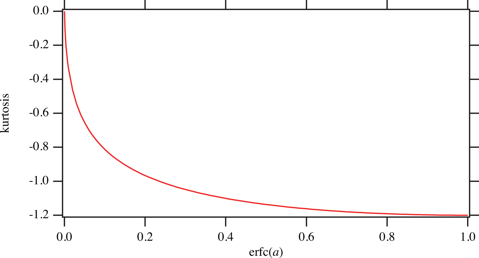
Figure 1. Kurtosis of the truncated Gaussian function versus the values of complementary error function erfc(a) of the shape parameter a.
Since the function k TG(a) is a monotonous one-variable function of erfc(a), as can be seen in Figure 1, it is not difficult to solve the equation, k = k TG(a), by a numerical method, a bisection method or a Newton method, for example (e.g. Press et al., Reference Press, Teukolsky, Vetterling and Flannery2007), or a method referring to a numerical table, as conventionally used in the field of crystallography, as known as “International Tables for Crystallography”. Table I lists the values of erfc(a) and the shape parameter a for given values of kurtosis k.
TABLE I. Values of the complementary error function erfc(a) and shape parameter a of the truncated Gaussian function for given values of kurtosis, k.

When the value of kurtosis k is indicated, the shape parameter a of the truncated Gaussian function is uniquely determined, and the width parameter γ is calculated from the standard deviation σ and the value of a by solving Eq. (5), that is,
 $$\gamma = \sigma \left[{\displaystyle{1 \over 2}-\displaystyle{{a\exp ( {-a^2} ) } \over {\sqrt {\rm \pi } {\rm \;erf}( a ) }}} \right]^{{-}1/2}\;.$$
The formulas for the cases of k = −1.2 and k = 0 are exceptional. The function approaches to the rectangular function with the formula:
 $$f_{\rm R}( {x; \;\sigma } ) = \left\{{\matrix{ {\displaystyle{1 \over {2\sqrt 3 \sigma }}} \hfill & {\left[{\vert x \vert < \sqrt 3 \sigma } \right]} \hfill \cr 0 \hfill & {[ {{\rm elsewhere}} ] } \hfill \cr } } \right.\;, \;$$
at the k → −1.2 limit and to the Gaussian function with the formula:
at the k → 0 limit, for the standard deviation of σ.
Figure 2 shows a series of the truncated Gaussian functions with the common value of standard deviation σ = 1.
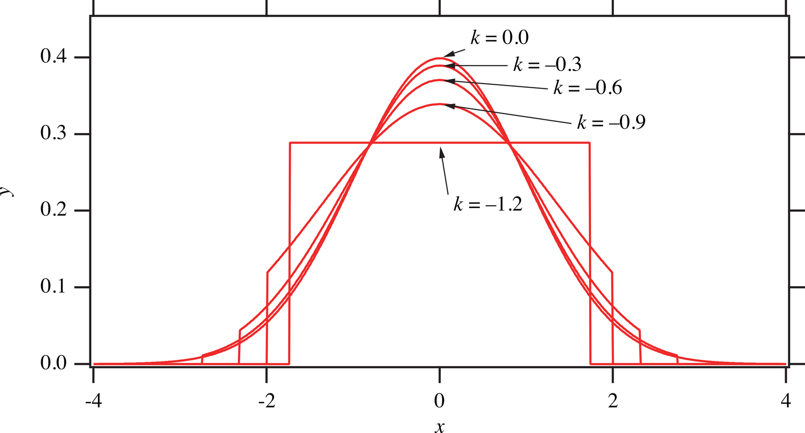
Figure 2. Series of truncated Gaussian functions with the standard deviation of unity.
The primitive function F TG(x;γ, a) of the truncated Gaussian function f TG(x;γ, a) is given by
and the inverse function ![]() $F_{{\rm TG}}^{{-}1} ( {y; \;\gamma , \;a} )$ of the primitive function F TG(x;γ, a) is given by
$F_{{\rm TG}}^{{-}1} ( {y; \;\gamma , \;a} )$ of the primitive function F TG(x;γ, a) is given by
The inverse function of the error function, erf−1(x), is provided as a callable function in a usual computing system, even if the accuracy of the values of the function may not be certified.
B. Sheared Gaussian function
A normalized formula of the sheared Gaussian function for a width parameter s and a shape parameter b is given by
where erfcx(x) is the scaled complementary error function defined by erfcx(x) ≡ exp(x 2)erfc(x). It is not difficult to evaluate the inverse function erfcx−1(x) by a numerical method, a Newton method for example, even if it may be difficult to use a numerical library including the inverse function erfcx−1(x).
The second power average of the function f SG(x;s, b) is given by
and the fourth power average is given by
Figure 3 plots the values of the kurtosis ![]() $k_{{\rm SG}}( b ) = \langle x^4 \rangle_{{\rm SG}} ( {s, \;b} ) /[ {\langle x^2 \rangle_{{\rm SG}} ( {s, \;b} ) } ] ^2-3$ versus the values of the scaled complementary error function erfcx(b) of the shape parameter b.
$k_{{\rm SG}}( b ) = \langle x^4 \rangle_{{\rm SG}} ( {s, \;b} ) /[ {\langle x^2 \rangle_{{\rm SG}} ( {s, \;b} ) } ] ^2-3$ versus the values of the scaled complementary error function erfcx(b) of the shape parameter b.
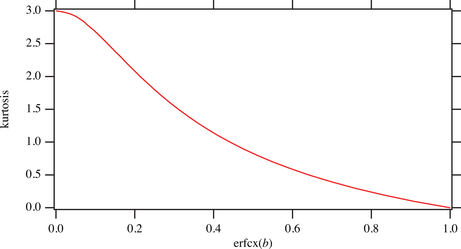
Figure 3. Kurtosis of the sheared Gaussian function versus the values of scaled complementary error function erfcx(b) of the shape parameter b.
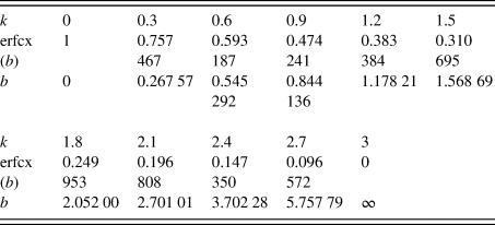
Table II lists the values of erfcx(b) and the shape parameter b of the sheared Gaussian function for given values of kurtosis k.
TABLE II. Values of the scaled complementary error function erfcx(b) and shape parameter b of the sheared Gaussian function for given kurtosis, k.
When the value of kurtosis k is indicated, the shape parameter b of the sheared Gaussian function is uniquely determined, and the width parameter s is calculated from the standard deviation σ and the value of b by solving Eq. (14), that is,
The case of k = 0 is not exceptional in the sheared Gaussian function, and the function expressed by Eq. (13) naturally reduces to the Gaussian function given by Eq. (10) for k = 0. The case of k → 3 is exceptional, and it approaches to the symmetric truncated exponential function f STE(x;σ) given by
Figure 4 shows a series of the sheared Gaussian functions with the standard deviation σ = 1.
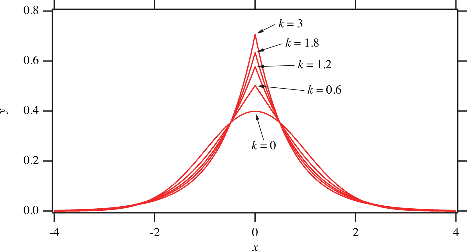
Figure 4. Series of sheared Gaussian functions with the standard deviation of unity.
The primitive function F SG(x;s, b) of the truncated Gaussian function f SG(x;s, b) is given by
 $${\rm sign}( x ) \equiv \left\{{\matrix{ 1 & {[ {x > 0} ] } \cr 0 & {[ {x = 0} ] } \cr {-1} & {[ {x < 0} ] } \cr } } \right., \;$$
and the inverse function ![]() $F_{{\rm SG}}^{{-}1} ( {y; \;s, \;b} )$ of the primitive function F SG(x;s, b) is given by
$F_{{\rm SG}}^{{-}1} ( {y; \;s, \;b} )$ of the primitive function F SG(x;s, b) is given by
C. Symmetric Rosin-Rammler-type function
A normalized formula of the symmetric Rosin-Rammler-type function f SRR(x;g, h) with a width parameter g and a shape parameter h is given by
 $$f_{{\rm SRR}}( {x; \;g, \;h} ) = \displaystyle{h \over {2g}}\left({\displaystyle{{\vert x \vert } \over g}} \right)^{h-1}{\rm exp}\left[{-{\left({\displaystyle{{\vert x \vert } \over g}} \right)}^h} \right]{\rm \;}, \;$$
and the shape parameter h is restricted in the range h ≤ 1, in the current system. The value of the function diverges to infinity at the origin for the values h < 1.
The second power average of the function f SRR(x;g, h) is given by
where Γ(x) is the complete gamma function, defined by
The complete gamma function Γ(x), or the logarithm of the function ln Γ(x), is provided as callable functions in a usual computing system.
The fourth power average of the symmetric Rosin-Rammler-type function is given by
Figure 5 plots the values of kurtosis k SRR(h) = ![]() $\langle x^4 \rangle_{{\rm SRR}} ( {g, \;h} ) /[ {\langle x^2 \rangle_{{\rm SRR}} ( {g, \;h} ) } ] ^2-3$ versus the value of the shape parameter h.
$\langle x^4 \rangle_{{\rm SRR}} ( {g, \;h} ) /[ {\langle x^2 \rangle_{{\rm SRR}} ( {g, \;h} ) } ] ^2-3$ versus the value of the shape parameter h.
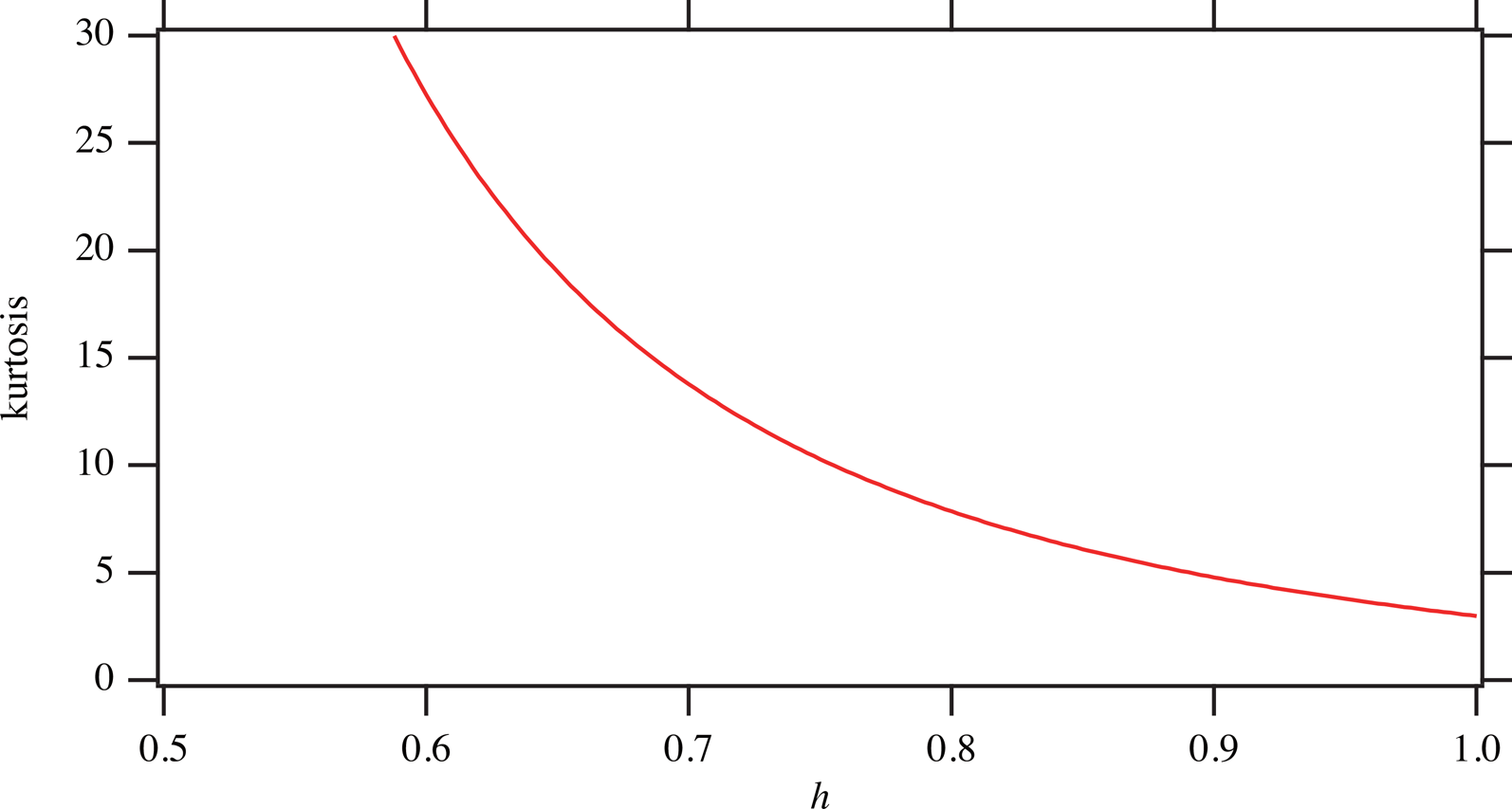
Figure 5. Kurtosis of the symmetric Rosin-Rammler-type function depending on the shape parameter h.
Table III lists the values of the shape parameter h of the symmetric Rosin-Rammler-type function for given values of kurtosis k.
TABLE III. Values of the shape parameter h of the symmetric Rosin-Rammler function for given values of kurtosis, k

The shape parameter h of the symmetric Rosin-Rammler-type function is uniquely determined by the indicated value of kurtosis k, and the width parameter g is calculated from the standard deviation σ and the value of h by solving Eq. (22), that is,
The formula for the case of k = 3 coincides with the symmetric truncated exponential function given by Eq. (17).
Figure 6 shows a series of symmetric Rosin-Rammler-type functions with the standard deviation of σ = 1.
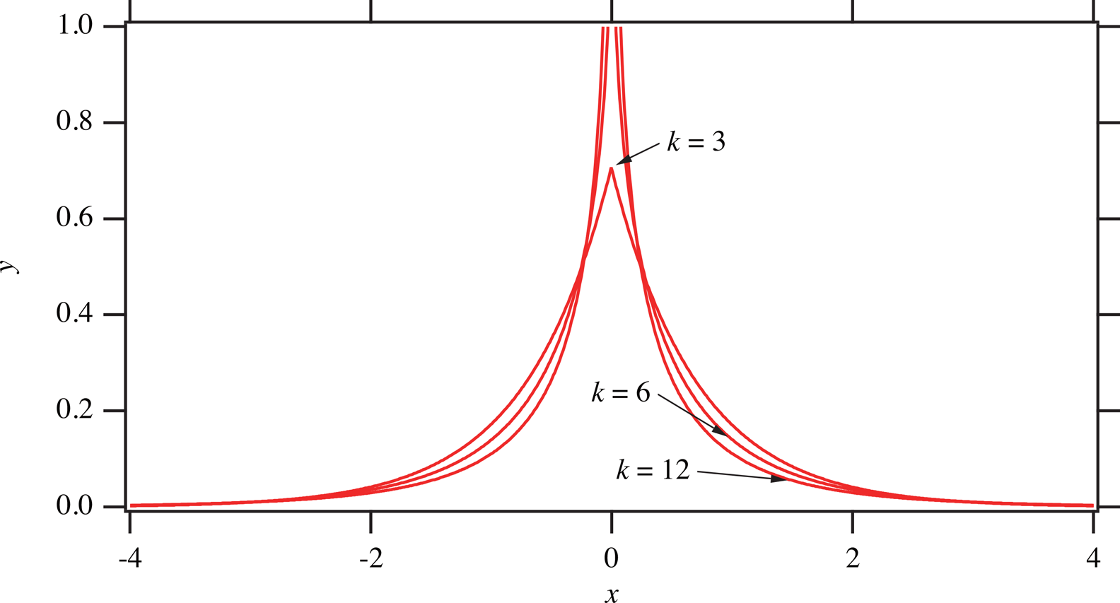
Figure 6. Series of symmetric Rosin-Rammler-type functions with the standard deviation of unity.
The primitive function F SRR(x;g, h) of the symmetric Rosin-Rammler-type functions is given by
 $$F_{{\rm SRR}}( {x; \;g, \;h} ) = \displaystyle{{{\rm sign}( x ) } \over 2}\left\{{1-\exp \left[{-{\left({\displaystyle{{\vert x \vert } \over g}} \right)}^h} \right]} \right\}{\rm \;}.$$
and the primitive function is given by
III. CONVOLUTIONS WITH LORENTZIAN FUNCTION
A. Efficient algorithm for evaluating convolution
The values of the convolution of a Lorentzian function f L(x;w) with the half width at half maximum (HWHM) of w are calculated by
The primitive and inverse primitive functions of f L(x;w) are given by
The values of the convolution of the Lorentzian function f L(x;w) with one of the symmetric functions f X(x;α, β) are commonly calculated by the following formulas (Ida, Reference Ida1998),
 $$f_{{\rm L\ast }X}( {x; \;w, \;\alpha , \;\beta } ) = ( {\xi_{{\rm max}}-\xi_{{\rm min}}} ) \;g_X( {x; \;\alpha , \;\beta } ) \mathop \sum \limits_{\,j = 0}^{N-1} \displaystyle{{W_j\;f_{\rm L}( {y_j; \;w} ) } \over {\,f_{\rm L}( {\eta_j; \;w} ) }}, \;$$
 $$g_X( {x; \;\alpha , \;\beta } ) = \left\{{\matrix{ {\displaystyle{{F_X( {\varepsilon ; \;\alpha , \;\beta } ) } \over \varepsilon }} & {[ {\vert x \vert < \varepsilon } ] } \cr {\displaystyle{{F_X( {x; \;\alpha , \;\beta } ) } \over x}} & {[ {\vert x \vert \ge \varepsilon } ] } \cr } } \right., \;$$
for relative locations and weights, {X j} and {W j}, of a numerical integral. The Gauss-Legendre quadrature (e.g., Press et al., Reference Press, Teukolsky, Vetterling and Flannery2007) can be used, for example, but a mid-point method for numerical integration, which is expressed by the equations,
is also recommendable for simplicity. A small value ɛ, 10−6 for example, is introduced in Eq. (34) to avoid an exceptional behavior of the symmetric Rosin-Rammler-type function at the origin.
B. Application to the analysis of experimental data
The author has shown the equations to calculate the first to fourth cumulants of instrumental aberration functions, including axial-divergence, flat-specimen, and sample-transparency aberrations (Ida, Reference Ida2020b). The total values of cumulants for a typical powder diffraction measurement condition, including the effects of the finite size of the source X-ray and the receiving slit width, have also been demonstrated as a function of the apparent diffraction angle 2Θ.
Table IV lists the values of the standard deviation σ, reduced fourth cumulant ![]() $\kappa _4^{( {1/4} ) }$ and kurtosis k of the total instrumental functions evaluated from the instrumental parameters, and the assumed Lorentzian HWHM w for three diffraction peaks of a Si powder (NIST SRM640d) specimen, where the reduced fourth cumulant
$\kappa _4^{( {1/4} ) }$ and kurtosis k of the total instrumental functions evaluated from the instrumental parameters, and the assumed Lorentzian HWHM w for three diffraction peaks of a Si powder (NIST SRM640d) specimen, where the reduced fourth cumulant ![]() $\kappa _4^{( {1/4} ) }$ is defined by
$\kappa _4^{( {1/4} ) }$ is defined by
TABLE IV. Values of standard deviation σ, reduced fourth cumulant ![]() $\kappa _4^{( {1/4} ) },$ and kurtosis k of the total instrumental functions, and the assumed Lorentzian HWHM w expected for three diffraction peaks of Si, 111, 422, and 533
$\kappa _4^{( {1/4} ) },$ and kurtosis k of the total instrumental functions, and the assumed Lorentzian HWHM w expected for three diffraction peaks of Si, 111, 422, and 533

Figures 7, 8, and 9 compare (a) the observed, deconvolutionally treated (symmetrized) intensity data and (b) the peak profile calculated as the convolution of the Lorentzian and symmetric function determined by the standard deviation σ and the kurtosis k expected from geometrical parameters of the instrument.
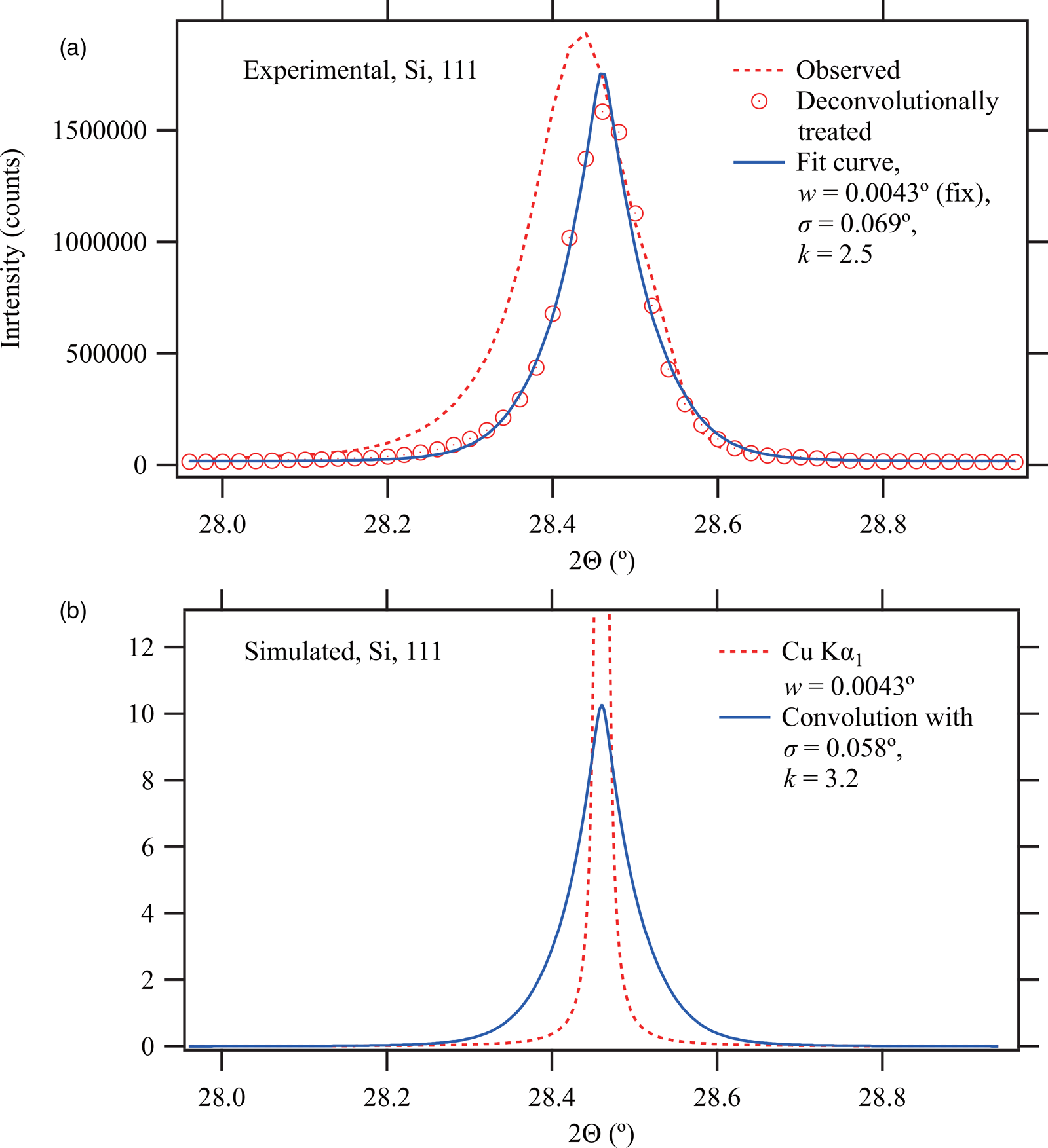
Figure 7. Comparison of (a) experimental (observed and deconvolutionally treated) data and (b) simulated profile predicted from geometrical parameters for Si 111 reflection.
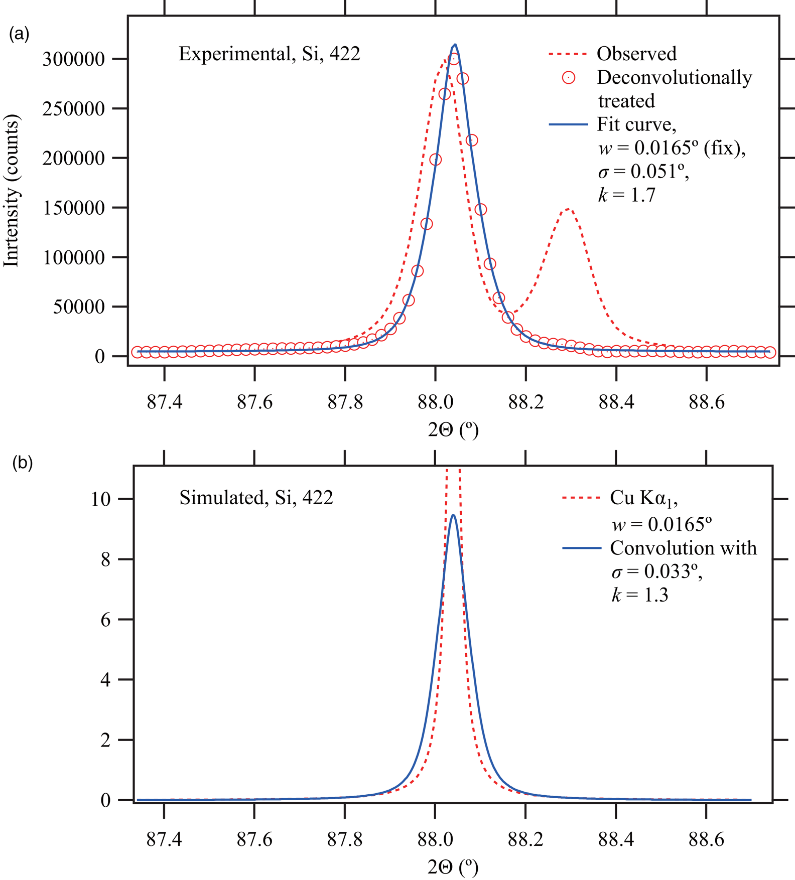
Figure 8. Comparison of (a) experimental and (b) simulated profiles for Si 422 reflection.
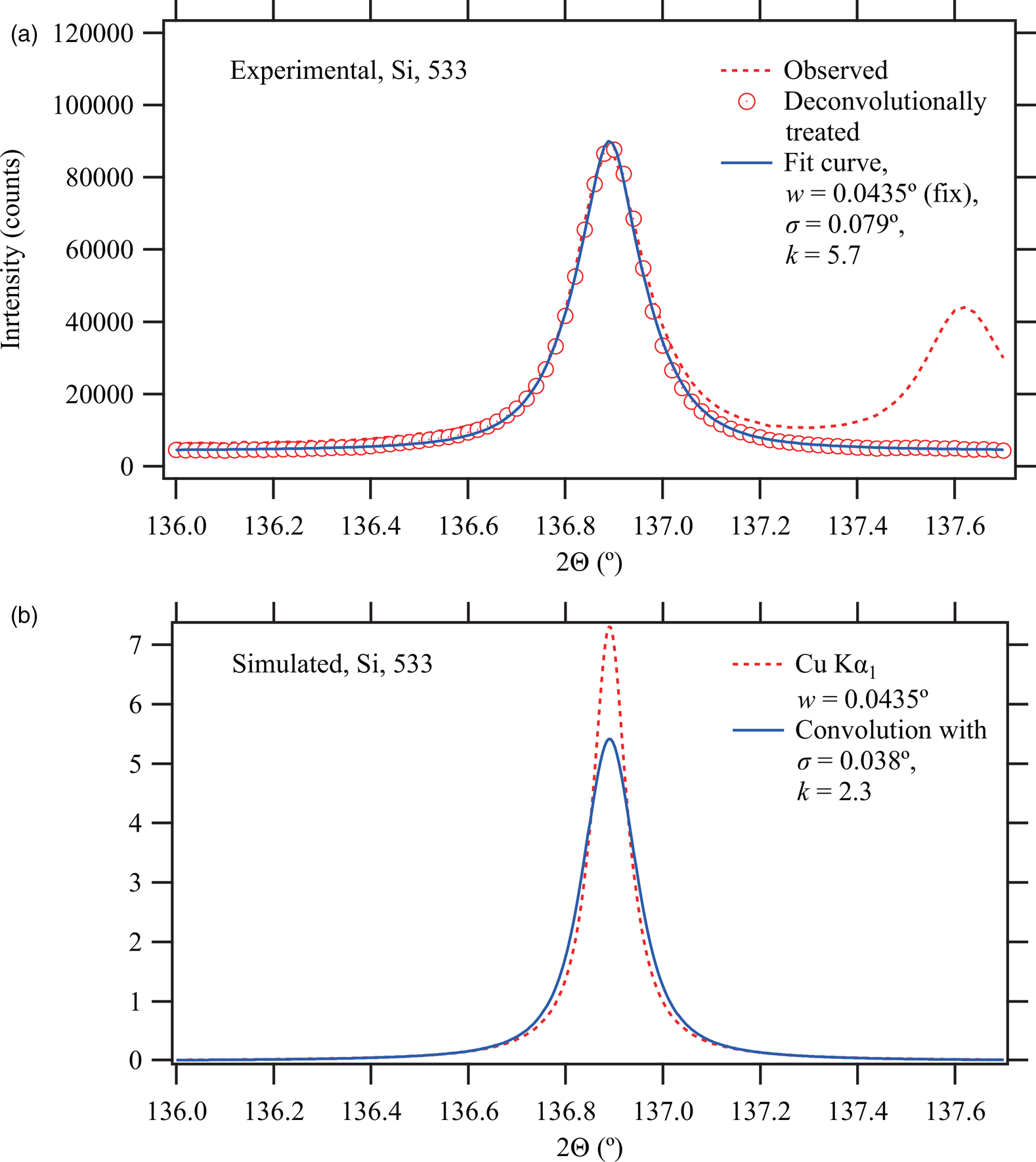
Figure 9. Comparison of experimental and simulated data for Si 533 reflection.
Single-peak curve-fitting analysis is applied to the deconvolutionally treated data with the profile model as the convolution of the Lorentzian and the symmetric function. The constant background, integrated intensity, peak location, standard deviation, and kurtosis are treated as variable parameters. The Lorentzian HWHM is treated as a fixed parameter on the analysis. The weighted nonlinear least-squares method based on the Levenberg–Marquardt algorithm (e.g., Press et al., Reference Press, Teukolsky, Vetterling and Flannery2007) is used for optimization, where it is assumed that the statistical errors in the intensities are equivalent to the square roots of the intensities. The fit curves are shown in Figures 7(a), 8(a), and 9(a). The optimized values of the varied parameters are listed in Table V.
TABLE V. Optimized values of fitting parameters. Constant background, integrated intensity, peak location, standard deviation σ, and kurtosis k of the instrumental component for three diffraction peaks of Si, 111, 422, and 533.

The peak profile in the deconvolutionally treated observed data generally exhibits such shape with sharp central peak and long tails as characteristics of high kurtosis of a symmetric function. The profile cannot be reproduced by the Voigt, pseudo-Voigt, or Pearson VII function, while the convolution model of the Lorentzian profile and the symmetric function with variable standard deviation and kurtosis certainly fits to the symmetrized observed peak profile.
It should also be noted that the apparent peak position of Si 422 peak is shifted by ![]() $0.02^\circ$ to higher angle side by the deconvolutional treatment, as can be seen in Figure 8(a). It is reasonably assigned to the correction of average sample-transparency peak shift estimated at
$0.02^\circ$ to higher angle side by the deconvolutional treatment, as can be seen in Figure 8(a). It is reasonably assigned to the correction of average sample-transparency peak shift estimated at ![]() ${-}0.021^\circ$ for the penetration depth of μ −1 = 0.137 mm of the Si powder specimen (Ida, Reference Ida2020b).
${-}0.021^\circ$ for the penetration depth of μ −1 = 0.137 mm of the Si powder specimen (Ida, Reference Ida2020b).
C. Discussions
Broader appearance of the deconvolutionally treated profile than the profile expected from geometrical parameters of the instrument, as commonly seen in Figures 7–9, suggests that some origins of instrumental broadening are missing, or any of the effects of assumed instrumental broadening are underestimated.
The assumptions about the spectroscopic profile of the source X-ray are most unlikely to be the dominant origins of the difference, because most of them are based on the results of reliable spectroscopic studies on characteristic X-rays (Deutsch et al., Reference Deutsch, Förster, Hölzer, Härtwig, Hämäläinen, Kao, Huotari and Diamant2004), even though the dependence of the observed difference in diffraction angles may appear similar to the spectroscopic broadening, proportional to tanΘ. It is suggested that the origin of the difference should be assigned to the assumptions about the instrument or the specimen.
If the underestimation about the axial-divergence effect should be dominant, the difference would appear more significant at lower and higher angles, because the standard deviation of the axial-divergence broadening should be proportional to ![]() $( {{\tan }^2{\rm \Theta } + 6/17 + {\cot }^2{\rm \Theta }} ) ^{1/2}$ (Ida, Reference Ida2020b), but the observed difference does not show such tendency.
$( {{\tan }^2{\rm \Theta } + 6/17 + {\cot }^2{\rm \Theta }} ) ^{1/2}$ (Ida, Reference Ida2020b), but the observed difference does not show such tendency.
The flat-specimen aberration has stronger effect at the lower angles, because the broadening should be proportional to ![]() $\cot {\rm \Theta }$ (Ida, Reference Ida2020b), but the results do not show larger difference at lower angles, either.
$\cot {\rm \Theta }$ (Ida, Reference Ida2020b), but the results do not show larger difference at lower angles, either.
The effect of sample transparency should have the standard deviation proportional to sin 2Θ, and should become maximum at ![]() $2{\rm \Theta } = 90^\circ$, but the observed difference appears a little more pronounced for the peak located at higher angles. On the other hand, it is also suggested that the difference should be assigned to the underestimation of the effects of sample transparency, because the aberration caused by the sample transparency has the highest kurtosis of six among the components of the assumed instrumental aberrations (Ida, Reference Ida2020b), and the optimized values of kurtosis to fit the observed peak profile are certainly larger than the expected values for the peaks at higher angles.
$2{\rm \Theta } = 90^\circ$, but the observed difference appears a little more pronounced for the peak located at higher angles. On the other hand, it is also suggested that the difference should be assigned to the underestimation of the effects of sample transparency, because the aberration caused by the sample transparency has the highest kurtosis of six among the components of the assumed instrumental aberrations (Ida, Reference Ida2020b), and the optimized values of kurtosis to fit the observed peak profile are certainly larger than the expected values for the peaks at higher angles.
Since a parameter related to the sample-transparency effect, linear attenuation coefficient μ, or penetration depth μ −1 depends on the estimated bulk density of the powder specimen, experimental errors are likely to be introduced to the assumed value of μ −1. There are other suspicious factors related to the sample-transparency effects. The assumed geometric model appears too simplified, and the effects of surface roughness and inhomogeneity of powder packing should affect the shape of the aberration function, but they are neglected in the current model. The linear attenuation coefficient should depend on the photon energy of X-ray, but the dependence is also neglected. It is suggested that studies focusing on sample preparation should be required to clarify the issues about the broadening effects of sample transparency.
It is still possible that the series of symmetric functions proposed in this study is not suitable for modeling the instrumental broadening effects of a realistic measurement system, because the series is designed mainly for the convenience of computation with the currently available numerical system. However, high flexibility, convenience for computation, unambiguous definition, and logical consistency will help further improvements in accuracy and efficiency on computation, and the reliability of analysis about powder diffraction data.
IV. CONCLUSION
A continuous series of symmetric single-peak profile models, the shapes of which are uniquely determined by the values of standard deviation and kurtosis, has been constructed. The series is composed of the truncated Gaussian, sheared Gaussian, and symmetric Rosin-Rammler-type functions. The rectangular shape for the kurtosis of –1.2, Gaussian shape for the kurtosis of 0, and symmetric exponential shape for the kurtosis of 3 are all included in the series. The peak shape can continuously be changed on variation of the kurtosis, and infinitely large kurtosis can be reproduced.
A practical method to evaluate the convolution of the symmetric functions with the Lorentzian function is described. The Voigt profile can be treated as a special case of the system expanded by the convolution with the Lorentzian function. The convolution model can be used as a peak profile model function for curve-fitting analysis. The model has been applied to the analysis of symmetrized diffraction peak profile treated by a deconvolutional method.
It is suggested that the treatment about the effects of sample transparency should be focused on for the improvement of accuracy of analysis of powder X-ray diffraction data collected with a measurement system based on the Bragg-Brentano geometry.
SUPPLEMENTARY MATERIAL
The supplementary material for this article can be found at https://doi.org/10.1017/S0885715621000567. Python codes for tabulation of Tables I, II, and III are given as “table1.py”, “table2.py”, and “table3.py”, respectively. A Python code for demonstration, including the convolution with the Lorentzian function as a callable function, the shape of which is uniquely determined by the Lorentzian half width w, and the standard deviation σ and kurtosis k of the symmetric (symmetrized) instrumental function, is given as “demo.py”.

