Hostname: page-component-78c5997874-t5tsf Total loading time: 0 Render date: 2024-10-28T04:18:58.135Z Has data issue: false hasContentIssue false

Steady solutions of quasi-geostrophic flows in basins, gulfs and channels on a β-plane

Published online by Cambridge University Press:  10 October 2024

Jeasson F. Gonzalez*
Affiliation:
Secretaría de Educación del Distrito Capital, Bogotá 110931, Colombia
L. Zavala Sansón
Affiliation:
Departamento de Oceanografía Física, CICESE, Ensenada 22860, México
F. Graef
Affiliation:
Departamento de Oceanografía Física, CICESE, Ensenada 22860, México
*
Email address for correspondence: [email protected]

Abstract

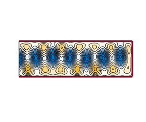
Nonlinear steady solutions of the barotropic quasi-geostrophic equation in basins, gulfs and channels on a $\beta$-plane are presented. The domains are rectangular with arbitrary aspect ratios. The two-dimensional solutions assume a linear relationship between the potential vorticity $q$ and the stream function $\psi$. The sign of the slope in the linear $q\unicode{x2013}\psi$ relationship defines two broad sets of solutions. For a positive slope, the solutions in a closed basin correspond to the inertial gyres derived by Fofonoff in 1954. The negative slope solutions consist of normal modes that can be resonant. For gulfs and channels, the conditions at the open boundaries are almost arbitrary flows entering or leaving the domain. Such conditions allow a great variety of solutions in the interior, characterised mainly by arrays of vortices with alternate signs. Several examples are presented and discussed.

Type
JFM Papers
Copyright
© The Author(s), 2024. Published by Cambridge University Press

1. Introduction

The governing equations of homogeneous and incompressible two-dimensional (2-D) flow in the limit of zero viscosity and no external forcing (Euler dynamics) admit steady, nonlinear solutions. From the vorticity equation, it is readily found that the nonlinear terms cancel out, implying a functional relationship between the vertical component of the vorticity and a suitably defined stream function (whose spatial derivatives provide the horizontal velocity components). This procedure has been known since the times of Stokes in 1842, and was successfully applied by Lamb and Chaplygin at the turn of the 20th century to derive nonlinear solutions of dipolar vortices in ideal 2-D flows (see a comprehensive discussion in Meleshko & van Heijst Reference Meleshko and van Heijst1994).

In the context of large-scale oceanographic flows, which present a predominantly 2-D behaviour due to the effects of the Earth's rotation, Fofonoff (Reference Fofonoff1954) applied the same procedure to study nonlinear solutions of steady inertial flows in a rectangular closed basin (with no forcing or dissipation). In the quasi-geostrophic $\beta$-plane approximation, the Fofonoff solutions consist of a linear relation between the potential vorticity $q$ and the stream function $\psi$, such that $q=\alpha ^2 \psi + \gamma$, where $\alpha ^2$ and $\gamma$ are free parameters. Here, $q=\omega + \beta y$, where $\omega$ is the relative vorticity, $\beta$ is the latitudinal gradient of the Coriolis parameter, and $y$ is the latitudinal coordinate (see e.g. Vallis Reference Vallis2017).

The so-called Fofonoff modes consist of closed circulations in a rectangular basin, whose characteristics are determined by constants $\alpha ^2$ and $\gamma$. The modes of oceanographic interest are characterised by a wide westward flow with a thin return current at either the northern or southern boundary (for the case of single gyres, see figure 1 in Fofonoff Reference Fofonoff1954), or at both boundaries (double gyre). Although the form of the Fofonoff solutions is highly idealised and is still far from representing actual oceanic flows, they became an important paradigm because they capture some essential features of basin-scale flows. For instance, inertial solutions illustrate the westward intensification of the circulation with no need to linearise the dynamical equation or use eddy viscosity terms, as in the wind-driven ocean in the Stommel model (Stommel Reference Stommel1948).

The Fofonoff solutions and, in general, nonlinear flows obeying a functional $q\unicode{x2013}\psi$ relationship are of interest for the following reasons.

  1. (i) Several studies based on more complex ocean dynamics have reported different flows’ tendencies to acquire characteristics similar to those of the Fofonoff modes. This behaviour is particularly remarkable in continuously forced turbulence (Griffa & Salmon Reference Griffa and Salmon1989; LaCasce Reference LaCasce2002; Zavala Sansón Reference Zavala Sansón2022) and problems with different viscous terms and boundary conditions (Cummins Reference Cummins1992; Wang & Vallis Reference Wang and Vallis1994).

  2. (ii) The linear $q\unicode{x2013}\psi$ relationship arises in different theoretical formulations, such as in the statistical mechanics theory for finite resolution models (e.g. spectrally truncated; see Salmon, Holloway & Hendershott Reference Salmon, Holloway and Hendershott1976). The $q\unicode{x2013}\psi$ linear correspondence is also found for decaying flow over random topography in quasi-geostrophic (Bretherton & Haidvogel Reference Bretherton and Haidvogel1976) and shallow-water (Merryfield, Cummins & Holloway Reference Merryfield, Cummins and Holloway2001; Zavala Sansón, González-Villanueva & Flores Reference Zavala Sansón, González-Villanueva and Flores2010) theories, as well as in the 2-D $\beta$-plane channel (Young Reference Young1987). Different vortex solutions based on equivalent linear relationships have been found through the years; for instance, the asymmetric Chaplygin dipole (Meleshko & van Heijst Reference Meleshko and van Heijst1994), the dipolar modon (Stern Reference Stern1975), and several analytical solutions of monopolar and dipolar vortices over mountains and valleys (Gonzalez & Zavala Sansón Reference Gonzalez and Zavala Sansón2021).

  3. (iii) Solutions with a linear $q\unicode{x2013}\psi$ relationship with opposite sign behave differently. In this case, there are normal mode solutions that can resonate, as discussed in the nonlinear stability analyses of Carnevale & Fredericksen (Reference Carnevale and Fredericksen1987) and in the shallow-water context with topography by LaCasce, Nøst & Isachsen (Reference LaCasce, Nøst and Isachsen2008).

  4. (iv) More general functional $q\unicode{x2013}\psi$ relationships have been studied in theoretical (Robert & Sommeria Reference Robert and Sommeria1991), numerical (Brands, Maassen & Clercx Reference Brands, Maassen and Clercx1999) and experimental (Trieling, van Heijst & Kizner Reference Trieling, van Heijst and Kizner2010) studies of 2-D turbulence and vortex dynamics.

This paper discusses new linear $q\unicode{x2013}\psi$ solutions for the quasi-geostrophic model on the $\beta$-plane for a homogeneous fluid on a flat bottom in three domains: a closed basin, an elongated gulf, and a channel. The gulf and the channel geometries allow very general inlet and outlet conditions. In addition, the solutions consider the linear $q\unicode{x2013}\psi$ relationship with positive and negative slopes. Thus a comprehensive family of analytical expressions is found.

Equilibrium states of oceanographic flows in different regions, domains and physical conditions have been studied in various works based on long-term observations or measurements. For instance, there is a semi-permanent anticyclonic vortex in the Lofoten Basin (Nordic Seas; Köhl Reference Köhl2007) and a cyclonic vortex at the Campeche Bay (Gulf of Mexico; Zavala Sansón, Sheinbaum & Pérez-Brunius Reference Zavala Sansón, Sheinbaum and Pérez-Brunius2018). Several gulfs and elongated bays in Earth's oceans exhibit a pattern of eddies along their axis, such as in the Aqaba Gulf (Berman, Paldor & Brenner Reference Berman, Paldor and Brenner2000), and the Bahia de Banderas canyon in the Mexican Pacific (Pantoja, Marinone & Filonov Reference Pantoja, Marinone and Filonov2017). In more significant scale gulfs, a train of eddies is commonly observed in the Red Sea (Zhan et al. Reference Zhan, Subramanian, Yao and Hoteit2014), the Gulf of Aden (Bower & Fratantoni Reference Bower and Fratantoni2002), and along the Gulf of California (Lavín et al. Reference Lavín, Castro, Beier and Godinez2013). Some ocean channels have a dipolar structure that transports mass along them, as reported by Wibowo et al. (Reference Wibowo, Tanjung, Rifardi, Mubarak, Yoswaty, Susanti, Muttaqin, Fajary and Anwika2022) for the Malacca Strait. The analytical solutions in this paper consist of an ample repertoire of different flow arrangements, some of which are of potential oceanographic interest because they resemble field observations.

The paper is structured as follows. In § 2, we present the steady and nonlinear quasi-geostrophic solutions based on a general $q\unicode{x2013}\psi$ linear relationship. The solutions for positive and negative slopes are shown. Section 3 evaluates and presents the two solutions for three flow domains: a closed basin, a gulf and a channel. Stability arguments for some solutions are presented. In § 4, we summarise and discuss the results.

2. Analytical solutions

We consider a homogeneous, incompressible and inviscid fluid described by the barotropic quasi-geostrophic model on the $\beta$-plane. Using a Cartesian coordinate system $(x,y)$ in which east and north coincide with the positive $x$ and $y$ directions, respectively, the dimensional quasi-geostrophic vorticity equation is

(2.1)\begin{equation} \frac{\partial}{\partial t} \nabla^2\psi + J(\psi,\nabla^2\psi+\beta y)=0, \end{equation}

where $\psi$ is the stream function, $J(a,b)\equiv \partial _xa\,\partial _yb -\partial _ya\,\partial _xb$ is the Jacobian operator, and $\nabla ^2 \equiv \partial _{xx} + \partial _{yy}$ is the Laplacian. The horizontal velocity components $(u,v)$ are defined as

(2.2a,b)\begin{equation} u={-}\partial_y \psi \quad \text{and} \quad v=\partial_x \psi, \end{equation}

so $\omega =\nabla ^2\psi$ is the vertical component of the relative vorticity. Recall that (2.1) represents the material conservation of potential vorticity, $q \equiv \nabla ^2 \psi + \beta y$.

The flow domain is a rectangle with meridional and zonal dimensions $L_y$ and $L_y/\epsilon$, respectively, with $\epsilon$ an arbitrary aspect ratio (figure 1). The domain is elongated zonally when $\epsilon <1$. A non-dimensional form of (2.1) is obtained using the scales

(2.3ad)\begin{equation} \psi=\hat{\psi}\psi_a,\quad y=L_yy_a,\quad x=\frac{L_y}{\epsilon}\,x_a,\quad t=\frac{L_y^2}{\epsilon\hat{\psi}}\,t_a, \end{equation}

where $\hat {\psi }$ is the stream function amplitude, and subscript $a$ denotes the non-dimensional variables. For steady flows, (2.1) without dimensions (and omitting subscript $a$ for notational convenience) is given by

(2.4)\begin{equation} J(\psi,\epsilon^2\,\partial_{xx}\psi + \partial_{yy}\psi + \hat{\beta}y) = 0. \end{equation}

We solve this nonlinear equation by assuming the linear $q\unicode{x2013}\psi$ relationship

(2.5)\begin{equation} q ={\pm}\alpha^2 \psi^\pm + \gamma, \end{equation}

where $\alpha$ and $\gamma$ are constants, and the sign before $\alpha ^2$ defines two types of solutions. Equation (2.5) implies that the stream function satisfies a non-homogeneous Helmholtz equation

(2.6) \begin{align} \epsilon^2\,\partial_{xx}\psi^{\pm} + \partial_{yy}\psi^{\pm} \mp \alpha^2 \psi^{\pm} ={-}\hat{\beta}y + \gamma, \end{align}

in which the inhomogeneity is provided by the $\beta$ effect and $\gamma$.

Figure 1. Rectangular zonal domain on a $\beta$-plane with aspect ratio $\epsilon$. The $x$ and $y$ directions are scaled with the meridional domain length $L_y$. The zonal walls are free-slip boundaries. The meridional walls can be closed or open.

We propose the separable solution

(2.7)\begin{equation} \psi^\pm(x,y) = F(x)\,G(y) + \eta(y), \end{equation}

yielding

(2.8)\begin{equation} \epsilon^2G\,\partial_{xx}F + F\,\partial_{yy}G \mp \alpha^2FG + \partial_{yy}\eta \mp \alpha^2\eta ={-}\hat{\beta}y + \gamma.\end{equation}

Equation (2.8) can be split into

(2.9)\begin{gather} \partial_{yy}\eta \mp \alpha^2\eta ={-}\hat{\beta}y + \gamma, \end{gather}
(2.10)\begin{gather}\epsilon^2G\,\partial_{xx}F + F\,\partial_{yy}G \mp \alpha^2FG = 0. \end{gather}

In the rest of this section, we present the solutions of (2.9) and (2.10), and then the stream functions $\psi ^{\pm }$ using (2.7). We will apply free-slip conditions at the zonal walls, i.e. at $y=0,1$. Afterwards, in § 3, we will show complete solutions for different conditions at the meridional boundaries $x=0,1$.

2.1. Solutions for $q=-\alpha ^2 \psi ^- + \gamma$

2.1.1. Solution for $\eta ^{-}(y)$

We require a free-slip condition at the zonal boundaries, implying a constant stream function there. Thus the complete problem for $\eta ^-(y)$ using (2.9) is

(2.11)\begin{equation} \partial_{yy}\eta^- + \alpha^2\eta^-{=} - \hat{\beta}y +\gamma,\quad \text{with}\ \eta^-(0)\equiv\eta_{S}, \eta^-(1)\equiv \eta_{N}. \end{equation}

Note that the solution admits different constant values at the southern and northern walls. Let $\eta ^-(y) = \eta ^-_h(y) + \eta ^-_p(y)$, where the homogeneous ($\eta ^-_h$) and particular ($\eta ^-_p$) solutions of (2.11) are

(2.12a,b)\begin{equation} \eta^-_h (y) = A_1\cos(\alpha y) + A_2\sin(\alpha y),\quad \eta^-_p (y) = (\gamma -\hat{\beta}y)/\alpha^2. \end{equation}

with $A_1$ and $A_2$ constants. To satisfy the boundary conditions, it is found that

(2.13a,b)\begin{equation} A_1 = \eta_S - \frac{\gamma}{\alpha^2}, \quad A_2 = \frac{\eta_N - (\eta_S -\gamma/\alpha^2)\cos(\alpha) -(\gamma - \hat{\beta})/ \alpha^2}{\sin(\alpha)}. \end{equation}

Therefore, the solution is

(2.14)\begin{align} & \eta^-(y;\alpha,\hat{\beta},\gamma,\eta_S,\eta_N) = \left(\eta_S - \frac{\gamma}{\alpha^2}\right)\cos(\alpha y) \end{align}
(2.15)\begin{align} &\quad +\frac{\eta_N - (\eta_S -\gamma/\alpha^2)\cos(\alpha) - (\gamma - \hat{\beta})/\alpha^2}{\sin(\alpha)}\sin(\alpha y)+(\gamma -\hat{\beta}y)/\alpha^2. \end{align}

2.1.2. Solution for $F^-(x)$ and $G^-(y)$

We can write (2.10) as

(2.16)\begin{equation} \frac{\partial_{yy}G^-}{G^-}={-}\left(\epsilon^2\,\frac{\partial_{xx}F^-}{F^-} + \alpha^2\right)=k,\end{equation}

with $k$ a constant. This gives the following equations for $G^-(y)$ and $F^-(x)$:

(2.17)\begin{gather} \partial_{yy}G^- -kG^- = 0, \end{gather}
(2.18)\begin{gather}\epsilon^2\,\partial_{xx}F^- + (\alpha^2 + k)F^- = 0. \end{gather}

We choose $k=-p^2$ with $p \in \mathbb {R}$ to obtain the solution for $G^-$ that satisfies the meridional boundary conditions:

(2.19)\begin{equation} G^-(y) = b_1\sin(py)+b_2\cos(py), \end{equation}

where $b_{1}$ and $b_{2}$ are constants. The no-normal flow condition $v(x,0)=v(x,1)=0$, or equivalently $\partial _x F^- G^-=0$ at the zonal boundaries, implies that $G^-(0)=G^-(1)=0$, which leads to

(2.20)\begin{equation} b_2=0,\quad p\equiv p_n=n{\rm \pi}\ (\text{with}\ n\ \text{integer}),\quad b_1=1\ (\text{arbitrary}), \end{equation}

and then

(2.21)\begin{equation} G^-_n(y) = \sin(p_ny). \end{equation}

The equation for $F^-(x)$ has $n$ solutions:

(2.22)\begin{equation} F^-_n(x; \alpha, \epsilon)=c_{1n}\sin(\lambda^-_n x) + c_{2n}\cos(\lambda^-_n x), \end{equation}

where $c_{1n}$, $c_{2n}$ and $\lambda ^-_n$ are complex constants, with the latter given by

(2.23)\begin{equation} \lambda^-_n=\left(\frac{\alpha^2-p_n^2}{\epsilon^2}\right)^{1/2}\in \mathbb{C}. \end{equation}

2.1.3. $\psi ^-$ solutions

Equation (2.10) has linearly independent solutions $F^-_nG^-_n$ for each mode $n$. Hence the more general solution is the sum $\sum _n^{\infty } F^-_nG^-_n$. Using (2.14), (2.21) and (2.22) in (2.7), we get the desired solution:

(2.24)\begin{align} \psi^- (x,y) &= \sum_{n=1}^{\infty} F^-_n(x) \sin(p_n y) + \eta^-(y) \nonumber\\ &= \sum_{n=1}^{\infty} [c_{1n}\sin(\lambda^-_n x) + c_{2n}\cos(\lambda^-_n x)] \sin(p_ny) + \left(\eta_S - \frac{\gamma}{\alpha^2}\right)\cos(\alpha y) \nonumber\\ &\quad +\frac{\eta_N - (\eta_S -\gamma/\alpha^2)\cos(\alpha) -(\gamma - \hat{\beta})/\alpha^2}{\sin(\alpha)} \sin(\alpha y) +(\gamma -\hat{\beta}y)/\alpha^2. \end{align}

2.2. Solutions for $q=\alpha ^2 \psi ^+ + \gamma$

Now we present the solutions of (2.9) and (2.10) using the positive sign to obtain $\psi ^+$. Given the similarity with the preceding subsection, some details will be omitted.

2.2.1. Solution for $\eta ^+(y)$

The problem for $\eta ^+(y)$ in (2.9) satisfying free-slip conditions at $y=0,1$ is given by

(2.25)\begin{equation} \partial_{yy}\eta^+ - \alpha^2\eta^+ = - \hat{\beta}y +\gamma, \quad \text{with}\ \eta^+(0)=\eta_{S}, \eta^+(1)=\eta_{N}. \end{equation}

The homogeneous ($\eta ^+_h$) and particular ($\eta ^+_p$) solutions of (2.25) are

(2.26a,b)\begin{equation} \eta^+_h (y) = A_1\cosh(\alpha y) + A_2\sinh(\alpha y),\quad \eta^+_p (y) ={-}(\gamma -\hat{\beta}y)/\alpha^2, \end{equation}

where constants $A_1$ and $A_2$ are obtained as in (2.12a,b). Thus the general solution satisfying the boundary conditions is

(2.27)\begin{align} & \eta^+(y;\alpha, \hat{\beta},\gamma,\eta_S,\eta_N) = \left(\eta_S + \frac{\gamma}{\alpha^2}\right)\cosh(\alpha y) \end{align}
(2.28)\begin{align} &\quad +\frac{\eta_N - (\eta_S +\gamma/\alpha^2)\cosh(\alpha) + (\gamma - \hat{\beta})/\alpha^2}{\sinh(\alpha)}\sinh(\alpha y) -(\gamma -\hat{\beta}y)/\alpha^2. \end{align}

2.2.2. Solution for $F^+(x)$ and $G^+(y)$

Equation (2.10) yields

(2.29)\begin{equation} \frac{\partial_{yy}G^+}{G^+}={-}\epsilon^2\,\frac{\partial_{xx}F^+}{F^+} + \alpha^2=k. \end{equation}

Separating the equation for $G^+(y)$ and choosing $k=-p^2$ yields the solution

(2.30)\begin{equation} G^+_n(y) = \sin(p_ny), \end{equation}

with $p_n=n{\rm \pi}$ again; from (2.21), note that $G^+_n(y)=G^-_n(y)$. The equation for $F^+(x)$ has solutions of the form

(2.31)\begin{equation} F^+_n(x; \alpha, \epsilon)=c_{1n}\sinh(\lambda^+_n x) + c_{2n}\cosh(\lambda^+_n x),\end{equation}

with the real constants

(2.32)\begin{equation} \lambda^+_n=\left(\frac{\alpha^2+p_n^2}{\epsilon^2}\right)^{1/2}\in \mathbb{R}. \end{equation}

2.2.3. $\psi ^+$ solutions

Finally, the stream function solution of (2.6) is given by

(2.33)\begin{align} & \psi^+ (x,y)= \sum_{n=1}^{\infty} F^+_n(x) \sin(p_n y) + \eta^+(y) \nonumber\\ &\quad =\sum_{n=1}^{\infty} [c_{1n}\sinh(\lambda^+_n x) + c_{2n}\cosh(\lambda^+_n x)]\sin(p_ny) + \left(\eta_S + \frac{\gamma}{\alpha^2}\right)\cosh(\alpha y) \nonumber\\ &\qquad +\frac{\eta_N - (\eta_S +\gamma/\alpha^2) \cosh(\alpha) +(\gamma - \hat{\beta})/\alpha^2}{\sinh(\alpha)}\sinh(\alpha y) -(\gamma -\hat{\beta}y)/\alpha^2. \end{align}

2.3. General properties

The steady solutions $\psi ^{\pm }$ given by (2.24) and (2.33) have the following properties.

  1. (i) The zonal mass flux depends only on the boundary conditions at the zonal walls, and is independent of the spatial coordinates:

    (2.34)\begin{equation} \int_0^1 u^{{\pm}}(x,y)\,{{\rm d}y}\equiv \int_0^1 \partial_y \psi^{{\pm}}(x,y)\,{{\rm d}y} = \eta_N - \eta_S. \end{equation}
    This result will be useful to prescribe open boundary conditions in gulfs and channels, as will be discussed in next section.
  2. (ii) The parameter $\gamma$ determines the meridional structure of the solutions $\psi ^{\pm }$, which is given by $\sin (n{\rm \pi} y)$ and functions $\eta ^{\pm }(y)$. In particular, when $\gamma =\hat {\beta }/2$ and considering $\eta _S=\eta _N=0$, the stream functions are antisymmetric with respect to $y=1/2$. This is verified by using $y^* = y-1/2$ (with $-1/2\le y^* \le 1/2$) and proving that

    (2.35)\begin{equation} \psi^{{\pm}}(x,y^*;\alpha,\epsilon,\hat{\beta},\gamma=\hat{\beta}/2) = \psi^{{\pm}}(x,-y^*;\alpha,\epsilon,\hat{\beta},\gamma=\hat{\beta}/2). \end{equation}
  3. (iii) To have a physical interpretation of $\alpha$, we assume that its dimensional value $\alpha _d$ (with units of 1/length) depends on the physical parameters involved in the problem: $\alpha _d = \alpha _d(\hat {\psi }, \beta, L_y)$. This implies that $\alpha _d = \sqrt {\beta L_y/\hat {\psi }}\equiv L_R^{-1}$, where $L_R$ is the Rhines scale (Rhines Reference Rhines1975). Thus

    (2.36)\begin{equation} \alpha = L_y\alpha_d =L_y/L_R.\end{equation}
    Henceforth, we consider solutions with $\alpha \geq 1$.

3. Solutions in basins, gulfs and channels

This section discusses the steady flow solutions $\psi ^{\pm }(x,y)$ (2.24) and (2.33) by prescribing suitable boundary conditions. These conditions can be free-slip walls or open boundaries.

3.1. Boundary conditions

Three domains are analysed: a closed basin, a gulf and an open channel (figure 2). For the three domains, the zonal walls ($y=0,1$) are free-slip, and the constant value of the stream function there is chosen to be zero:

(3.1a,b)\begin{equation} \psi^{{\pm}}(x,0) \equiv \eta_S = 0,\quad \psi^{{\pm}}(x,1) \equiv \eta_N = 0. \end{equation}

Recall, however, that the formulation allows $\eta _S,\eta _N \neq 0$.

Figure 2. Non-dimensional domains: (a) closed basin, (b) zonal gulf, (c) zonal channel.

The meridional conditions at $x=0,1$ are defined by prescribing a constant value of $\psi ^{\pm }$ at free-slip walls, or the meridional velocity $v=\partial _x\psi ^{\pm }$ for open boundaries. For the closed basin, the meridional boundaries are free-slip; the gulf has an open boundary at the west, and a closed one at the east; the channel has the western and eastern boundaries open. Thus the meridional conditions are as follows.

(3.2)\begin{gather} \mbox{Basins:}\quad \left\{\begin{gathered} \psi^{{\pm}}(0,y)=0, \\[3pt] \psi^{{\pm}}(1,y)=0. \end{gathered}\right. \end{gather}
(3.3)\begin{gather} \mbox{Gulfs:} \quad \left\{\begin{gathered} \partial_x\psi^{{\pm}}(0,y)= V_0\sin (s {\rm \pi}y), \\[3pt] \psi^{{\pm}}(1,y)= 0. \end{gathered}\right. \end{gather}
(3.4)\begin{gather} \mbox{Channels:} \quad \left\{\begin{gathered} \partial_x\psi^{{\pm}}(0,y)=V_W\sin (s_W {\rm \pi}y), \\[3pt] \partial_x\psi^{{\pm}}(1,y)=V_E\sin(s_E {\rm \pi}y). \end{gathered}\right. \end{gather}

The constants $V_0$, $V_W$ and $V_E$ for the gulf and the channel are arbitrary magnitudes of the meridional flow at the open boundaries, and parameters $s$, $s_W$ and $s_E$ are arbitrary natural numbers $1,2,3,\ldots.$ We specified the meridional velocity to ensure continuity of the stream function at the points $(0,0)$ and $(0,1)$. Specifying the zonal velocity could result in non-zero meridional velocity profiles at these points.

The meridional velocity component in the open boundaries must be zero at the intersections with the zonal walls because the normal flow is zero there. This feature is satisfied by the sinusoidal functions in (3.3) and (3.4), but any other continuous function with the same property is allowed. In addition, the property (2.34) guarantees that the net zonal flux is zero regardless of the form of the meridional component at the open boundaries. For instance, an arbitrary meridional velocity $v^+(0,y)$ at the western boundary will imply a zonal component $u^+(0,y)$ such that $\int _0^1 \partial _y \psi ^+(0,y) {{\rm d}y}=0$.

The $\psi ^{\pm }$ solutions (2.24) and (2.33) include infinite series, so the exact solutions correspond to $n \rightarrow \infty$. Thus the plots presented in subsequent subsections necessarily correspond to truncated solutions for a finite number of modes $N$. Hereafter, unless otherwise indicated, we assume $\hat {\beta }=100$, corresponding to $\beta \sim 2 \times 10^{-8}$ km$^{-1}$ s$^{-1}$, a length scale $L_y=1000$ km, and velocity $\hat {\psi }/L_y=0.2$ m s$^{-1}$. For these values, the Rhines scale is $L_R\sim 100$ km. We first present the $\psi ^+$ solutions to compare with the Fofonoff solutions. Afterwards, we examine the more complex structures obtained with $\psi ^-$.

3.2. $\psi ^+(x,y)$ solutions

3.2.1. Basins

From the $\psi ^+$ solution (2.33), the conditions (3.2) at the west and east boundaries are

(3.5)\begin{gather} \psi^+(0,y)=\sum_{n=1}^{\infty} c_{2n} \sin(p_ny) + \eta^+(y;\alpha,\hat{\beta},\gamma,0,0) = 0, \end{gather}
(3.6)\begin{gather}\psi^+(1,y)=\sum_{n=1}^{\infty} [c_{1n}\sinh(\lambda^+_n) + \cosh(\lambda^+_n)] \sin(p_ny) + \eta^+(y;\alpha,\hat{\beta},\gamma,0,0) = 0. \end{gather}

The values of $c_{1n}$ and $c_{2n}$ are determined by the method of Fourier coefficients, yielding

(3.7a,b)\begin{equation} c_{2n}=I^+(n),\quad c_{1n}\sinh(\lambda^+_n) + c_{2n}\cosh(\lambda^+_n) = I^+(n), \end{equation}

with the integral

(3.8)\begin{align} & I^+(n) ={-}2\int_0^1 \eta^+(y;\alpha,\hat{\beta},\gamma,0,0) \sin(p_n y)\,{{\rm d}y} \nonumber\\ &\quad = 2\int_0^1\left(-\frac{\gamma}{\alpha^2}\cosh(\alpha y) - \frac{-\gamma \cosh(\alpha y) + \gamma - \hat{\beta}}{\alpha^2\sinh(\alpha)}\sinh(\alpha y) - \frac{\hat{\beta}y - \gamma}{\alpha^2}\right)\sin(p_n y)\,{{\rm d}y} \nonumber\\[4pt] &\quad ={-}2\,\frac{\gamma}{\alpha^2}\left[\frac{\alpha \sinh(\alpha )\sin(n{\rm \pi}) -n{\rm \pi} \cosh(\alpha )\cos(n{\rm \pi} ) + n{\rm \pi}}{\alpha^2 + (n{\rm \pi})^2}\right] + \frac{2\gamma}{\alpha^2n{\rm \pi}}\,[1-\cos(n{\rm \pi})] \nonumber\\[4pt] &\qquad - 2\,\frac{\gamma -\gamma \cosh(\alpha ) - \hat{\beta}}{\alpha^2\sinh(\alpha)} \left[\frac{\alpha \cosh(\alpha)\sin(n{\rm \pi}) - n{\rm \pi} \sinh(\alpha)\cos(n{\rm \pi})}{\alpha^2 + (n{\rm \pi})^2}\right] \nonumber\\[4pt] &\qquad +\frac{2\hat{\beta}}{\alpha^2n{\rm \pi}}\cos(n{\rm \pi}). \end{align}

Hence solving the system (3.7a,b), the constants are

(3.9a,b)\begin{equation} c_{1n}=\frac{1-\cosh(\lambda^+_n)}{\sinh(\lambda^+_n)}\,I^+(n),\quad c_{2n}=I^+(n) . \end{equation}

Note that $I^+\rightarrow 0$ for $n \gg 1$, which implies $c_{1n},c_{2n}\rightarrow 0$, thus guaranteeing the absence of singular terms in the solution (2.33). In addition, $c_{1n}$ is always finite because of the limit $[1-\cosh (\lambda ^+_n)]/\sinh (\lambda ^+_n)\rightarrow 0$ for very small $\lambda _n^+$ values.

Consider first a square basin, $\epsilon =1$, which corresponds to the cases studied by Fofonoff (Reference Fofonoff1954). Figures 3(a,b) present the stream function and the velocity field for $\alpha = 10$ and two different $\gamma$ values. When $\gamma =0$, there is an intense anticyclonic cell next to the northern wall, as found by Fofonoff (see the lower panel of his figure 1, and also recall that Fofonoff showed an approximate boundary layer solution). For $\gamma =\hat {\beta }/2$, the solution corresponds to the well-known counter-rotating inertial gyres. Thus the Fofonoff structures are recovered satisfactorily with $N=10$ terms. Figures 3(c,d) show the stream function fields in a zonally elongated basin ($\epsilon <1$) for the same $\gamma$ values. The single anticyclonic gyre (figure 3c) and the double gyre (figure 3d) structure are found again but now stretched in the zonal direction. In this rectangular basin, the solutions converge with $N=55$ terms.

Figure 3. Stream function $\psi =\psi ^+(x,y)$ and velocity field in: (a,b) a square basin ($\epsilon =1$) with $\alpha =10$, $\gamma =0,\hat {\beta }/2$, $N=10$; and (c,d) an elongated domain ($\epsilon =0.25$) with $\alpha =1$, $\gamma =0,\hat {\beta }/2$, $N=55$.

The total kinetic energy and potential enstrophy are

(3.10)\begin{gather} \mathcal{E}(\alpha, \epsilon, \hat{\beta},\gamma) = \frac{1}{2}\int_{\mathcal{A}} |\nabla \psi^{{\pm}}|^2\,{\rm d}{\kern0.8pt}x\,{\rm d} y, \end{gather}
(3.11)\begin{gather}\mathcal{Z}(\alpha, \epsilon, \hat{\beta},\gamma) = \frac{1}{2}\int_{\mathcal{A}} (\nabla^2 \psi^{{\pm}}+\hat{\beta}y)^2 \,{\rm d}{\kern0.8pt}x\,{\rm d} y. \end{gather}

These global quantities as functions of $\alpha$ in the square basin are smooth, decaying functions, as seen in figure 4.

Figure 4. Kinetic energy (blue) and enstrophy (black) calculated with solutions $\psi ^+$ ($N=10$) as a function of $\alpha$ in a square basin, $\epsilon =1$: (a) $\gamma = 0$, (b) $\gamma =\hat {\beta }/2$. Both functionals are divided by $\hat {\beta }^2$ for visualisation purposes.

The curves reveal that the energy and enstrophy do not diverge for any $\alpha$ (we will see later that this is not the case for solutions $\psi ^-$). Similar energy and enstrophy curves are found in elongated domains (not shown).

3.2.2. Gulfs

For this domain, we consider an open boundary at the western side and a closed wall at the eastern side (figure 2b). Thus conditions (3.3) are

(3.12)\begin{gather} \partial_x\psi^+(0,y) = \sum_{n=1}^{\infty}c_{1n}\lambda^+_n\sin(p_n y) = V_0\sin(s{\rm \pi} y), \end{gather}
(3.13)\begin{gather}\psi^+(1,y) = \sum_{n=1}^{\infty}[c_{1n}\sinh(\lambda^+_n) + c_{2n}\cosh(\lambda^+_n)]\sin(p_n y) + \eta^+(y;\alpha,\hat{\beta},\gamma,0,0) = 0. \end{gather}

Using the Fourier method again, the solution of this system for $c_{1n}$ and $c_{2n}$ is

(3.14)\begin{gather} c_{1n} =\begin{cases} \displaystyle\frac{V_0}{{\rm \pi}\lambda_n^+}\left[\frac{\sin[(s - n){\rm \pi}]}{s-n} - \frac{\sin[(s + n){\rm \pi}]}{s+n} \right] & \text{if}\ s\neq n,\\ \displaystyle\frac{V_0}{\lambda_n^+} & \text{if}\ s = n, \end{cases}\end{gather}
(3.15)\begin{gather} c_{2n} =\begin{cases} \displaystyle\left(I^+(n) - \frac{V_0\sinh(\lambda^+_n)}{{\rm \pi}\lambda_n^+} \left[\frac{\sin[(s - n){\rm \pi}]}{s-n} - \frac{\sin[(s + n){\rm \pi}]}{s+n} \right]\right)/ \cosh(\lambda^+_n) & \text{if}\ s\neq n,\\ \displaystyle\left(I^+(n) - \dfrac{V_0\sinh(\lambda^+_n)}{\lambda_n^+}\right)/ \cosh(\lambda^+_n) & \text{if}\ s = n, \end{cases}\end{gather}

with $I^+(n)$ the integral (3.8).

Figure 5 presents the stream function and velocity fields in zonally elongated gulfs for four $\gamma$ values and using $V_0=0$. This condition corresponds to solutions where the total velocity at the entrance is purely zonal. In all cases, the flow remains zonal except near the eastern wall, where the fluid recirculates and turns westwards. The influence of $\gamma$ is, again, to generate a single anticyclonic cell ($\gamma =0$, figure 5a) or double gyres ($0<\gamma <\hat {\beta }$), as observed in the Fofonoff solutions.

Figure 5. Stream function $\psi = \psi ^+$ and velocity fields in an elongated gulf ($\epsilon =0.2$) with $\alpha =10$, for $\gamma$ values (a) $0$, (b) $\hat {\beta }/4$, (c) $\hat {\beta }/2$, and (d) $3\hat {\beta }/4$. The parameters at the western boundary are $V_0=0$ and $s=1$. The solutions are computed with $N=20$.

In figure 6, the velocity at the entrance is non-zonal, $V_0\neq 0$. In these cases, the non-parallel-flow condition at the gulf mouth affects only the meridional structure near the entrance, while the flow in the rest of the domain remains parallel until reaching the eastern wall. Again, these fields exhibit regions with closed circulations, resembling the Fofonoff flows according to the $\gamma$ value.

Figure 6. Same as figure 5 but for an elongated gulf ($\epsilon =0.5$) and a non-parallel-flow at the entrance, $V_0\neq 0$.

3.2.3. Channels

A channel, as illustrated in figure 2(c), is a domain with openings in both meridional boundaries. The meridional velocity components satisfy conditions (3.4):

(3.16)\begin{gather} \partial_x\psi^+(0,y) = \sum_{n=1}^{\infty}c_{1n}\lambda^+_n \sin(p_n y) = V_W\sin(s_W{\rm \pi} y), \end{gather}
(3.17)\begin{gather}\partial_x\psi^+(1,y) = \sum_{n=1}^{\infty} [c_{1n} \cosh(\lambda^+_n) + c_{2n} \sinh(\lambda^+_n)] \lambda^+_n \sin(p_n y) = V_E\sin(s_E{\rm \pi} y). \end{gather}

Following the procedures of the previous subsubsections, the coefficients $c_{1n}$ and $c_{2n}$ are

(3.18a,b) \begin{align} c_{1n} = \begin{cases} 0 & \text{if}\ s_W\neq n,\\ \dfrac{V_W}{\lambda_n^+} & \text{if}\ s_W = n, \end{cases}\quad c_{2n} =\begin{cases} -c_{1n}\cosh(\lambda_n^+)/\sinh(\lambda_n^+) & \text{if}\ s_E\neq n,\\ \left(\dfrac{V_E}{\lambda_n^+} -c_{1n}\cosh(\lambda_n^+)\right)/ \sinh(\lambda_n^+) & \text{if}\ s_E = n. \end{cases} \end{align}

In the case of purely parallel flow at the meridional boundaries, $V_W$ and $V_E$ are zero and the coefficients $c_{1n}$ and $c_{2n}$ become null. Then the $x$-dependent terms in the $\psi ^+$ solution (2.33) disappear too. Consequently, the stream function depends solely on the latitudinal coordinate as $\psi ^+(y)=\eta ^+(y;\alpha,\hat {\beta },\gamma,0,0)$. Thus

(3.19)\begin{equation} \psi^+(y) = \frac{\gamma}{\alpha^2}\cosh(\alpha y) + \frac{\gamma[1 - \cosh(\alpha)]-\hat{\beta}}{\alpha^2\sinh(\alpha)}\sinh(\alpha y) - \frac{\gamma-\hat{\beta}y}{\alpha^2}. \end{equation}

Figure 7 shows the zonal velocity profiles for different values of $\gamma$. The net zonal flow is zero, as anticipated from property (2.34). In particular, for $\gamma =0$, the flow near the northern boundary goes eastwards through a relatively thin region. Consequently, this boundary jet is compensated by westward motion at lower latitudes.

Figure 7. Zonal velocity profiles $u =u^+(y)=-\partial _y \psi ^+(y)$ calculated with (3.19) in a channel with parallel-flow conditions ($V_W = V_E = 0$) and different $\alpha$ values (coloured curves), for $\gamma$ values (a) $0$, (b) $\hat {\beta }/4$, (c) $\hat {\beta }/2$, and (d) $3\hat {\beta }/4$.

When the flow imposed at the meridional boundaries is not zonal ($V_W\neq 0$, $V_E\neq 0$), the $\psi ^+$ solutions exhibit a zonal structure. Figures 8(a,b) present two cases in an elongated domain where $V_W=V_E$ and $V_W=-V_E$, both with $s_W = s_E=1$. The resulting flows at the zonal boundaries enter and exit the channel, as shown in figures 8(c,d), which present the meridional profiles of the zonal velocity $u^+(y)$. In both examples, the flow is mostly zonal in the interior domain, except near the western and eastern ends, where the velocity acquires a meridional component to satisfy the boundary conditions (as found for the gulfs). Observe that the dominant part of the solution is a double gyre because $\gamma =\hat {\beta }/2$. Note also that the two cases exhibit different symmetries with respect to $x$ and $y$.

Figure 8. Stream function $\psi =\psi ^+$ and velocity fields in an elongated channel ($\epsilon =0.5$) with $\alpha =10$ and $\gamma =\hat {\beta }/2$ for boundary parameters $s_W=s_E=1$ and (a) $V_W=V_E=10$, (b) $V_W=-V_E=10$. (c,d) The zonal velocity profiles at $x=0$ and $x=2$. The solutions are obtained with $N=10$.

3.3. $\psi ^-(x,y)$ solutions

3.3.1. Basins

From the $\psi ^-$ solution (2.24), the conditions (3.2) at the meridional boundaries are

(3.20)\begin{gather} \psi^-(0,y)=\sum_{n=1}^{\infty} c_{2n} \sin(p_ny) + \eta^-(y;\alpha,\hat{\beta},\gamma,0,0) = 0, \end{gather}
(3.21)\begin{gather}\psi^-(1,y)=\sum_{n=1}^{\infty} [c_{1n}\sin(\lambda^-_n) + \cos(\lambda^-_n)] \sin(p_ny) + \eta^-(y;\alpha,\hat{\beta},\gamma,0,0) = 0, \end{gather}

where $\eta ^-(y)$ is given by (2.15). To determine the values of $c_{1n}$ and $c_{2n}$, we follow again the Fourier method used in § 3.2.1, which gives

(3.22a,b)\begin{equation} c_{1n} = \frac{1 - \cos(\lambda^-_n )}{\sin(\lambda^-_n )}\,I^-(n),\quad c_{2n} = I^-(n), \end{equation}

with the new integral

(3.23)\begin{align} I^-(n) &={-}2\int_0^1 \eta^-(y;\alpha,\hat{\beta},\gamma,0,0)\sin(p_n y)\,{{\rm d}y} \nonumber\\ &= 2\int_0^{1} \left(\frac{\gamma}{\alpha^2}\cos(\alpha y)- \frac{\gamma\cos(\alpha)-\gamma + \hat{\beta}}{\alpha^2 \sin(\alpha)}\sin(\alpha y)- \frac{\gamma -\hat{\beta}y}{\alpha^2}\right)\sin(p_ny) \,{{\rm d}y} \nonumber\\ &= \frac{\gamma}{\alpha^2}\left[\frac{\cos(\alpha-n{\rm \pi})}{\alpha-n{\rm \pi}} - \frac{\cos(\alpha+n{\rm \pi})}{\alpha+n{\rm \pi}} + \frac{1}{\alpha +n{\rm \pi}} - \frac{1}{\alpha - n{\rm \pi}}\right] - \frac{2\hat{\beta}}{\alpha^2n{\rm \pi}}\cos(n{\rm \pi}) \nonumber\\ &\quad -\frac{\gamma\cos(\alpha)-\gamma + \hat{\beta}}{\alpha^2\sin(\alpha)} \left[\frac{\sin(\alpha-n{\rm \pi})}{\alpha-n{\rm \pi}} - \frac{\sin(\alpha+n{\rm \pi})}{\alpha+n{\rm \pi}}\right] -\frac{2\gamma}{\alpha^2 n{\rm \pi}}\left[1-\cos(n{\rm \pi})\right]. \end{align}

If $\gamma =0$, then the coefficients $c_{1n}$ defined in (3.22a,b) are singular for $\lambda ^-_n = m{\rm \pi}$ with $m = 1, 3, 5, 7,\ldots$, and are zero when $m = 2,4,6,8,\ldots$, which is easily shown by L'Hopital's rule: $\lim _{\lambda ^-_n\rightarrow m{\rm \pi} }[1-\cos (\lambda ^-_n)]/\sin (\lambda ^-_n) = \lim _{\lambda ^-_n\rightarrow m{\rm \pi} } \sin (\lambda ^-_n)/\cos (\lambda ^-_n)$. Therefore, from the $\lambda ^-_n$ definition (2.23), the values of $\alpha$ where the singularities exist are

(3.24)\begin{equation} \alpha_{mn} = {\rm \pi}\sqrt{\epsilon^2 m^2 + n^2}. \end{equation}

To illustrate the singularities, figures 9(a,b) present the kinetic energy and potential enstrophy as functions of $\alpha$ for a square domain ($\epsilon =1$) and two characteristic values of $\gamma$. The curves demonstrate that the energy and enstrophy diverge when $\alpha =\alpha _{mn}$, so the corresponding solutions are forbidden. The plots also reveal that there are more singular values for $\gamma =0$ than for $\gamma =\hat {\beta }/2$ in the same $\alpha$ interval. Figures 9(c,d) present the energy and enstrophy curves but now as a function of the aspect ratio for zonally elongated domains, $0<\epsilon <1$, and fixed $\alpha$. The singularities $\epsilon _{mn}$ satisfy (3.24). The curves show that the density of singular values increases for more elongated domains, i.e. for $\epsilon \rightarrow 0$.

Figure 9. Kinetic energy (blue) and enstrophy (black) based on solutions $\psi ^-$ as functions of (a,b) $\alpha$ ($\epsilon =1$), and (c,d) $\epsilon$ ($\alpha =10$), for (a,c) $\gamma =0$, (b,d) $\gamma =\hat {\beta }/2$. The curves are obtained using $N=10$ terms. The dashed vertical lines indicate singularities.

The main consequence of having singularities is that the solutions corresponding to different $\alpha$ or $\epsilon$ intervals between singular values are steady flows of a specific class or characteristic structure, which is different from other classes. The large variety of admissible classes in solutions $\psi ^-$ is an essential difference compared to solutions $\psi ^+$.

To clarify the previous assertion, figure 10 presents the steady flow fields for different $\alpha$ values in a square basin ($\epsilon =1$) with $\gamma =0$. These plots correspond to minimum energy solutions in figure 9(a) and are representative of four different classes. Evidently, for larger $\alpha$, the flows have more and smaller vortical structures. A remarkable aspect is that there are no smooth transitions between the solutions of adjacent classes. For instance, all the solutions of the first class are characterised by a large anticyclonic cell (as in figure 10a), whilst the solutions of the second class are cyclonic vortices (as in figure 10b).

Figure 10. Stream function $\psi =\psi ^-(x,y)$ and velocity fields in a square basin ($\epsilon =1$) with $\gamma =0$, for (a$\alpha =1$, (b) $\alpha =6$, (c) $\alpha =12$, (d) $\alpha =18.7$. The solutions are truncated at $N=50$.

Figure 11 shows solutions in an elongated domain ($\epsilon = 0.4$) with different $\alpha$ and $\gamma$ values. It is observed again that bigger $\alpha$ implies more and smaller vortices, as can be seen by comparing figures 11(a,b) ($\alpha =10$) and figures 11(c,d) ($\alpha =20$). The effect of $\gamma$ has an influence on the north–south symmetry: the flow is asymmetrical for $\gamma =0$, and antisymmetrical with respect to $y=0.5$ for $\gamma =\hat {\beta }/2$ (as in the Fofonoff solutions).

Figure 11. Stream function $\psi =\psi ^-(x,y)$ and velocity fields in a rectangular basin ($\epsilon =0.4$) with: (a) $\alpha =10$, $\gamma =0$; (b) $\alpha =10$, $\gamma =\hat {\beta }/2$; (c) $\alpha =20$, $\gamma =0$; (d) $\alpha =20$, $\gamma =\hat {\beta }/2$. The solutions are truncated at $N=20$.

3.3.2. Gulfs

For this domain, the solutions (2.24) satisfy the meridional boundary conditions (3.3):

(3.25)\begin{gather} \partial_x\psi^-(0,y) = \sum_{n=1}^{\infty}c_{1n}\lambda^-_n \sin(p_n y) = V_0\sin(s{\rm \pi} y), \end{gather}
(3.26)\begin{gather}\psi^-(1,y) = \sum_{n=1}^{\infty}[c_{1n}\sin(\lambda^-_n) + c_{2n}\cos(\lambda^-_n)]\sin(p_n y) + \eta^-(y;\alpha,\hat{\beta},\gamma,0,0) = 0. \end{gather}

The coefficients are

(3.27) \begin{gather} c_{1n} =\begin{cases} \dfrac{V_0}{{\rm \pi}\lambda_n^-}\left[\dfrac{\sin[(s - n){\rm \pi}]}{s-n} - \dfrac{\sin[(s + n){\rm \pi}]}{s+n} \right] & \text{if}\ s\neq n,\\ \dfrac{V_0}{\lambda_n^-} & \text{if}\ s = n, \end{cases} \end{gather}
(3.28) \begin{gather} c_{2n} = \begin{cases} \left(I^-(n) - \dfrac{V_0\sin(\lambda^-_n)}{{\rm \pi}\lambda_n^-} \left[\dfrac{\sin[(s - n){\rm \pi}]}{s-n} - \dfrac{\sin[(s + n){\rm \pi}]}{s+n} \right]\right)/ \cos(\lambda^-_n) & \text{if}\ s\neq n,\\ \left(I^-(n) - \dfrac{V_0\sin(\lambda^-_n)}{\lambda_n^-}\right)/\cos(\lambda^-_n) & \text{if}\ s = n, \end{cases}\end{gather}

with $I^-(n)$ the integral (3.23). The coefficients $c_{2n}$ in (3.28) are singular when $\lambda ^-_n = (1/2 + m){\rm \pi}$ with $m = 0, 1, 2, 3,\ldots,$ i.e. for $\alpha$ satisfying

(3.29)\begin{equation} \alpha_{mn} = {\rm \pi}\sqrt{\epsilon^2 \left(\tfrac{1}{2} + m\right)^2 + n^2}. \end{equation}

Thus there are forbidden solutions in the gulf, as in the closed basin.

Figure 12 shows the stream function and velocity fields of steady flows in an elongated gulf ($\epsilon = 0.2$) for three $\alpha$ classes, and for each of them, four values of $\gamma$. To simplify, we examine cases with parallel flow at the western side, $V_0=0$. These choices illustrate the variety of different flow configurations. The plots reveal that a zonal sequence of vortices with alternating sign is a characteristic pattern of this domain (except for $\alpha =5$, $\gamma =\hat {\beta }/2$). As expected, the number of vortices increases with $\alpha$ for most of the $\gamma$ values. In each $\alpha$ class, the change of the flow pattern for different $\gamma$ is similar: the flow is almost unaltered from $\gamma =0$ to $\gamma =\hat {\beta }/4$, then becomes meridionally antisymmetric when $\gamma =\hat {\beta }/2$, and reverses for $\gamma =3\hat {\beta }/4$ (this sequence resembles what is observed in the Fofonoff solutions).

Figure 12. Stream function $\psi =\psi ^-(x,y)$ and velocity fields in a rectangular gulf ($\epsilon =0.2$) for different $\alpha$ and $\gamma$ values. In all cases, the meridional velocity amplitude at the western boundary is zero, $V_0=0$, so the entering flow is zonal. The solutions are obtained with $N=10$.

Figure 13 displays the zonal velocity profiles at the gulf entrance corresponding to the cases shown in figure 12. For $\alpha =5$, the fluid enters parallel to the zonal direction and exits through the central part for all the $\gamma$ values. In contrast, the zonal inflow and outflow for bigger $\alpha$ has a more irregular pattern and changes with $\gamma$.

Figure 13. Meridional profiles of the zonal velocity at the western entrance, $u =u^-(0,y)$, corresponding to the gulfs shown in figure 12.

3.3.3. Channels

This domain has meridional open boundaries. Conditions (3.4) are

(3.30)\begin{gather} \partial_x\psi^-(0,y) = \sum_{n=1}^{\infty}c_{1n}\lambda^-_n \sin(p_n y) = V_W\sin(s_W{\rm \pi} y), \end{gather}
(3.31)\begin{gather}\partial_x\psi^-(1,y) = \sum_{n=1}^{\infty} [c_{1n} \cos(\lambda^-_n) - c_{2n} \sin(\lambda^-_n)] \lambda^-_n \sin(p_n y) = V_E\sin(s_E{\rm \pi} y), \end{gather}

and solving the coefficients yields

(3.32)\begin{gather} c_{1n} =\begin{cases} \dfrac{V_W}{{\rm \pi}\lambda_n^-}\left[\dfrac{\sin[(s_W - n){\rm \pi}]}{s_W-n} - \dfrac{\sin[(s_W + n){\rm \pi}]}{s_W+n} \right] & \text{if}\ s\neq n,\\ \dfrac{V_W}{\lambda_n^-} & \text{if}\ s = n, \end{cases} \end{gather}
(3.33)\begin{gather} c_{2n} =\begin{cases} \dfrac{c_{1n}\cos(\lambda^-_n)-V_E\left[\dfrac{\sin[(s_E - n){\rm \pi}]}{s_E-n} - \dfrac{\sin[(s_E + n){\rm \pi}]}{s_E+n}\right]/{\rm \pi} \lambda^-_n}{\sin(\lambda^-_n)} & \text{if}\ s\neq n,\\ \dfrac{c_{1n}\cos(\lambda^-_n)-V_E/\lambda^-_n}{\sin(\lambda^-_n)} & \text{if}\ s = n. \end{cases} \end{gather}

As we found for the $\psi ^+$ solutions, the parallel-flow condition at both ends, $V_W=V_E=0$, implies that $c_{1n}=c_{2n}=0$ for all $n$, therefore the flow is purely zonal. The stream function is $\psi ^-=\eta ^-(y;\alpha,\hat {\beta },\gamma,0,0)$:

(3.34)\begin{equation} \psi^-(y) ={-} \frac{\gamma}{\alpha^2} \cos(\alpha y) - \frac{\gamma [1-\cos(\alpha)] - \hat{\beta}}{\alpha^2 \sin(\alpha)}\sin(\alpha y) + \frac{\gamma - \hat{\beta}y }{\alpha^2}. \end{equation}

Figure 14 shows the zonal velocity profiles calculated with (3.34) for several values of $\alpha$ and four values of $\gamma$. In all cases, the profiles represent eastward and westward zonal jets, and the number of jets increases with $\alpha$. This more complicated structure contrasts with the much smoother zonal jets found for solutions $\psi ^+$ in figure 7. A general feature of the $\psi ^-$ profiles is that the eastward jets are slightly more intense than their westward counterparts. Consequently, the eastward flows are narrower because the net zonal flux is zero, according to property (2.34).

Figure 14. Zonal velocity profiles $u =u^-(y)=-\partial _y \psi ^-(y)$ calculated with (3.34) in a channel with parallel-flow conditions ($V_W = V_E = 0$) and different $\alpha$ values (coloured curves), for $\gamma$ values (a) $0$, (b) $\hat {\beta }/4$, (c) $\hat {\beta }/2$, and (d) $3\hat {\beta }/4$.

To show solutions with non-parallel inflow/outlfow conditions, figures 15(a,b) present the steady flows for an elongated channel ($\epsilon = 0.5$), where $V_W, V_E\neq 0$, and $\alpha = 5$ and $10$, respectively. For these values, the flow structure remains similar for solutions with different values of $\gamma$, thus we show only examples with $\gamma =0$. For $\alpha =5$, the flow consists of a zonally elongated cell occupying mostly the southern part and two smaller cells at the north. For $\alpha = 10$, the structure is much more complex: there is a series of vortices with alternating sign along the channel, as we found in the basin and the gulf for higher $\alpha$ values.

Figure 15. Stream function $\psi =\psi ^-$ and velocity fields in an elongated gulf ($\epsilon =0.5$) with $\gamma =0$ and (a$\alpha =5$, (b) $\alpha =10$. The boundary parameters are $V_W = 10$, $s_W=1$ and $V_E = 20$, $s_E=3$. The solutions are truncated at $N=10$.

3.4. Stability arguments

In this section, we examine the stability of the solutions by considering the minimum enstrophy principle for quasi-geostrophic flows on a $\beta$-plane (Bretherton & Haidvogel Reference Bretherton and Haidvogel1976); for shallow-water flows, see Merryfield et al. (Reference Merryfield, Cummins and Holloway2001) and Zavala Sansón (Reference Zavala Sansón2010), and for vortical structures, see Leith (Reference Leith1984). The principle is based on the invariants of the vorticity equation (2.1): the global kinetic energy (3.10) and the generalised enstrophy integrals, the most important one being (3.11). The enstrophy cascades towards smaller scales, where viscous effects dissipate it. In contrast, energy cascades towards larger scales, and is virtually conserved. Thus the system tends towards a state of minimum enstrophy determined by the prescribed energy level. As mentioned by Young (Reference Young1987), this heuristic argument suggests that the configuration to which the flow evolves can be obtained by solving the variational principle of minimising the enstrophy subject to the given initial energy.

Following Young (Reference Young1987), we consider the enstrophy–energy curves $\mathcal {Z}$ versus $\mathcal {E}$ corresponding to the present solutions $\psi ^{\pm }$ for different $\alpha$ values (in our problem, $\alpha$ corresponds to the only Lagrange multiplier of the variational problem). Then we look for the minimum enstrophy solution for a given energy, which must be stable. Figures 16(a,b) show the energy–enstrophy relation for solutions $\psi ^-$ (solid curves for different $\alpha$ classes) and $\psi ^+$ (dashed curves) in the square basin ($\epsilon =1$) with $\gamma =0$ (figure 16a) and $\gamma =50$ (figure 16b). Consider first the case with $\gamma =0$ (figure 16a). There are three energy intervals where we find different minimum enstrophy solutions. Such solutions are $\psi ^+$ (dashed curve) for low energy values. In particular, the flow shown in figure 3(a) is stable. Note that the $\psi ^+$ branch merges with the first $\alpha$ class of the $\psi ^-$ solutions ($1<\alpha <4.4$). In the intermediate energy range, the minimum enstrophy solution corresponds to the $\psi ^-$ solutions of the third class $7<\alpha <9.9$ (figure 10a), and for even larger energies to the second class $4.4<\alpha <7$ (figure 10b). The $\psi ^-$ solutions in the other $\alpha$ classes are expected to be unstable. The energy–enstrophy curves for $\gamma =50$ and defined for different $\alpha$ classes (see figure 9) are presented in figure 16(b). Note that the flows shown in figures 3(b) and 10(c) are stable (minimum enstrophy for the corresponding energy), while that shown in figure 10(d) is unstable.

Figure 16. Enstrophy–energy curves for the solutions $\psi ^{\pm }$ in the square basin ($\epsilon =1$) with (a) $\gamma =0$ and (b) $\gamma =50$. Solid (dashed) curves represent $\psi ^-$ ($\psi ^+$) solutions. Colours distinguish the $\alpha$ classes of the $\psi ^-$ solutions found in figure 9. Labelled dots on the curves indicate some solutions presented in figures 3 and 10. Note that $\alpha ^-$ ($\alpha ^+$) represents the $\alpha$ value for solutions $\psi ^-$ ($\psi ^+$).

A similar analysis can be made for the solutions within the gulf with $\gamma =0$ and 50 (figures 17a,b). In these cases, we find again that the stable configurations for low energies correspond to $\psi ^+$ solutions. For larger energies, the minimum enstrophy solutions correspond to $\psi ^-$ for different $\alpha$ classes. Again, the labelled dots indicate whether the solutions presented in previous figures are stable or not. Interestingly, the $\psi ^+$ solutions in the elongated gulf shown in figures 5(a,c) are minimum enstrophy cases, as well as the $\psi ^-$ solutions presented in figures 12(a,c,g).

Figure 17. Same as figure 16, but now for a gulf with aspect ratio $\epsilon =0.2$. Labelled dots on the curves indicate some solutions presented in figures 5 and 12.

4. Discussion and conclusions

We derived nonlinear, stationary solutions of inviscid, quasi-geostrophic flows in different domains on a $\beta$-plane. The rectangular domains were a closed basin, a gulf, and a channel with arbitrary aspect ratio $\epsilon$. The solutions assume a linear relationship between the potential vorticity and the stream function, $q=\pm \alpha ^2 \psi ^{\pm } + \gamma$, so there are two broad sets of solutions: for $+\alpha ^2$, the $\psi ^+$ solution is (2.33), and for $-\alpha ^2$, the $\psi ^-$ function is (2.24). The $\psi ^+$ solutions in a closed basin correspond to the classical inertial gyres in a closed basin derived by Fofonoff (Reference Fofonoff1954). The $\psi ^-$ solutions in a closed domain consist of normal modes that can be resonant for specific discrete values of $\alpha$ (Carnevale & Fredericksen Reference Carnevale and Fredericksen1987; LaCasce et al. Reference LaCasce, Nøst and Isachsen2008). The parameter $\gamma$ modifies and shifts the resulting flow patterns in the meridional direction. The aspect ratio also strongly affects the elongation of the vortical structures.

One of the main features of the present solutions is that they admit a wide range of inward and outward flow conditions at the open boundaries of gulfs and channels. This characteristic is achieved by prescribing sinusoidal functions for the meridional velocity as boundary conditions in gulfs (3.3) and channels (3.4). The sine functions imply that the meridional velocity becomes null at the zonal walls, and the zonal transport is zero (otherwise, there would be non-zero divergence in the interior domain). A significant advantage of using these conditions is allowing multiple entries/exits to/from the domain. Also, they permit non-zonal flows at a given boundary.

The solutions consist of infinite sums. Therefore, the examples presented in the paper correspond to truncated solutions with $N$ terms. The convergence of the solutions depends on the choice of $N$. Some flows rapidly converge for $N=5$ or $10$ terms, while others require more than 50 terms. Not using sufficient terms might generate wrong values at the open boundaries.

The $\psi ^+$ solutions in the three domains present a gradual modification when changing $\alpha$. In these cases, the energy and potential enstrophy are smooth functions of $\alpha$. For this reason, the solutions are probably linearly or formally stable. In contrast, the $\psi ^-$ functions exhibit resonances for certain $\alpha$ values, at which the energy and potential enstrophy blow up. The flow patterns change abruptly for different $\alpha$ intervals delimited by the resonant values. Thus the $\psi ^-$ solutions are potentially unstable (Carnevale & Fredericksen Reference Carnevale and Fredericksen1987; LaCasce et al. Reference LaCasce, Nøst and Isachsen2008). However, a more detailed analysis in § 3.4 has shown that for specific prescribed energy values, there are minimum enstrophy solutions that are stable (Young Reference Young1987). Consequently, these states are plausible configurations in the oceanographic context. Hence we emphasise that the $\psi ^-$ solutions are as relevant and complementary as $\psi ^+$. An important case to mention is the pattern of alternating vortices along an elongated gulf, as shown in figure 12(a). Similar arrays have been observed in the ocean (see § 1), laboratory experiments (van Heijst, Davies & Davis Reference van Heijst, Davies and Davis1990; Maassen, Clercx & van Heijst Reference Maassen, Clercx and van Heijst2003) and numerical simulations of decaying flows (Zavala Sansón Reference Zavala Sansón2003) and forced 2-D flows (González Vera & Zavala Sansón Reference González Vera and Zavala Sansón2015). Another stable arrangement consisting of nearly symmetrical dipoles along the gulf is shown in figure 12(g).

Considering the vast amount of possible solutions, the minimum enstrophy analysis is limited to discussing only some particular cases. Nevertheless, the results are sufficient to show that several solutions are stable, especially those in elongated domains. Another point to take into account is that Young (Reference Young1987) studied a periodic $\beta$-plane channel and also considered the invariant zonal momentum to examine the enstrophy–energy curves for symmetric and non-symmetric solutions (wave solutions with zonal dependence). Future work might be devoted to performing a detailed analysis of the differences with the present results (with more general boundary conditions).

The present quasi-geostrophic solutions in flow domains with a zonal orientation have revealed various interesting patterns (arrays of alternating vortices, structures with predominant zonal motions, and recirculations near open boundaries). However, the ocean circulation is bounded not by zonal domains but by complex and oblique geometries oriented in any direction. Indeed, we expect that a tilted orientation of the domains will introduce new effects. This research line is under investigation, and the results will be published elsewhere.

Funding

This research received no specific grant from any funding agency, commercial or not-for-profit sectors.

Declaration of interests

The authors report no conflict of interest.

References

Berman, T., Paldor, N. & Brenner, S. 2000 Simulation of wind-driven circulation in the Gulf of Elat (Aqaba). J. Mar. Sys. 26, 349365.CrossRefGoogle Scholar
Bower, A.S. & Fratantoni, D.M. 2002 Gulf of Aden eddies and their impact on Red Sea water. Geophys. Res. Let. 29 (21), 14.CrossRefGoogle Scholar
Brands, H., Maassen, S.R. & Clercx, H.J.H. 1999 Statistical-mechanical predictions and Navier–Stokes dynamics of two-dimensional flows on a bounded domain. Phys. Rev. E 60 (3), 28642874.CrossRefGoogle Scholar
Bretherton, F.B. & Haidvogel, D. 1976 Two-dimensional turbulence over topography. J. Fluid Mech. 78, 129154.CrossRefGoogle Scholar
Carnevale, G.F. & Fredericksen, J.D. 1987 Nonlinear stability and statistical mechanics of flow over topography. J. Fluid Mech. 175, 157181.CrossRefGoogle Scholar
Cummins, P.F. 1992 Inertial gyres in decaying and forced geostrophic turbulence. J. Mar. Res. 50 (4), 545566.CrossRefGoogle Scholar
Fofonoff, N.P. 1954 Steady flow in a frictionless homogeneous ocean. J. Mar. Res. 13 (3), 254262.Google Scholar
Gonzalez, J.F. & Zavala Sansón, L. 2021 Quasi-geostrophic vortex solutions over isolated topography. J. Fluid Mech. 915, A64.CrossRefGoogle Scholar
González Vera, A.S. & Zavala Sansón, L. 2015 The evolution of a continuously forced shear flow in a closed rectangular domain. Phys. Fluids 27 (3), 034106.CrossRefGoogle Scholar
Griffa, A.C. & Salmon, R. 1989 Wind-driven ocean circulation and equilibrium statistical mechanics J. Mar. Res. 47 (3), 457492.CrossRefGoogle Scholar
van Heijst, G.J.F., Davies, P.A. & Davis, R.G. 1990 Spin-up in a rectangular container. Phys. Fluids A 2 (2), 150159.CrossRefGoogle Scholar
Köhl, A. 2007 Generation and stability of a quasi-permanent vortex in the Lofoten Basin. J. Phys. Oceanogr. 37 (11), 26372651.CrossRefGoogle Scholar
LaCasce, J.H. 2002 On turbulence and normal modes in a basin. J. Mar. Res. 60, 431460.CrossRefGoogle Scholar
LaCasce, J.H., Nøst, O.A. & Isachsen, P.E. 2008 Asymmetry of free circulations in closed ocean gyres. J. Phys. Oceanogr. 38 (2), 517526.CrossRefGoogle Scholar
Lavín, M.F., Castro, R., Beier, E. & Godinez, V.M. 2013 Mesoscale eddies in the southern Gulf of California during summer: characteristics and interaction with the wind stress. J. Geophys. Res. 118, 13671381.CrossRefGoogle Scholar
Leith, C.E. 1984 Minimum enstrophy vortices. Phys. Fluids 27 (6), 13881395.CrossRefGoogle Scholar
Maassen, S.R., Clercx, H.J.H. & van Heijst, G.J.F. 2003 Self-organization of decaying quasi-two-dimensional turbulence in stratified fluid in rectangular containers. J. Fluid Mech. 495, 1933.CrossRefGoogle Scholar
Meleshko, V.V. & van Heijst, G.J.F. 1994 On Chaplygin's investigations of two-dimensional vortex structures in an inviscid fluid. J. Fluid Mech. 272, 157182.CrossRefGoogle Scholar
Merryfield, W.J., Cummins, P.F. & Holloway, G. 2001 Equilibrium statistical mechanics of barotropic flow over finite topography. J. Phys. Oceanogr. 31 (7), 18801890.10.1175/1520-0485(2001)031<1880:ESMOBF>2.0.CO;22.0.CO;2>CrossRefGoogle Scholar
Pantoja, D.A., Marinone, S.G. & Filonov, A. 2017 Modeling the effect of a submarine canyon on eddy generation in Banderas Bay, Mexico. J. Coast. Res. 33 (3), 564572.CrossRefGoogle Scholar
Rhines, P.B. 1975 Waves and turbulence on $\beta$-plane. J. Fluid Mech. 69, 417443.CrossRefGoogle Scholar
Robert, R. & Sommeria, J. 1991 Statistical equilibrium states for two-dimensional flows. J. Fluid Mech. 229, 291310.CrossRefGoogle Scholar
Salmon, R., Holloway, G. & Hendershott, M.C. 1976 The equilibrium statistical mechanics of simple quasi-geostrophic models. J. Fluid Mech. 75 (4), 691703.CrossRefGoogle Scholar
Stern, M.E. 1975 Minimal properties of planetary eddies. J. Mar. Res. 33, 113.Google Scholar
Stommel, H. 1948 The westward intensification of wind-driven ocean currents. Trans. Am. Geophys. Union 29 (2), 202206.Google Scholar
Trieling, R.R., van Heijst, G.J.F. & Kizner, Z. 2010 Laboratory experiments on multipolar vortices in a rotating fluid. Phys. Fluids 22 (9), 094104.CrossRefGoogle Scholar
Vallis, G.K. 2017 Atmospheric and Oceanic Fluid Dynamics. Cambridge University Press.CrossRefGoogle Scholar
Wang, J. & Vallis, G.K. 1994 Emergence of Fofonoff states in inviscid and viscous ocean circulation models. J. Mar. Res. 52, 83127.CrossRefGoogle Scholar
Wibowo, M.A., Tanjung, A., Rifardi, Elizal, Mubarak, , Yoswaty, D., Susanti, R., Muttaqin, A.S., Fajary, F.R. & Anwika, Y.M. 2022 Understanding the mechanism of currents through the Malacca Strait study case 2020–2022: mean state, seasonal and monthly variation. IOP Conf. 1118, 012069.Google Scholar
Young, W.R. 1987 Selective decay of enstrophy and the excitation of barotropic waves in a channel. J. Atmos. Sci. 44 (19), 28042812.2.0.CO;2>CrossRefGoogle Scholar
Zavala Sansón, L. 2003 The two-dimensional character of spin-up in a rectangular container. Phys. Fluids 15 (6), 18111814.CrossRefGoogle Scholar
Zavala Sansón, L. 2010 Solutions of barotropic trapped waves around seamounts. J. Fluid Mech. 661, 3244.CrossRefGoogle Scholar
Zavala Sansón, L. 2022 Effects of mesoscale turbulence on the wind-driven circulation in a closed basin with topography. Geophys. Astrophys. Fluid Dyn. 116 (3), 159184.CrossRefGoogle Scholar
Zavala Sansón, L., González-Villanueva, A. & Flores, L.M. 2010 Evolution and decay of a rotating flow over random topography. J. Fluid Mech. 642, 159180.CrossRefGoogle Scholar
Zavala Sansón, L., Sheinbaum, J. & Pérez-Brunius, P. 2018 Single-particle statistics in the southern Gulf of Mexico. Geofís. Intl 57 (2), 139150.Google Scholar
Zhan, P., Subramanian, A.C., Yao, F. & Hoteit, I. 2014 Eddies in the Red Sea: a statistical and dynamical study. J. Geophys. Res. 119 (6), 39093925.CrossRefGoogle Scholar
Figure 0

Figure 1. Rectangular zonal domain on a $\beta$-plane with aspect ratio $\epsilon$. The $x$ and $y$ directions are scaled with the meridional domain length $L_y$. The zonal walls are free-slip boundaries. The meridional walls can be closed or open.

Figure 1

Figure 2. Non-dimensional domains: (a) closed basin, (b) zonal gulf, (c) zonal channel.

Figure 2

Figure 3. Stream function $\psi =\psi ^+(x,y)$ and velocity field in: (a,b) a square basin ($\epsilon =1$) with $\alpha =10$, $\gamma =0,\hat {\beta }/2$, $N=10$; and (c,d) an elongated domain ($\epsilon =0.25$) with $\alpha =1$, $\gamma =0,\hat {\beta }/2$, $N=55$.

Figure 3

Figure 4. Kinetic energy (blue) and enstrophy (black) calculated with solutions $\psi ^+$ ($N=10$) as a function of $\alpha$ in a square basin, $\epsilon =1$: (a) $\gamma = 0$, (b) $\gamma =\hat {\beta }/2$. Both functionals are divided by $\hat {\beta }^2$ for visualisation purposes.

Figure 4

Figure 5. Stream function $\psi = \psi ^+$ and velocity fields in an elongated gulf ($\epsilon =0.2$) with $\alpha =10$, for $\gamma$ values (a) $0$, (b) $\hat {\beta }/4$, (c) $\hat {\beta }/2$, and (d) $3\hat {\beta }/4$. The parameters at the western boundary are $V_0=0$ and $s=1$. The solutions are computed with $N=20$.

Figure 5

Figure 6. Same as figure 5 but for an elongated gulf ($\epsilon =0.5$) and a non-parallel-flow at the entrance, $V_0\neq 0$.

Figure 6

Figure 7. Zonal velocity profiles $u =u^+(y)=-\partial _y \psi ^+(y)$ calculated with (3.19) in a channel with parallel-flow conditions ($V_W = V_E = 0$) and different $\alpha$ values (coloured curves), for $\gamma$ values (a) $0$, (b) $\hat {\beta }/4$, (c) $\hat {\beta }/2$, and (d) $3\hat {\beta }/4$.

Figure 7

Figure 8. Stream function $\psi =\psi ^+$ and velocity fields in an elongated channel ($\epsilon =0.5$) with $\alpha =10$ and $\gamma =\hat {\beta }/2$ for boundary parameters $s_W=s_E=1$ and (a) $V_W=V_E=10$, (b) $V_W=-V_E=10$. (c,d) The zonal velocity profiles at $x=0$ and $x=2$. The solutions are obtained with $N=10$.

Figure 8

Figure 9. Kinetic energy (blue) and enstrophy (black) based on solutions $\psi ^-$ as functions of (a,b) $\alpha$ ($\epsilon =1$), and (c,d) $\epsilon$ ($\alpha =10$), for (a,c) $\gamma =0$, (b,d) $\gamma =\hat {\beta }/2$. The curves are obtained using $N=10$ terms. The dashed vertical lines indicate singularities.

Figure 9

Figure 10. Stream function $\psi =\psi ^-(x,y)$ and velocity fields in a square basin ($\epsilon =1$) with $\gamma =0$, for (a$\alpha =1$, (b) $\alpha =6$, (c) $\alpha =12$, (d) $\alpha =18.7$. The solutions are truncated at $N=50$.

Figure 10

Figure 11. Stream function $\psi =\psi ^-(x,y)$ and velocity fields in a rectangular basin ($\epsilon =0.4$) with: (a) $\alpha =10$, $\gamma =0$; (b) $\alpha =10$, $\gamma =\hat {\beta }/2$; (c) $\alpha =20$, $\gamma =0$; (d) $\alpha =20$, $\gamma =\hat {\beta }/2$. The solutions are truncated at $N=20$.

Figure 11

Figure 12. Stream function $\psi =\psi ^-(x,y)$ and velocity fields in a rectangular gulf ($\epsilon =0.2$) for different $\alpha$ and $\gamma$ values. In all cases, the meridional velocity amplitude at the western boundary is zero, $V_0=0$, so the entering flow is zonal. The solutions are obtained with $N=10$.

Figure 12

Figure 13. Meridional profiles of the zonal velocity at the western entrance, $u =u^-(0,y)$, corresponding to the gulfs shown in figure 12.

Figure 13

Figure 14. Zonal velocity profiles $u =u^-(y)=-\partial _y \psi ^-(y)$ calculated with (3.34) in a channel with parallel-flow conditions ($V_W = V_E = 0$) and different $\alpha$ values (coloured curves), for $\gamma$ values (a) $0$, (b) $\hat {\beta }/4$, (c) $\hat {\beta }/2$, and (d) $3\hat {\beta }/4$.

Figure 14

Figure 15. Stream function $\psi =\psi ^-$ and velocity fields in an elongated gulf ($\epsilon =0.5$) with $\gamma =0$ and (a$\alpha =5$, (b) $\alpha =10$. The boundary parameters are $V_W = 10$, $s_W=1$ and $V_E = 20$, $s_E=3$. The solutions are truncated at $N=10$.

Figure 15

Figure 16. Enstrophy–energy curves for the solutions $\psi ^{\pm }$ in the square basin ($\epsilon =1$) with (a) $\gamma =0$ and (b) $\gamma =50$. Solid (dashed) curves represent $\psi ^-$ ($\psi ^+$) solutions. Colours distinguish the $\alpha$ classes of the $\psi ^-$ solutions found in figure 9. Labelled dots on the curves indicate some solutions presented in figures 3 and 10. Note that $\alpha ^-$ ($\alpha ^+$) represents the $\alpha$ value for solutions $\psi ^-$ ($\psi ^+$).

Figure 16

Figure 17. Same as figure 16, but now for a gulf with aspect ratio $\epsilon =0.2$. Labelled dots on the curves indicate some solutions presented in figures 5 and 12.