Hostname: page-component-78c5997874-4rdpn Total loading time: 0 Render date: 2024-11-17T16:15:58.986Z Has data issue: false hasContentIssue false

Experimental measurement of spatio-temporally resolved energy dissipation rate in turbulent Rayleigh–Bénard convection

Published online by Cambridge University Press:  27 March 2024

Fang Xu
Affiliation:
Centre for Complex Flows and Soft Matter Research, Southern University of Science and Technology, Shenzhen 518055, PR China Department of Mechanics and Aerospace Engineering, Southern University of Science and Technology, Shenzhen 518055, PR China
Lu Zhang
Affiliation:
Centre for Complex Flows and Soft Matter Research, Southern University of Science and Technology, Shenzhen 518055, PR China Department of Mechanics and Aerospace Engineering, Southern University of Science and Technology, Shenzhen 518055, PR China
Ke-Qing Xia*
Affiliation:
Centre for Complex Flows and Soft Matter Research, Southern University of Science and Technology, Shenzhen 518055, PR China Department of Mechanics and Aerospace Engineering, Southern University of Science and Technology, Shenzhen 518055, PR China Department of Physics, Southern University of Science and Technology, Shenzhen 518055, PR China
*
Email address for correspondence: [email protected]

Abstract

We report a home-built velocity-gradient-tensor-resolved particle image velocimetry (VGTR-PIV) system which spatio-temporally resolves all components of the velocity gradient tensor. This technique is applied to the paradigmatic turbulent Rayleigh–Bénard convection system in a cylindrical cell at three representative positions, i.e. centre, side and bottom regions. The VGTR-PIV system allows us to directly measure, for the first time, the spatio-temporally resolved energy dissipation rate and enstrophy in turbulent thermal convection. In the experiment, the Rayleigh number $Ra$ varied in the range $2 \times 10^8 \leqslant Ra \leqslant 8 \times 10^9$ and the Prandtl number $Pr$ was fixed at $Pr = 4.34$. Compared with the fully resolved energy dissipation rate $\varepsilon$, the pseudo-dissipation provides the best estimate within $3\,\%$, the planar (two-dimensional) surrogate has a larger relative error and the one-dimensional surrogate leads to the largest error. The power-law scalings of the time-averaged energy dissipation rate with the Rayleigh number follow $\langle \varepsilon _c \rangle _t / (\nu ^3 H^{-4}) = 9.86 \times 10^{-6} Ra^{1.54 \pm 0.02}$, $\langle \varepsilon _s \rangle _t / (\nu ^3 H^{-4}) = 9.26 \times 10^{-3} Ra^{1.25 \pm 0.02}$ and $\langle \varepsilon _b \rangle _t / (\nu ^3 H^{-4}) = 2.70 \times 10^{-2} Ra^{1.23 \pm 0.02}$ in the centre, side and bottom regions, respectively where $\nu$ is dynamic viscosity and $H$ is cell height. These scaling relations, along with our earlier measured time-averaged energy dissipation rate at the bottom wall surface $\langle \varepsilon _w \rangle _t / (\nu ^3 H^{-4}) = 9.65 \times 10^{-2} Ra^{1.25 \pm 0.02}$ (J. Fluid Mech., vol. 947, 2022, A15), provide important constraints against which theoretical models may be tested. For the centre and side locations in the convection cell, the probability density functions (p.d.f.s) of the energy dissipation rate and enstrophy both follow a stretched exponential distribution. For the bottom region, the p.d.f.s of dissipation and enstrophy exhibit a stretched exponential distribution outside the viscous boundary layer and an exponential distribution inside the viscous boundary layer. It is also found that extreme events with high dissipation are the most intermittent in the side region, whereas the bottom region is less intermittent than the cell centre.

Type
JFM Papers
Copyright
© The Author(s), 2024. Published by Cambridge University Press

1. Introduction

Most flows occurring in nature and engineering applications are turbulent. In turbulent flows, the kinetic energy of a fluid is dissipated at the smallest scales owing to molecular viscosity. The energy dissipation rate, perhaps the most crucial quantity in the study of turbulence, characterises the transfer rate from kinetic energy to heat via molecular viscosity and is defined as

(1.1)\begin{align} \varepsilon = 2 \nu s_{ij} s_{ij}&= \nu \left[ \left(\frac{\partial u}{\partial y}\right)^2 + \left(\frac{\partial u}{\partial z}\right)^2 + \left(\frac{\partial v}{\partial x}\right)^2 + \left(\frac{\partial v}{\partial z}\right)^2 + \left(\frac{\partial w}{\partial x}\right)^2 + \left(\frac{\partial w}{\partial y}\right)^2 \right.\nonumber\\ &\quad + \left. 2 \left( \frac{\partial u}{\partial x}\right)^2 + 2 \left(\frac{\partial v}{\partial y}\right)^2 + 2 \left(\frac{\partial w}{\partial z}\right)^2 + 2 \frac{\partial u}{\partial y} \frac{\partial v}{\partial x} + 2 \frac{\partial u}{\partial z} \frac{\partial w}{\partial x} + 2 \frac{\partial v}{\partial z} \frac{\partial w}{\partial y} \right], \end{align}

where $\nu$ is the kinematic viscosity of the working fluid, $s_{ij} = (\partial u_i / \partial x_j + \partial u_j / \partial x_i) / 2$ is a component of the strain rate tensor $\boldsymbol {S}$, $u_i$ is the velocity component (i.e. u, v or w) and summation over repeated indices is implied. The energy dissipation rate has been widely studied in systems such as homogeneous and isotropic turbulence, Taylor–Couette flow, von Kármán swirling flow and turbulent boundary layers. The statistics of the energy dissipation rate are closely related to intermittency and energy cascades (Frisch Reference Frisch1995). The study of dissipation has promoted developments of many turbulence theories and models, such as the Richardson cascade model (Richardson Reference Richardson1922), Kolmogorov phenomenological theory (Kolmogorov Reference Kolmogorov1962) and turbulence modelling (Launder & Spalding Reference Launder and Spalding1974). Important as it is to access the instantaneous energy dissipation rate, all nine components of the velocity gradient tensor need to be resolved simultaneously, which is challenging experimentally. Thus, there is very limited work on measuring the energy dissipation rate without resorting to some assumptions (Wang et al. Reference Wang, Yang, Wu, Ma, Peng, Liu and Wang2021). In this paper, we present a measurement system which is able to spatio-temporally resolve the full velocity gradient tensor down to the Kolmogorov length and time scales while making long-term measurements at the same time. We demonstrate this technique using the system of turbulent thermal convection.

Turbulent thermal convection is ubiquitous in both natural phenomena and industrial applications. Rayleigh–Bénard convection (RBC), as a paradigmatic system for studying turbulent thermal convection, concerns a fluid layer between two horizontal plates which is heated from below and cooled from above. The RBC system has been studied extensively, focusing on both fundamentals and applications of turbulent flows (Ahlers, Grossmann & Lohse Reference Ahlers, Grossmann and Lohse2009; Lohse & Xia Reference Lohse and Xia2010; Chillà & Schumacher Reference Chillà and Schumacher2012; Xia Reference Xia2013; Xia et al. Reference Xia, Huang, Xie and Zhang2023a). Given the geometry of the convection cell, the control parameters of the RBC system are the Rayleigh number $Ra$ and the Prandtl number $Pr$

(1.2a,b)\begin{equation} Ra = \frac{\alpha_T g H^3 \Delta T} {\nu \kappa} ;\quad Pr = \frac{\nu} {\kappa}, \end{equation}

where $\alpha _T$ and $\kappa$ are the thermal expansion coefficient and the thermal diffusivity of the working fluid, $g$ is the gravitational acceleration, $H$ is the cell height and $\Delta T$ is the temperature difference across the fluid layer. As a closed system, there exists an exact balance between the volume-averaged energy dissipation rate and the global heat transport in RBC (Shraiman & Siggia Reference Shraiman and Siggia1990)

(1.3)\begin{equation} \langle \varepsilon \rangle_{V} = \frac{\nu^3}{H^4} (Nu - 1) \frac{Ra}{Pr^2}, \end{equation}

where the operator $\langle {\cdot } \rangle _{V}$ indicates volume averaging. This relation highlights the important role of energy dissipation rate in understanding and modelling the RBC system.

By assuming homogeneity and isotropy within the local measurement volume, Ni, Huang & Xia (Reference Ni, Huang and Xia2011) obtained the ensemble-averaged energy dissipation rate by conducting particle tracking velocimetry (PTV) measurements in the central region and found a power-law scaling $\langle \varepsilon \rangle _t \sim Ra^{1.55 \pm 0.02}$. They also observed a local balance between the energy dissipation rate and the convective heat flux in the centre. Subsequently, Li et al. (Reference Li, Huang, Ni and Xia2021) measured the ensemble-averaged energy dissipation rate in two $({\rm 50}\ {\rm mm})^3$ plume-abundant regions with their edges 15 mm away from the sidewall or the bottom plate and found a power-law scaling $\langle \varepsilon \rangle _t \sim Ra^{1.34 \pm 0.07}$ in both regions. Although direct numerical simulation is able to resolve the local energy dissipation rate, due to the limited computing resources, numerical simulations cannot provide long-term statistics, especially in the side or bottom regions where local homogeneity does not apply (Verzicco & Camussi Reference Verzicco and Camussi2003; Zhang, Zhou & Sun Reference Zhang, Zhou and Sun2017; Vishnu, De & Mishra Reference Vishnu, De and Mishra2022). To the best of our knowledge, no experimental work has been able to spatio-temporally resolve the energy dissipation rate in turbulent thermal convection. In the present work, we construct an advanced velocity-gradient-tensor-resolved particle image velocimetry (VGTR-PIV) system that has high spatial and temporal resolutions down to the Kolmogorov scales, is capable of long-term sampling and is versatile enough to be applied to different representative regions in the thermal convection system. The reported results regarding the energy dissipation rate in most of the previous numerical studies are based on volume averages, some over a significant portion and some over the whole volume, of the system. This makes it difficult to directly compare results from those numerical results with pointwise measurements. On the other hand, as a closed system, the scaling and probability density functions (p.d.f.s) of most physical quantities in turbulent RBC are position dependent. The strong position dependence makes volume averaging not very meaningful for many physical quantities and highlights the advantages of pointwise measurements.

The remainder of this paper is organised as follows. We present the experimental set-up, data acquisition and processing techniques for the spatio-temporally resolved energy dissipation rate measurement facility (VGTR-PIV system) in § 2. Our main results are presented in § 3, which is divided into four subsections. In § 3.1, we present results on the properties of velocity gradient tensor components. In § 3.2, we compare one-dimensional, two-dimensional and pseudo-surrogates of the energy dissipation rate. In § 3.3, we present and discuss the Rayleigh number dependence of the energy dissipation rate and the Reynolds number. In § 3.4, we analyse statistical properties of the energy dissipation rate and enstrophy. Finally, we summarise our findings and conclude in § 4.

2. The experimental set-up

Xu, Zhang & Xia (Reference Xu, Zhang and Xia2022) measured the full velocity profile at the intersection of two orthogonal vertical planes above the centre of the bottom plate. The energy dissipation rate at the centre of the bottom plate was obtained using the wall-shear stress vector. The present rig was built on that system with three orthogonal measurement planes using the same convection cell. For ease of reference, we provide more details of the convection cell. As shown in figure 1, it is a cylinder with its height and inner diameter both being 188 mm (unit aspect ratio). A water-filling square jacket is fitted around the Plexiglas sidewall to reduce image distortion. The bottom plate is made of a 30 mm thick copper disc with a black-nickel-plated surface. The top plate is made of a 5 mm thick sapphire disc to ensure both high thermal conductivity ($\lambda _f \approx 42\ {\rm W}\ ({\rm m}\ {\rm K})^{-1}$) and optical access from above. The temperature of the top plate is measured at the side of the sapphire disc by four evenly distributed thermistors. The bottom plate temperature is measured by four embedded thermistors. The thermistors (OMEGA 44031) used to measure the temperatures of the top and bottom plates have an accuracy of $0.01$ K and a response time of 1 s. We applied another type of thermistor (TE Connectivity NTC), which has a diameter of $0.2$ mm and a response time of 30 ms, to measure the bulk temperature. Over the sapphire plate, there is a cooling chamber for water circulation. Compared with the previous experimental set-up (Xu et al. Reference Xu, Zhang and Xia2022; Xia, Xu & Zhang Reference Xia, Xu and Zhang2023b), the current rig enables simultaneous optical measurements in three orthogonal planes, with sampling time smaller than the Kolmogorov time scale and spatial resolution smaller than the Kolmogorov length scale, making it possible to spatio-temporally resolve the velocity gradient tensor and the energy dissipation rate. The convection cell is insulated inside a thermostat to minimise heat exchange between the convection system and its surroundings, and the thermostat temperature is kept the same as the bulk temperature, i.e. $40\,^\circ {\rm C}$. The Cartesian coordinate system has its origin at the measurement position (centre, side or bottom), $x\unicode{x2013}y$ being the horizontal plane and $z$ axis pointing upward.

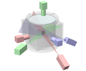
Figure 1. Sketch of the cylindrical convection cell, the VGTR-PIV system and the Cartesian coordinates. The enlarged drawing shows a sample of the highly fluctuating planar velocity fields in three orthogonal measurement planes.

This measurement system, as shown in figures 1 and 2, is named the VGTR-PIV system for short. The planar velocity fields in three orthogonal planes were measured simultaneously. The intersection point of the three planes is the position where the velocity gradient tensor can be fully resolved. Three lasers with different wavelengths form orthogonal light sheets, as shown in figure 2(a). The thickness of each light sheet at the measurement position is 0.5 mm. A 1.5 W laser with $\lambda = 532\ {\rm nm}$ was applied to illuminate the horizontal $x\unicode{x2013}y$ measurement plane, and two 500 mW lasers with $\lambda = 671$ nm and $\lambda = 473$ nm were used to illuminate the $x\unicode{x2013}z$ plane and $y\unicode{x2013}z$ plane, respectively. Three synchronised cameras (scientific CMOS PCO.edge with 5.5 megapixel, 16-bit dynamic range) were applied to record the image sequences. The pixel size of the CMOS sensor is $6.5\ \mathrm {\mu }{\rm m} \times 6.5\ \mathrm {\mu }{\rm m}$. The cameras were mounted with Nikkor AF 105 mm $f/2.8$ micro lenses, and each lens was equipped with a 20 nm OD4 bandpass filter with its centre wavelength corresponding to the appropriate laser wavelength in the measurement plane. The current set-up significantly improves the image quality by filtering out unwanted wavelengths. We applied CameraLink HS connection to ensure an uncompressed long-term data transmission between cameras and disc arrays. To guarantee the accuracy of the spatio-temporally resolved velocity gradient tensor, vibration sources such as fans in the thermostat and in the lasers were isolated from the optical table where the convection cell was placed. For instance, as shown in figure 2(b), the thermostat was suspended on the upper hanger as a whole, so its vibrations induced by circulation fans would not be directly transmitted to the VGTR-PIV system.

Figure 2. (a) A photo of the cylindrical convection cell with a square jacket and three-colour orthogonal laser sheets for the measurement in the bottom region. (b) Overview of VGTR-PIV experimental rig during measurement. The suspended thermostat and circulation fans are attached to the hanger above.

In the VGTR-PIV measurements, the fluid is seeded with Dantec $10\ \mathrm {\mu }{\rm m}$ diameter hollow glass particles with an average particle density of $1.1\ {\rm g}\ {\rm cm}^{-3}$. Hollow glass spheres instead of polyamide spheres were applied as our tracing particles since the former can disperse evenly in water and will not agglomerate into flocs during long-term measurements. The hollow glass spheres were centrifuged to obtain particles slightly denser than water, since light particles attached to the sapphire top plate may block the optical access of the top camera. For particles whose densities do not match the solution, their behaviours may deviate from the fluid parcels. The inertial effect of the particles can be characterised by the Stokes number (Raffel et al. Reference Raffel, Willert, Wereley and Kompenhans2007) as

(2.1)\begin{equation} St = \frac{\tau_p}{\tau_{\eta}} = \frac{d_p^2 (\rho_p - \rho_f)} {18 \nu \rho_f \tau_{\eta}}, \end{equation}

where $\tau _p$ is the time scale of the Stokes viscous drag by particle–fluid interaction, $\tau _\eta$ is the Kolmogorov time scale of the flow, $d_p$ is the diameter of the particles and $\rho _p$ and $\rho _f$ are the densities of the particles and the fluid, respectively. In our experiment, the time scale of the Stokes viscous drag is $\tau _p = 9.2 \times 10^{-7}$ s and the Stokes number varies in a range of $St = 1.2 \times 10^{-7}\unicode{x2013}2.1 \times 10^{-6}$. Therefore, the particles can faithfully follow the fluid motion in all cases. We also evaluate the particle diameter $d_i$ in the camera image, which is estimated following Adrian & Yao (Reference Adrian and Yao1985) as

(2.2)\begin{equation} d_i = (M^2 d_p^2 + d_s^2)^{1/2}, \end{equation}

where $M$ is the magnification of the lens, $d_p$ is the particle diameter, $d_s = 2.44 (M + 1) \lambda f_a / D_a$ is the diffraction contribution, $\lambda$ is the laser wavelength and $f_a$ and $D_a$ are the focal length and aperture diameter, respectively. The lens aperture was set to $f_a/D_a = 8$ for all cases. Therefore, the particle diameter in the camera image occupies 3.0–4.0 pixels in the centre/side region and 1.9–2.5 pixels in the bottom region.

In order to determine the parameters of the calibration functions that map the three-dimensional laboratory coordinate system onto the camera image plane, we used a movable steel needle with its tip diameter around $50\ \mathrm {\mu }{\rm m}$ as the target, as shown in figure 3(a). In order to enhance contrast, the steel needle was painted black except for its tip. The convection cell was placed on a motorised heavy-load $x-z$ stage with an accuracy of $10\ \mathrm {\mu }{\rm m}$. By moving the target using stepper motors and tracking its displacement in each camera image, the calibration parameters can be obtained. Additionally, the needle tip also helps determine the exact intersection position of the three orthogonal laser sheets. The calibration needle was moved away from the intersection point of orthogonal planes during the VGTR-PIV measurements. Uncertainties caused by thermal plumes and other disturbances were assessed by tracking the trajectory of the needle tip in each camera, and the errors were found to be $0.9\ \mathrm {\mu }{\rm m}$ ($\approx$0.1 pixel) in the vertical planes and $2.6\ \mathrm {\mu }{\rm m}$ ($\approx$0.4 pixel) in the horizontal plane at $Ra = 3 \times 10^9$. Further analysis indicates that these errors are mainly caused by environmental disturbances and they may also exhibit a Rayleigh dependence.

Figure 3. (a) Photo of the black-painted steel needle with its reflective tip as the calibration target. (b) Sample of the calibration image.

The measurements were performed in three representative positions in the convection cell, i.e. centre, side and bottom, with the corresponding parameters listed in table 1. The convection cell was levelled when measuring in the centre. For the measurement in the side or bottom region, the convection cell was tilted by about $0.6^{\circ }$ in the $x\unicode{x2013}z$ plane to lock the orientation of the large-scale circulation (Brown & Ahlers Reference Brown and Ahlers2008). In the side region, the measurement point is located at the middle height and is approximately 12 mm away from the sidewall. The side position lies within the large-scale circulation ($x\unicode{x2013}z$) plane and corresponds to the position with the maximum time-averaged vertical velocity at the mid-height, as obtained in a preliminary measurement at $Ra = 10^9$. In the bottom region, the measurement point is 5 mm over the centre of the bottom plate, above the time-averaged viscous boundary layer at all Rayleigh numbers (Xu et al. Reference Xu, Zhang and Xia2022; Xia et al. Reference Xia, Xu and Zhang2023b). At each position, measurements were conducted at eight Rayleigh numbers varying in the range $Ra = 2 \times 10^8\unicode{x2013}8 \times 10^9$. To obtain sufficient statistical data, the flow field at each Rayleigh number was measured at 80 Hz for a time period of 10.5 hours, i.e. $3 \times 10^6$ image pairs. The sampling time corresponds to $5\times 10^3\unicode{x2013}3 \times 10^4$ times of the free-fall time unit ($t_{ff} = \sqrt {H / \alpha g \Delta T}$). Note that the sampling time in our experiments is one to two orders of magnitude larger than the statistical time in most numerical simulations, typically $\mathcal {O} ({{{10}^2}})$. The sampling frequency of $f = 80$ Hz is sufficient to resolve the local Kolmogorov time scale since $f \tau _\eta \gg 1$, as indicated in table 1. The high sampling rate and long sampling time used by our VGTR-PIV system are two key factors for achieving high-quality statistics of small-scale properties and extreme events in turbulent thermal convection.

Table 1. Experimental parameters of the VGTR-PIV system in the centre, side and bottom measurement regions. Here, $f \tau _\eta$ is the number of data points within the Kolmogorov time scale $\tau _\eta$.

We applied an in-house cross-correlation code and used a high-performance parallel-computing facility to process the large number of raw images which exceed 500 TB. The background image, calculated as the average intensity of all frames, was subtracted from each frame to enhance contrast and reduce noise. For the centre and side regions, each frame was divided into interrogation areas of $128 \times 128$ pixels with 50 % overlap, while the frames in the bottom region were processed by $64 \times 64$ pixels interrogation areas with 50 % overlap. The spatial resolution (i.e. the distance between adjacent velocity data) is compared with the local Kolmogorov length scale $\eta$. The spatial resolutions of 0.44 mm in the centre/side region or 0.29 mm in the bottom region are below the corresponding local Kolmogorov length scales, as listed in table 1. The velocity fields were post-processed using local median check criteria to discard spurious values. The velocity gradient components in each measurement plane were obtained by fitting the corresponding velocity profile $u_i (x_j)$ with a quadratic function using five data points. Compared with the work in Zeff et al. (Reference Zeff, Lanterman, McAllister, Roy, Kostelich and Lathrop2003), which adopted only two points, incorporating five data points in the current work helps to improve the accuracy of the velocity gradient. Considering the oversampling in data acquisition, the time sequence of each velocity gradient component was smoothed using a quadratic function to filter out spurious velocity data. In each measurement plane, four velocity gradient tensor components can be measured, e.g. $\partial u / \partial x$, $\partial u / \partial y$, $\partial v / \partial x$ and $\partial v / \partial y$ in the $x\unicode{x2013}y$ plane. Therefore, the three normal components ($i = j$) in the velocity gradient tensor were measured twice by the VGTR-PIV system. Considering that the convection cell was tilted in the $x\unicode{x2013}z$ plane, the normal components $\partial u / \partial x$ and $\partial w / \partial z$ in the $x\unicode{x2013}z$ plane, and $\partial v / \partial y$ in the $y\unicode{x2013}z$ plane, were selected to minimise the effect of thermal plumes. The difference between the normal velocity gradient components obtained from the two measurement planes is within $5\,\%$.

The spatio-temporally resolved strain rate tensor $\boldsymbol {S}$ and energy dissipation rate $\varepsilon$ were then computed from the velocity gradient tensor following (1.1). The enstrophy, which is crucial in describing the rotational motion of the turbulent flow, is defined as

(2.3)\begin{equation} \varOmega \equiv 2 a_{ij} a_{ij}, \end{equation}

where $a_{ij} = ( \partial u_i / \partial x_j - \partial u_j / \partial x_i ) / 2$ is a component of the rotation rate tensor $\boldsymbol {A}$. The relationship between the enstrophy and vorticity ($\boldsymbol {\omega } = \boldsymbol {\nabla } \times \boldsymbol {u}$) is $\varOmega = \boldsymbol {\omega }^2 = \omega _i \omega _i$. The spatio-temporally resolved enstrophy $\varOmega$ is calculated following (2.3). Figure 4(a) shows an example of the measured time series of the energy dissipation rate and enstrophy. It is seen that both of them are highly intermittent, since the extreme values of $\varepsilon$ could be an order of magnitude larger than the time-averaged values. As shown in figures 4(b)–4(d), the extreme energy dissipative event corresponds to sharp changes in the direction and magnitude of in-plane velocity fields. In contrast, the fluid near the intersection point is nearly stationary when the instantaneous energy dissipation rate is relatively low. In figure 4(b), which corresponds to a high energy dissipation rate $\varepsilon = 22.3 \langle \varepsilon \rangle _t$, sharp changes in the magnitude of the in-plane velocity can be easily observed through changes in the coloured contours, e.g. from purple in the lower right region to orange in upper left region in the $y\unicode{x2013}z$ plane, while changes in the velocity directions can be observed in the in-plane vectors.

Figure 4. (a) Time sequence of the normalised energy dissipation rate and enstrophy measured in the centre at $Ra = 3.01 \times 10^9$. The time $t$ is normalised by the local Kolmogorov time scale $\tau _{\eta } = 0.81\ {\rm s}$, and the origin of the abscissa is chosen arbitrarily. (bd) The instantaneous planar velocity fields in three orthogonal measurement planes with instances of (b) high dissipation $\varepsilon / \langle \varepsilon \rangle _t = 22.3$ at $t / \tau _{\eta } = 41.3$, (c) medium dissipation $\varepsilon / \langle \varepsilon \rangle _t = 3.73$ at $t / \tau _{\eta } = 23.8$ and (d) low dissipation $\varepsilon / \langle \varepsilon \rangle _t = 0.43$ at $t / \tau _{\eta } = 58.0$. The in-plane velocity vectors have the same colour as the laser light ($x\unicode{x2013}y$ green, $x\unicode{x2013}z$ red, $y\unicode{x2013}z$ blue). The in-plane contour is coloured using the in-plane velocity magnitude.

3. Results and discussions

3.1. Properties of velocity gradient tensor components

As demonstrated in the highly fluctuating time series in figure 5(a), our VGTR-PIV system is able to temporally resolve all nine components of the velocity gradient tensor. The long-term sampling of the velocity gradient tensor allows us to study its statistics. The normalised p.d.f. of each velocity gradient component is shown in figure 5(b). The p.d.f. of each velocity gradient component follows an exponential distribution in both positive and negative tails. The p.d.f.s of the three normal components in the velocity gradient tensor overlap each other without appreciable differences, as do the six shear components with themselves. The negative tails of all nine components overlap, while the positive tails of the three normal components have lower p.d.f.s than the shear components.

Figure 5. (a) Time sequences of all nine components of the velocity gradient tensor measured in the centre at $Ra = 5.17 \times 10^9$. For $\partial u / \partial x$, all data points are shown as symbols. For other components, the symbols are replaced by solid lines, and only one in 20 data points is shown by the open symbols. The abscissa is normalised by the local Kolmogorov time scale $\tau _{\eta } = 0.54\ {\rm s}$. (b) The p.d.f.s of velocity gradient tensor components measured in the centre at $Ra = 5.17 \times 10^9$. Data have been normalised relative to their standard deviation values.

Figure 6 shows the p.d.f.s of the normalised normal and shear components of the velocity gradient tensor in three measurement positions. The velocity gradient p.d.f.s at different Rayleigh numbers basically overlap. The asymmetry of the velocity gradient component $\partial u_i / \partial x_j$ can be quantified by its skewness

(3.1)\begin{equation} S_{\partial u_i / \partial x_j} = \frac{\langle (\partial u_i / \partial x_j)^3 \rangle_t}{\langle (\partial u_i / \partial x_j)^2 \rangle_t^{3/2}}. \end{equation}

As shown in figure 7(a), the shear velocity gradient components have a skewness close to zero, indicating a symmetric distribution, whereas the skewness of the normal component is approximately $-0.5$. The skewness values are similar across the three measurement regions, and the symmetry of the normal components appears to increase slightly with increasing Rayleigh number. The left-skewed p.d.f. of the normal velocity gradient component is attributed to the energy cascade towards smaller scales. The kurtosis quantifies the tailedness of the velocity gradient component $\partial u_i / \partial x_j$ as

(3.2)\begin{equation} K_{\partial u_i / \partial x_j} = \frac{\langle (\partial u_i / \partial x_j)^4 \rangle_t}{\langle (\partial u_i / \partial x_j)^2 \rangle_t^{2}}. \end{equation}

As shown in figure 7(b), the kurtosis values of shear components are larger than those of normal components in each measurement position. The kurtosis values are the largest in the centre and the smallest in the bottom and remain nearly constant as the Rayleigh number increases.

Figure 6. The p.d.f.s of velocity gradient components in the (a,b) centre, (c,d) side and (e,f) bottom regions. The normal velocity gradient components are shown in panels (a,c,e), while the shear components are shown in panels (b,d,f).

Figure 7. (a) Skewness (3.1) and (b) kurtosis (3.2) of the velocity gradient tensor $\partial u_i / \partial x_j$ separated into its normal ($i = j$) and shear ($i \ne j$) components as a function of the Rayleigh number. The average skewness of three normal components or six shear components is used here. The dashed line is the corresponding value for the normal distribution.

3.2. One-dimensional, two-dimensional and pseudo-surrogates of the energy dissipation rate

In most previous experimental measurements, only some of the nine components in the velocity gradient tensor can be resolved. In such cases, one-dimensional (1-D) and two-dimensional (2-D) surrogates are often used to estimate the time-averaged energy dissipation rate. The velocity gradient tensor obtained by our VGTR-PIV system allows us to directly evaluate the accuracy of different surrogates in turbulent thermal convection. The simplest estimation of the energy dissipation rate (1.1) uses only one velocity gradient component, i.e. 1-D surrogate. It is often used for homogeneous and isotropic turbulent flows (Meneveau & Sreenivasan Reference Meneveau and Sreenivasan1991), and is defined as

(3.3)\begin{equation} \langle \varepsilon \rangle_{{1-\text{D}}} = 15 \nu \left\langle {{{\left( \left. {\frac{{\partial u_i}}{{\partial x_j}}}\right|_{i = j} \right)}^2}} \right\rangle_t = \frac{15}{2} \nu \left\langle {{{\left( \left. {\frac{{\partial u_i}}{{\partial x_j}}}\right|_{i \ne j} \right)}^2}} \right\rangle_t, \end{equation}

where the operator $\langle {\cdot } \rangle _t$ denotes time averaging. The 1-D surrogate is usually adopted for single-point measurement together with the Taylor frozen-turbulence hypothesis (Taylor Reference Taylor1938). When the turbulence is assumed to be locally isotropic, the unavailable velocity gradient components in two other planes can be substituted by the resolved four components in a planar PIV (Sharp, Kim & Adrian Reference Sharp, Kim and Adrian2000). The time-averaged energy dissipation rate based on these four components in the $x_i - x_j$ (${i \ne j}$) measurement plane, i.e. 2-D surrogate, is estimated as

(3.4)\begin{equation} \langle \varepsilon \rangle_{{2-\text{D}}} = \nu \left\langle 2 {\left( {\frac{\partial u_i}{\partial x_i}} \right)}^2 + 2 {\left( {\frac{\partial u_j}{\partial x_j}} \right)}^2 + 3 {\left( {\frac{\partial u_i}{\partial x_j}} \right)}^2 + 3 {\left( {\frac{\partial u_j}{\partial x_i}} \right)}^2 + 2 {\frac{\partial u_i}{\partial x_j}} {\frac{\partial u_j}{\partial x_i}} \right\rangle_{t}, \end{equation}

where $i \ne j$ and there is no summation over repeated indices. Lastly, the pseudo-energy dissipation rate is defined as

(3.5)\begin{equation} \langle \varepsilon \rangle_{{{pseudo}}} = \nu \left\langle { {\frac{{\partial u_i}}{{\partial x_j}}} {\frac{{\partial u_i}}{{\partial x_j}}} } \right\rangle_t, \end{equation}

where summation over repeated indices is implied.

The relative estimation error to the true value of the energy dissipation rate is defined as

(3.6)\begin{equation} err_{\langle \varepsilon \rangle_{{est}}} = \frac{\langle \varepsilon \rangle_{{{est}}} - \langle \varepsilon \rangle_{t}}{\langle \varepsilon \rangle_{t}}, \end{equation}

where $\langle \varepsilon \rangle _{{{est}}}$ is a surrogate of the time-averaged energy dissipation rate using (3.3)–(3.5).

Figure 8(a,c,e) shows the 1-D surrogate value using each velocity gradient component following (3.3) for the three measurement positions, while (b,d,f) compares their relative errors. In the central region, all nine 1-D surrogates are of the same order of magnitude and follow similar power-law scaling as a function of Rayleigh number, suggesting that no component should be neglected. The 1-D surrogates are less scattered in the centre compared with the side and bottom regions. In the central region, the energy dissipation rate estimated using a single normal component is lower than that of the shear component. The relative error in the centre decreases with increasing Rayleigh number, which is attributed to the increased level of isotropy. For $Ra \geqslant 10^9$ in the centre, the relative errors of 1-D surrogate are within $\pm 20\,\%$. In the side or bottom region, the relative errors of the 1-D surrogates are significantly larger than those for the central region at high Rayleigh numbers, and the errors also tend to decrease with increasing Rayleigh number. In the side region, the 1-D surrogate is closer to the true value when using a normal component than a shear component, and the errors for the three normal components are similar. In the bottom region, the error of $\partial w / \partial z$ is the largest among the nine velocity gradient components. The component $\partial v / \partial y$, i.e. the normal gradient of the horizontal velocity perpendicular to the tilting plane, provides the best 1-D surrogate in the bottom region.

Figure 8. Time-averaged energy dissipation rate (a,c,e) and relative estimate error using 1-D surrogate (b,d,f) in the (a,b) centre, (c,d) side and (e,f) bottom regions as a function of the Rayleigh number. Each figure in the right panels shares the same legend as the corresponding left panel. The inset in panel (b) provides an enlarged view of the relative error at high Rayleigh numbers.

The errors of the 2-D surrogate and pseudo-dissipation methods are shown in figure 9. It is seen that the relative errors of 2-D surrogates for the three measurement planes are similar in the central region. In contrast, in the side or bottom region, the best 2-D surrogate with a relative error of $\pm 10\,\%$ comes from the $x\unicode{x2013}z$ plane, i.e. the vertical plane in which the convection cell was tilted and the large-scale circulation was locked in. Therefore, for turbulent thermal convection measurements where the full velocity gradient tensor cannot be resolved, the time-averaged pointwise energy dissipation rate can be well estimated by (3.5) using planar PIV in the tilting plane. Compared with the 1-D or 2-D surrogate, the pseudo-surrogate is the closest to the true value in all measurement positions, with most errors within $\pm 3\,\%$.

Figure 9. (ac) Relative error of the time-averaged energy dissipation rate using 2-D surrogate and pseudo-energy dissipation rate in the (a) centre, (b) side and (c) bottom regions as a function of the Rayleigh number. (d) Comparison of relative errors of the time-averaged energy dissipation rate using 2-D surrogate ($x\unicode{x2013}z$ planar) and pseudo-surrogates in three regions.

To examine the time-dependent behaviour, we plot in figure 10(a) segments of time series for the exact and various estimates of the dissipation rate. It is seen that their instantaneous values can differ significantly. To quantitatively evaluate to what degree the instantaneous values of various surrogates can reflect the time-dependent property of the true dissipation, we calculate the correlation coefficient between fully resolved (1.1) and different surrogate values as

(3.7)\begin{equation} c_{\varepsilon, \varepsilon_{{est}}} = \frac{\langle (\varepsilon (t) - \langle \varepsilon \rangle_t) (\varepsilon_{{est}} (t) - \langle \varepsilon_{{est}} \rangle_t) \rangle_{t}} {\sigma_{\varepsilon} \sigma_{\varepsilon_{{est}}}}, \end{equation}

where $\sigma$ is the standard deviation. As shown in figure 10(bd), the pseudo-energy dissipation rate has the highest correlation with the exact value, indicating that it best follows the fully resolved dissipation in all the three measurement regions. The 2-D surrogates have lower correlations than the pseudo one, and the 1-D cases are the worst. These results suggest that, as far as instantaneous value is concerned, the pseudo-dissipation may be used as an approximation, while both the 1-D and 2-D surrogates are less suitable for use as substitutes. Another observation is that, in all three measurement positions, the correlation coefficient between the fully resolved and the pseudo-energy dissipation rates decreases with increasing Rayleigh number.

Figure 10. (a) Time sequences of the energy dissipation rate (1.1) – solid curve, 1-D surrogate (3.3) – dotted curve with marker, 2-D surrogate (3.4) – dashed curve and pseudo-dissipation rate (3.5) – dash-dot curve in the centre region at $Ra = 3.01 \times 10^9$. For the exact value, all data points are shown as symbols. For 1-D surrogates, the symbols are replaced by solid lines, and only one in 40 symbols is shown. The time $t$ is normalised by the local Kolmogorov time scale $\tau _{\eta } = 0.54\ {\rm s}$, and the origin of the abscissa is chosen arbitrarily. (bd) Cross-correlation coefficient between fully resolved (true) and surrogate energy dissipation rates in the (b) centre, (c) side and (d) bottom regions as a function of the Rayleigh number.

3.3. Rayleigh number dependences of the energy dissipation and Reynolds number

Figure 11 shows the dependence of the time-averaged dissipation rate $\langle \varepsilon \rangle _t$ and the Rayleigh number $Ra$ in the centre, side and bottom regions. It is seen that energy dissipation rates in the side and bottom regions are significantly higher than the centre. However, both of them are an order of magnitude lower than the wall dissipation (Xu et al. Reference Xu, Zhang and Xia2022). The larger wall energy dissipation rate compared with the dissipation rate inside the convection cell is also observed in numerical simulations, e.g. Verzicco & Camussi (Reference Verzicco and Camussi2003), Kaczorowski & Xia (Reference Kaczorowski and Xia2013), Zhang et al. (Reference Zhang, Zhou and Sun2017) and Vishnu et al. (Reference Vishnu, De and Mishra2022). The high energy dissipation rate at the wall is attributed to the intense shear and strain in the region adjacent to the wall surface. In the Grossmann–Lohse model, by assuming that the large-scale circulation drives the bulk turbulence and there exists a linear velocity profile within the viscous boundary layer, Grossmann & Lohse (Reference Grossmann and Lohse2000, Reference Grossmann and Lohse2001) obtained $\langle \varepsilon \rangle _{{bulk}} \sim Ra^{1.5}$ and $\langle \varepsilon \rangle _{{BL}} \sim Ra^{1.25}$, respectively, where operators $\langle {\cdot } \rangle _{{bulk}}$ and $\langle {\cdot } \rangle _{{BL}}$ denote contributions in the bulk and viscous boundary layer (BL) regions. For the present study, in the central region power-law fits $\langle \varepsilon \rangle _t \sim Ra^{\gamma }$ to the present data yield $\gamma = 1.54 \pm 0.02$, which is consistent with the value of 1.5 in the Grossmann–Lohse (G–L) model and also agrees excellently with the value of $1.55 \pm 0.02$ obtained by Ni et al. (Reference Ni, Huang and Xia2011). As shown later in figure 13(a), the power-law scaling between the Reynolds number and the Rayleigh number is $Re \sim Ra^{0.50 \pm 0.01}$. Our experimental results support the scenario that the local energy dissipation rate in the centre is proportional to the energy input by the large-scale circulation, i.e.

(3.8)\begin{equation} \langle \varepsilon_c \rangle_t \sim \frac{U^3}{H} = \frac{\nu^3 Re^3}{H^4} \sim Ra^{1.50 \pm 0.03}. \end{equation}

Figure 11. Time-averaged energy dissipation rate measured in the centre $\langle \varepsilon _{c} \rangle _t$, side $\langle \varepsilon _{s} \rangle _t$ and bottom $\langle \varepsilon _{b} \rangle _t$ regions as a function of the Rayleigh number. The diamond is the wall energy dissipation rate measured at the bottom plate reported in Xu et al. (Reference Xu, Zhang and Xia2022), and the open circle is the PTV-measured centre dissipation in Ni et al. (Reference Ni, Huang and Xia2011). The exponents from power-law fittings as a function of $Ra$, along with the formulae, are listed in table 2.

Table 2. Scaling relations of time-averaged energy dissipation rate $\langle \varepsilon \rangle _t$, normalised dissipation $\tilde {\varepsilon }$ and local Nusselt number $\tilde {J}$ as a function of the Rayleigh number. The scaling exponents $\xi$ and $\zeta$ are determined from power laws: $\tilde {\varepsilon } \sim Ra^{\xi }$ and $\tilde {J} \sim Ra^{\zeta }$. Data for the wall energy dissipation rate $\varepsilon _{w}$ come from Xu et al. (Reference Xu, Zhang and Xia2022). Data for the local Nusselt number $\zeta ( \tilde {J} )$ come from Shang, Tong & Xia (Reference Shang, Tong and Xia2008). The exponent $\alpha$ comes from the stretched exponential function fitting in (3.13) with $95\,\%$ confidence bounds.

Away from the bulk, the power-law exponent $\gamma$ is found to be $1.25 \pm 0.02$ in the side region and $1.23 \pm 0.02$ in the bottom region. These results, within the experimental uncertainty, are essentially the same as the exponent $1.25 \pm 0.02$ for the wall dissipation rate measured by Xu et al. (Reference Xu, Zhang and Xia2022). They are also the same as the G-L prediction for the boundary layers, although the scaling prediction in the G-L model is volume-averaged result, and our results are based on pointwise measurements. Li et al. (Reference Li, Huang, Ni and Xia2021) measured the ensemble-averaged dissipation rate in two plume-abundant regions with the edge of the PTV measurement volume being 15 mm away from the bottom plate or the sidewall. The obtained scaling exponent of $1.34 \pm 0.07$ from their experiment should be interpreted as an averaged value within a volume of $(50\ {\rm mm})^{3}$ and would have a non-negligible contribution from the bulk. Note that in the PTV measurement by Li et al. (Reference Li, Huang, Ni and Xia2021), the scaling exponents near the side and bottom are also quite similar. The pointwise energy dissipation rate as a function of the Rayleigh number has not been reported in numerical simulations. Our observed values and scaling relations of the energy dissipation rate in different regions, along with the wall dissipation, provide important constraints against which theoretical models may be tested.

Next, we study the relation between the normalised energy dissipation rate and the local Nusselt number. The energy dissipation rate is normalised as

(3.9)\begin{equation} \tilde{\varepsilon} = \frac{Pr^2 H^4 \langle \varepsilon \rangle_t}{\nu^3 Ra}, \end{equation}

following the exact relation of the volume-averaged dissipation in (1.3). Since all the measurement positions are well above the thermal BL, the spatial gradient of the mean temperature can be ignored, and the local Nusselt number is

(3.10)\begin{equation} \tilde{J}_i = \frac{J_i H}{\kappa \Delta T} = \frac{\langle u_i \delta T\rangle_t H}{\kappa \Delta T}, \end{equation}

where $J_i$ is the local heat flux, $u_i$ is the velocity component and $\delta T = T - \langle T_c \rangle _t$ is the temperature fluctuation relative to the bulk temperature. As shown in figure 12 and table 2, the normalised energy dissipation rate and the local Nusselt number, within the experimental uncertainty, have the same power-law scaling exponent, i.e. $\xi \approx \zeta$ ($\tilde {\varepsilon } \sim Ra^{\xi }$, $\tilde {J} \sim Ra^{\zeta }$). However, our experimental data do not support a local balance in magnitude between the local heat flux and the local dissipation rate. In the centre region, the local energy dissipation is approximately $40\,\%$ larger than the local Nusselt number. Whereas, in the side and bottom regions, the magnitude of the local dissipation rate is much smaller than the local Nusselt number.

Figure 12. Local normalised energy dissipation rate as a function of the Rayleigh number. The local convective heat flux $J$ data come from Shang et al. (Reference Shang, Tong and Xia2008). The power-law scaling exponents as a function of $Ra$ are listed in table 2.

The circulation path of the large-scale circulation changes with increasing Rayleigh number (Sun & Xia Reference Sun and Xia2005). Since our measurement position is fixed in space with varying Rayleigh, the influence of the changes in the circulation path will be entangled with other effects, especially in the side and bottom regions. Therefore we define the Reynolds number based on velocity fluctuations as

(3.11)\begin{equation} Re_{{rms}} = \frac{\sqrt{2 k / 3} H}{\nu}, \end{equation}

where $k = \langle u'^2 + v'^2 + w'^2 \rangle _t / 2$ is the turbulent kinetic energy, $\boldsymbol {u}' = (u', v', w') = \boldsymbol {u} - \langle \boldsymbol {u} \rangle _t$ is the vector of velocity fluctuations and rms denotes root mean square. The same definition of $Re_{{rms}}$ is also used in Lam et al. (Reference Lam, Shang, Zhou and Xia2002), Schumacher et al. (Reference Schumacher, Scheel, Krasnov, Donzis, Yakhot and Sreenivasan2014) and Zhang et al. (Reference Zhang, Zhou and Sun2017). The Taylor-scale Reynolds number, which is traditionally used to characterise the grid turbulence (Pope Reference Pope2000), is calculated as

(3.12)\begin{equation} R_{\lambda} = k \sqrt{\frac{20 \nu}{3 \langle \varepsilon \rangle_t}}. \end{equation}

The relations of the Reynolds number $Re_{{rms}}$ and the Taylor-scale Reynolds number $R_{\lambda }$ as a function of $Ra$ are shown in figure 13 and table 3. Note that a fall off of the data point occurs at the lowest Rayleigh number ($Ra \approx 2 \times 10^8$), corresponding to a small temperature difference between the top and bottom plates ($\Delta T \approx 0.8\ {\rm K}$). In this case, controlling the temperature stability of the conducting plates is difficult in the experiment. The power-law scaling exponents of $\beta \approx 0.50$ between $Re_{{rms}}$ and $Ra$ for the three regions agree well with the results reported in Lam et al. (Reference Lam, Shang, Zhou and Xia2002). In the central region, a power-law relation between $R_{\lambda }$ and $Ra$ is observed with a scaling exponent $\chi = 0.25 \pm 0.02$, which differs from the volume-averaged value of 0.39 measured in the centre by Ni, Huang & Xia (Reference Ni, Huang and Xia2012). The power-law scaling exponents $\chi$ between $R_{\lambda }$ and $Ra$ are larger in the side ($0.38 \pm 0.02$) and bottom ($0.35 \pm 0.02$) regions than the centre. With $\langle \varepsilon \rangle _t \sim Ra^{\gamma }$ and $Re_{{rms}} \sim k^{1/2} \sim Ra^{\beta }$, the power-law scaling exponent of the Taylor-scale Reynolds number $R_{\lambda } \sim Ra^{\chi }$ is expected to follow $\chi = 2 \beta - \gamma / 2$, which is confirmed by the respective exponents listed in table 3.

Figure 13. (a) Velocity fluctuation Reynolds number $Re_{{rms}}$ as a function of the Rayleigh number. (b) Taylor-scale Reynolds number $R_{\lambda }$ as a function of the Rayleigh number. The fitted power laws are listed in table 3, with data points at the lowest $Ra$ not included in the fitting.

Table 3. Power-law scaling relations of the velocity fluctuation Reynolds number $Re_{{rms}}$ and the Taylor-scale Reynolds number $R_{\lambda }$ as a function of the Rayleigh number. The power-law scaling exponents $\gamma$ ($\langle \varepsilon \rangle _t \sim Ra^{\gamma }$), $\beta$ ($Re_{{rms}} \sim Ra^{\beta }$) and $\chi$ ($R_{\lambda } \sim Ra^{\chi }$) are expected to follow $\chi = 2 \beta - \gamma / 2$, see text for details.

3.4. Statistical properties of energy dissipation rate and enstrophy

The p.d.f.s of the highly intermittent energy dissipation rate in the centre, side and bottom regions are shown in figure 14. We emphasise that the quality of our p.d.f. statistics is superior to that obtained by numerical simulations relying on spatial averaging, as the latter have a limited sampling time period which is two to three orders of magnitude smaller than the current dataset (Verzicco & Camussi Reference Verzicco and Camussi2003; Zhang et al. Reference Zhang, Zhou and Sun2017; Vishnu et al. Reference Vishnu, De and Mishra2022). In the centre and side regions, the shape of the p.d.f. curve is basically independent of the Rayleigh number. In contrast, for the bottom region (see figure 14e), the p.d.f. tail first increases rapidly and then saturates with increasing Rayleigh number. The tail of the energy dissipation p.d.f. can be well described by a stretched exponential function (Chertkov, Falkovich & Kolokolov Reference Chertkov, Falkovich and Kolokolov1998)

(3.13)\begin{equation} f(X) = \frac{C}{\sqrt{X}} \exp \left( - m X^{\alpha} \right), \end{equation}

where $\alpha$, $C$ and $m$ are fitting parameters. In the bottom region, the p.d.f. of the energy dissipation rate exhibits an exponential distribution at low $Ra$ and gradually changes to a stretched exponential as $Ra$ increases. The fitted exponent $\alpha$ in (3.13), as listed in table 2, indicates that extreme dissipative events are the most intermittent in the side region, while the bottom region is less intermittent than the centre. As far as we are aware, the pointwise p.d.f. statistics have not been reported in numerical simulations. The p.d.f. statistics from simulations concern either the entire convection cell or a volume in the bulk region (Zhang et al. Reference Zhang, Zhou and Sun2017; Vishnu et al. Reference Vishnu, De and Mishra2022). The strong position dependence may make the volume averaging not very meaningful when the near-wall regions are included. For example, using data within a volume very close to the wall surface for statistics may erroneously result in a stretched exponential distribution of the dissipation p.d.f. rather than an exponential distribution, since a linear superposition of (pointwise) exponential distributions within the sampling volume would result in a spurious stretched exponential distribution (Berberan-Santos, Bodunov & Valeur Reference Berberan-Santos, Bodunov and Valeur2005). We also examine the log-normal distribution adopted in the refined similarity hypothesis (Kolmogorov Reference Kolmogorov1962). In the log–log plots in figure 14(b,d,f), there exist significant deviations from log-normality (quadratic curve) for both intense and low dissipation events. For the bottom region in figure 14(f), the tails on both sides become higher with increasing $Ra$ and saturate for $Ra \geqslant 10^9$. The left power-law tails representing low dissipative events may be associated with the Gaussian core of the p.d.f. of velocity gradient fluctuations (Gotoh & Yang Reference Gotoh and Yang2022). The deviation of the right tail to the fitted log-normality is attributed to the intermittent nature of the local energy dissipation (Emran & Schumacher Reference Emran and Schumacher2008). The right tail with respect to the fitted log-normality is the highest in the side region, confirming the most pronounced small-scale intermittency there.

Figure 14. The p.d.f.s of the energy dissipation rate in the (a,b) centre, (c,d) side and (e,f) bottom regions. Data have been normalised with their mean values. The black solid curves in the linear–log plots (ac) indicate the stretched exponential fittings at the largest $Ra$. The black quadratic curves in the log–log plots (b,d,f) indicate the log-normal fittings at the largest $Ra$. The coloured straight lines in panel (e) indicate exponential fittings at low Rayleigh numbers $Ra \leqslant 10^9$.

The exponential distribution of the dissipation p.d.f. at low Rayleigh numbers, as shown in figure 14(e), can be considered an inherent property of the near-wall region. Figure 15(a) compares the dissipation p.d.f.s conditioned on the instantaneous BL thickness, i.e. whether or not the measurement position of dissipation $z_{\varepsilon }$ is inside the viscous BL. The viscous BL thickness here is obtained using the slope method, i.e. the distance at which the extrapolated linear section of the velocity profile intersects the maximum velocity (Xin, Xia & Tong Reference Xin, Xia and Tong1996; Xu et al. Reference Xu, Zhang and Xia2022), i.e.

(3.14)\begin{equation} \delta_u (t) \equiv \frac{\max(u)}{( \partial u / \partial z)|_{z = 0}}. \end{equation}

The dissipation p.d.f. exhibits an exponential distribution when the measurement position $z_{\varepsilon }$ is inside the instantaneous BL ($z_{\varepsilon } < \delta _u$) and turns into a stretched exponential shape when lying outside ($z_{\varepsilon } > \delta _u$). Since the viscous BL becomes thinner with increasing $Ra$, the contribution by the exponential part decreases with increasing $Ra$, and thus, the stretched exponential contribution becomes increasingly dominant. In addition, by analysing the dataset at the bottom plate (Xu et al. Reference Xu, Zhang and Xia2022), we found that the p.d.f. of the wall energy dissipation rate $\varepsilon _{w}$ is also exponentially distributed, as shown in figure 15(b). Therefore, the exponential distribution can be considered an intrinsic property of the near-wall region.

Figure 15. (a) Conditional p.d.f. of energy dissipation rate based on the instantaneous viscous BL thickness $\delta _u (t)$ in the bottom region at $Ra = 2.04 \times 10^8$. The dashed curve is an exponential fitting to the conditional p.d.f. inside the instantaneous viscous BL, and the solid curve is a stretched exponential p.d.f. fitting to the conditional outside the BL. (b) The p.d.f. of the wall energy dissipation rate at the centre of the bottom plate. The dashed line indicates the exponential fitting at the largest $Ra$.

The p.d.f.s of enstrophy, as defined in (2.3) in the centre, side and bottom regions, are shown in figure 16. The extreme events are more probable in enstrophy than in the energy dissipation rate, similar to the observations in homogeneous and isotropic turbulence (Zeff et al. Reference Zeff, Lanterman, McAllister, Roy, Kostelich and Lathrop2003; Yeung, Donzis & Sreenivasan Reference Yeung, Donzis and Sreenivasan2012; Yeung, Zhai & Sreenivasan Reference Yeung, Zhai and Sreenivasan2015; Buaria, Pumir & Bodenschatz Reference Buaria, Pumir and Bodenschatz2022). The fitted exponent $\alpha$ of the stretched exponential function in (3.13), as listed in table 2, indicates that, compared with the centre and side regions, highly rotational events are less probable in the bottom region. The reason for the exponential p.d.f. distribution of enstrophy in figure 16(e) is similar to that for dissipation in figure 14(e), i.e. an intrinsic property in the near-wall region.

Figure 16. The p.d.f.s of the enstrophy in the (a,b) centre, (c,d) side and (e,f) bottom regions. Data have been normalised relative to their mean values. The black solid curves in the linear–log plots (ac) indicate the stretched exponential fittings at the largest $Ra$. The black quadratic curves in the log–log plots (b,d,f) indicate the log-normal distribution fittings at the largest $Ra$. The coloured straight lines in panel (e) indicate exponential fittings at low Rayleigh numbers $Ra \leqslant 10^9$.

4. Conclusions

We have developed an in-house velocity-gradient-tensor-resolved PIV (VGTR-PIV) system that is capable of spatio-temporally resolving all components of the pointwise velocity gradient tensor. This measurement system is applied to study the energy dissipation rate in turbulent RBC. The measurements were taken at three representative positions, i.e. centre, side and bottom. The p.d.f.s of the velocity gradient tensor components follow an exponential distribution and overlap for different values of $Ra$ in each region. Owing to the lack of local isotropy, care should be taken when estimating the time-averaged energy dissipation rate using a single velocity gradient component in the near-wall regions. Compared with the fully resolved energy dissipation rate, the pseudo-dissipation provides an accuracy within $\pm 3\,\%$, the 2-D surrogate has an error of $\pm 10\,\%$ and the 1-D surrogate leads to the largest relative error of $\pm 20\,\%$ among the three approximations (this is based on $\partial v / \partial y$, with $y$ the horizontal direction perpendicular to the large-scale circulation plane; the other components would give even larger errors). Among the three orthogonal measurement planes, the vertical plane within which the large-scale circulation is locked provides the best 2-D surrogate regarding the time-averaged energy dissipation rate. The pseudo-energy dissipation rate also provides the best surrogate in terms of instantaneous values when compared with the fully resolved dissipation. Regarding the Rayleigh number dependence, the time-averaged energy dissipation rate follows power-law scalings of $\langle \varepsilon _c \rangle _t / (\nu ^3 H^{-4}) = (9.86 \pm 0.22) \times 10^{-6} Ra^{1.54 \pm 0.02}$, $\langle \varepsilon _s \rangle _t / (\nu ^3 H^{-4}) = (9.26 \pm 0.21) \times 10^{-3} Ra^{1.25 \pm 0.02}$ and $\langle \varepsilon _b \rangle _t / (\nu ^3 H^{-4}) = (2.70 \pm 0.06) \times 10^{-2} Ra^{1.23 \pm 0.02}$ in the centre, side and bottom regions, respectively. These scaling relations, along with the wall energy dissipation rate following $\langle \varepsilon _w \rangle _t / (\nu ^3 H^{-4}) = (9.65 \pm 0.22) \times 10^{-2} Ra^{1.25 \pm 0.02}$, provide important constraints against which theoretical models may be tested. Away from the centre, the local energy dissipation rate and the local Nusselt number exhibit similar power-law scaling with respect to $Ra$. The p.d.f. of dissipation rate or enstrophy can be well described by a stretched exponential function outside the viscous boundary layer while following an exponential distribution inside the viscous boundary layer. The side region is the most likely to experience extreme dissipative events, while the bottom region is less intermittent than the centre. In addition to turbulent RBC, we expect the present VGTR-PIV measurement system to be applicable in studying the spatio-temporally resolved velocity gradient tensor in other turbulent flows.

Funding

We are grateful to H.-D. Xi for stimulating discussions throughout the project. We gratefully acknowledge support of this work by the National Natural Science Foundation of China (NSFC) (nos. 12202174, 12232010, 12072144, 12202173, 12272161) and the Centre for Computational Science and Engineering of Southern University of Science and Technology.

Declaration of interests

The authors report no conflict of interest.

References

Adrian, R.J. & Yao, C.-S. 1985 Pulsed laser technique application to liquid and gaseous flows and the scattering power of seed materials. Appl. Opt. 24 (1), 4452.CrossRefGoogle ScholarPubMed
Ahlers, G., Grossmann, S. & Lohse, D. 2009 Heat transfer and large scale dynamics in turbulent Rayleigh–Bénard convection. Rev. Mod. Phys. 81 (2), 503537.CrossRefGoogle Scholar
Berberan-Santos, M.N., Bodunov, E.N. & Valeur, B. 2005 Mathematical functions for the analysis of luminescence decays with underlying distributions 1. Kohlrausch decay function (stretched exponential). Chem. Phys. 315 (1–2), 171182.CrossRefGoogle Scholar
Brown, E. & Ahlers, G. 2008 Azimuthal asymmetries of the large-scale circulation in turbulent Rayleigh–Bénard convection. Phys. Fluids 20 (10), 105105.CrossRefGoogle Scholar
Buaria, D., Pumir, A. & Bodenschatz, E. 2022 Generation of intense dissipation in high Reynolds number turbulence. Phil. Trans. R. Soc. Lond. A 380 (2218), 20210088.Google ScholarPubMed
Chertkov, M., Falkovich, G. & Kolokolov, I. 1998 Intermittent dissipation of a passive scalar in turbulence. Phys. Rev. Lett. 80 (10), 21212124.CrossRefGoogle Scholar
Chillà, F. & Schumacher, J. 2012 New perspectives in turbulent Rayleigh–Bénard convection. Eur. Phys. J. E 35, 58.CrossRefGoogle ScholarPubMed
Emran, M.S. & Schumacher, J. 2008 Fine-scale statistics of temperature and its derivatives in convective turbulence. J. Fluid Mech. 611, 1334.CrossRefGoogle Scholar
Frisch, U. 1995 Turbulence: The Legacy of A. N. Kolmogorov. Cambridge University Press.CrossRefGoogle Scholar
Gotoh, T. & Yang, J. 2022 Transition of fluctuations from Gaussian state to turbulent state. Phil. Trans. R. Soc. Lond. A 380 (2218), 20210097.Google ScholarPubMed
Grossmann, S. & Lohse, D. 2000 Scaling in thermal convection: a unifying theory. J. Fluid Mech. 407, 2756.CrossRefGoogle Scholar
Grossmann, S. & Lohse, D. 2001 Thermal convection for large Prandtl numbers. Phys. Rev. Lett. 86 (15), 33163319.CrossRefGoogle ScholarPubMed
Kaczorowski, M. & Xia, K.-Q. 2013 Turbulent flow in the bulk of Rayleigh–Bénard convection: small-scale properties in a cubic cell. J. Fluid Mech. 722, 596617.CrossRefGoogle Scholar
Kolmogorov, A.N. 1962 A refinement of previous hypotheses concerning the local structure of turbulence in a viscous incompressible fluid at high Reynolds number. J. Fluid Mech. 13, 8285.CrossRefGoogle Scholar
Lam, S., Shang, X.-D., Zhou, S.-Q. & Xia, K.-Q. 2002 Prandtl number dependence of the viscous boundary layer and the Reynolds numbers in Rayleigh–Bénard convection. Phys. Rev. E 65 (6), 066306.CrossRefGoogle ScholarPubMed
Launder, B.E. & Spalding, D.B. 1974 The numerical computation of turbulent flows. Comput. Meth. Appl. Mech. Engng 3 (2), 269289.CrossRefGoogle Scholar
Li, X.-M., Huang, S.-D., Ni, R. & Xia, K.-Q. 2021 Lagrangian velocity and acceleration measurements in plume-rich regions of turbulent Rayleigh–Bénard convection. Phys. Rev. Fluids 6 (5), 053503.CrossRefGoogle Scholar
Lohse, D. & Xia, K.-Q. 2010 Small-scale properties of turbulent Rayleigh–Bénard convection. Annu. Rev. Fluid Mech. 42, 335364.CrossRefGoogle Scholar
Meneveau, C. & Sreenivasan, K.R. 1991 The multifractal nature of turbulent energy dissipation. J. Fluid Mech. 224, 429484.CrossRefGoogle Scholar
Ni, R., Huang, S.-D. & Xia, K.-Q. 2011 Local energy dissipation rate balances local heat flux in the center of turbulent thermal convection. Phys. Rev. Lett. 107 (17), 174503.CrossRefGoogle Scholar
Ni, R., Huang, S.-D. & Xia, K.-Q. 2012 Lagrangian acceleration measurements in convective thermal turbulence. J. Fluid Mech. 692, 395419.CrossRefGoogle Scholar
Pope, S.B. 2000 Turbulent Flows. Cambridge University Press.CrossRefGoogle Scholar
Raffel, M., Willert, C.E., Wereley, S.T. & Kompenhans, J. 2007 Particle Image Velocimetry. Springer.CrossRefGoogle Scholar
Richardson, L.F. 1922 Weather Prediction by Numerical Process. Cambridge University Press.Google Scholar
Schumacher, J., Scheel, J.D., Krasnov, D., Donzis, D.A., Yakhot, V. & Sreenivasan, K.R. 2014 Small-scale universality in fluid turbulence. Proc. Natl Acad. Sci. USA 111 (30), 1096110965.CrossRefGoogle ScholarPubMed
Shang, X.-D., Tong, P. & Xia, K.-Q. 2008 Scaling of the local convective heat flux in turbulent Rayleigh–Bénard convection. Phys. Rev. Lett. 100 (24), 244503.CrossRefGoogle ScholarPubMed
Sharp, K.V., Kim, K.C. & Adrian, R. 2000 Dissipation estimation around a Rushton turbine using particle image velocimetry. In Laser Techniques Applied to Fluid Mechanics (ed. R.J. Adrian, D.F.G. Durão, F. Durst, M.V. Heitor, M. Maeda & J.H. Whitelaw), pp. 337–354. Springer.CrossRefGoogle Scholar
Shraiman, B.I. & Siggia, E.D. 1990 Heat transport in high-Rayleigh-number convection. Phys. Rev. A 42 (6), 36503653.CrossRefGoogle ScholarPubMed
Sun, C. & Xia, K.-Q. 2005 Scaling of the Reynolds number in turbulent thermal convection. Phys. Rev. E 72 (6), 067302.CrossRefGoogle ScholarPubMed
Taylor, G.I. 1938 The spectrum of turbulence. Proc. R. Soc. Lond. A 164 (919), 476490.CrossRefGoogle Scholar
Verzicco, R. & Camussi, R. 2003 Numerical experiments on strongly turbulent thermal convection in a slender cylindrical cell. J. Fluid Mech. 477, 1949.CrossRefGoogle Scholar
Vishnu, V.T., De, A.K. & Mishra, P.K. 2022 Statistics of thermal plumes and dissipation rates in turbulent Rayleigh–Bénard convection in a cubic cell. Intl J. Heat Mass Transfer 182, 121995.CrossRefGoogle Scholar
Wang, G., Yang, F., Wu, K., Ma, Y., Peng, C., Liu, T. & Wang, L.P. 2021 Estimation of the dissipation rate of turbulent kinetic energy: a review. Chem. Engng Sci. 229 (11), 116133.CrossRefGoogle Scholar
Xia, K.-Q. 2013 Current trends and future directions in turbulent thermal convection. Theor. Appl. Mech. Lett. 3 (5), 052001.CrossRefGoogle Scholar
Xia, K.-Q., Huang, S.-D., Xie, Y.-C. & Zhang, L. 2023 a Tuning heat transport via coherent structure manipulation: recent advances in thermal turbulence. Natl. Sci. Rev. 10 (6), nwad012.CrossRefGoogle ScholarPubMed
Xia, K.-Q., Xu, F. & Zhang, L. 2023 b Three-dimensional properties of viscous boundary layer in buoyancy driven turbulence. In 15th International Symposium on Particle Image Velocimetry 2023. San Diego, California, USA.Google Scholar
Xin, Y.-B., Xia, K.-Q. & Tong, P. 1996 Measured velocity boundary layers in turbulent convection. Phys. Rev. Lett. 77 (7), 12661269.CrossRefGoogle ScholarPubMed
Xu, F., Zhang, L. & Xia, K.-Q. 2022 Three-dimensional properties of the viscous boundary layer in turbulent Rayleigh–Bénard convection. J. Fluid Mech. 947, A15.CrossRefGoogle Scholar
Yeung, P.K., Donzis, D.A. & Sreenivasan, K.R. 2012 Dissipation, enstrophy and pressure statistics in turbulence simulations at high Reynolds numbers. J. Fluid Mech. 700, 515.CrossRefGoogle Scholar
Yeung, P.K., Zhai, X.M. & Sreenivasan, K.R. 2015 Extreme events in computational turbulence. Proc. Natl Acad. Sci. USA 112 (41), 1263312638.CrossRefGoogle ScholarPubMed
Zeff, B.W., Lanterman, D.D., McAllister, R., Roy, R., Kostelich, E.J. & Lathrop, D.P. 2003 Measuring intense rotation and dissipation in turbulent flows. Nature 421 (6919), 146149.CrossRefGoogle ScholarPubMed
Zhang, Y., Zhou, Q. & Sun, C. 2017 Statistics of kinetic and thermal energy dissipation rates in two-dimensional turbulent Rayleigh–Bénard convection. J. Fluid Mech. 814, 165184.CrossRefGoogle Scholar
Figure 0

Figure 1. Sketch of the cylindrical convection cell, the VGTR-PIV system and the Cartesian coordinates. The enlarged drawing shows a sample of the highly fluctuating planar velocity fields in three orthogonal measurement planes.

Figure 1

Figure 2. (a) A photo of the cylindrical convection cell with a square jacket and three-colour orthogonal laser sheets for the measurement in the bottom region. (b) Overview of VGTR-PIV experimental rig during measurement. The suspended thermostat and circulation fans are attached to the hanger above.

Figure 2

Figure 3. (a) Photo of the black-painted steel needle with its reflective tip as the calibration target. (b) Sample of the calibration image.

Figure 3

Table 1. Experimental parameters of the VGTR-PIV system in the centre, side and bottom measurement regions. Here, $f \tau _\eta$ is the number of data points within the Kolmogorov time scale $\tau _\eta$.

Figure 4

Figure 4. (a) Time sequence of the normalised energy dissipation rate and enstrophy measured in the centre at $Ra = 3.01 \times 10^9$. The time $t$ is normalised by the local Kolmogorov time scale $\tau _{\eta } = 0.81\ {\rm s}$, and the origin of the abscissa is chosen arbitrarily. (bd) The instantaneous planar velocity fields in three orthogonal measurement planes with instances of (b) high dissipation $\varepsilon / \langle \varepsilon \rangle _t = 22.3$ at $t / \tau _{\eta } = 41.3$, (c) medium dissipation $\varepsilon / \langle \varepsilon \rangle _t = 3.73$ at $t / \tau _{\eta } = 23.8$ and (d) low dissipation $\varepsilon / \langle \varepsilon \rangle _t = 0.43$ at $t / \tau _{\eta } = 58.0$. The in-plane velocity vectors have the same colour as the laser light ($x\unicode{x2013}y$ green, $x\unicode{x2013}z$ red, $y\unicode{x2013}z$ blue). The in-plane contour is coloured using the in-plane velocity magnitude.

Figure 5

Figure 5. (a) Time sequences of all nine components of the velocity gradient tensor measured in the centre at $Ra = 5.17 \times 10^9$. For $\partial u / \partial x$, all data points are shown as symbols. For other components, the symbols are replaced by solid lines, and only one in 20 data points is shown by the open symbols. The abscissa is normalised by the local Kolmogorov time scale $\tau _{\eta } = 0.54\ {\rm s}$. (b) The p.d.f.s of velocity gradient tensor components measured in the centre at $Ra = 5.17 \times 10^9$. Data have been normalised relative to their standard deviation values.

Figure 6

Figure 6. The p.d.f.s of velocity gradient components in the (a,b) centre, (c,d) side and (e,f) bottom regions. The normal velocity gradient components are shown in panels (a,c,e), while the shear components are shown in panels (b,d,f).

Figure 7

Figure 7. (a) Skewness (3.1) and (b) kurtosis (3.2) of the velocity gradient tensor $\partial u_i / \partial x_j$ separated into its normal ($i = j$) and shear ($i \ne j$) components as a function of the Rayleigh number. The average skewness of three normal components or six shear components is used here. The dashed line is the corresponding value for the normal distribution.

Figure 8

Figure 8. Time-averaged energy dissipation rate (a,c,e) and relative estimate error using 1-D surrogate (b,d,f) in the (a,b) centre, (c,d) side and (e,f) bottom regions as a function of the Rayleigh number. Each figure in the right panels shares the same legend as the corresponding left panel. The inset in panel (b) provides an enlarged view of the relative error at high Rayleigh numbers.

Figure 9

Figure 9. (ac) Relative error of the time-averaged energy dissipation rate using 2-D surrogate and pseudo-energy dissipation rate in the (a) centre, (b) side and (c) bottom regions as a function of the Rayleigh number. (d) Comparison of relative errors of the time-averaged energy dissipation rate using 2-D surrogate ($x\unicode{x2013}z$ planar) and pseudo-surrogates in three regions.

Figure 10

Figure 10. (a) Time sequences of the energy dissipation rate (1.1) – solid curve, 1-D surrogate (3.3) – dotted curve with marker, 2-D surrogate (3.4) – dashed curve and pseudo-dissipation rate (3.5) – dash-dot curve in the centre region at $Ra = 3.01 \times 10^9$. For the exact value, all data points are shown as symbols. For 1-D surrogates, the symbols are replaced by solid lines, and only one in 40 symbols is shown. The time $t$ is normalised by the local Kolmogorov time scale $\tau _{\eta } = 0.54\ {\rm s}$, and the origin of the abscissa is chosen arbitrarily. (bd) Cross-correlation coefficient between fully resolved (true) and surrogate energy dissipation rates in the (b) centre, (c) side and (d) bottom regions as a function of the Rayleigh number.

Figure 11

Figure 11. Time-averaged energy dissipation rate measured in the centre $\langle \varepsilon _{c} \rangle _t$, side $\langle \varepsilon _{s} \rangle _t$ and bottom $\langle \varepsilon _{b} \rangle _t$ regions as a function of the Rayleigh number. The diamond is the wall energy dissipation rate measured at the bottom plate reported in Xu et al. (2022), and the open circle is the PTV-measured centre dissipation in Ni et al. (2011). The exponents from power-law fittings as a function of $Ra$, along with the formulae, are listed in table 2.

Figure 12

Table 2. Scaling relations of time-averaged energy dissipation rate $\langle \varepsilon \rangle _t$, normalised dissipation $\tilde {\varepsilon }$ and local Nusselt number $\tilde {J}$ as a function of the Rayleigh number. The scaling exponents $\xi$ and $\zeta$ are determined from power laws: $\tilde {\varepsilon } \sim Ra^{\xi }$ and $\tilde {J} \sim Ra^{\zeta }$. Data for the wall energy dissipation rate $\varepsilon _{w}$ come from Xu et al. (2022). Data for the local Nusselt number $\zeta ( \tilde {J} )$ come from Shang, Tong & Xia (2008). The exponent $\alpha$ comes from the stretched exponential function fitting in (3.13) with $95\,\%$ confidence bounds.

Figure 13

Figure 12. Local normalised energy dissipation rate as a function of the Rayleigh number. The local convective heat flux $J$ data come from Shang et al. (2008). The power-law scaling exponents as a function of $Ra$ are listed in table 2.

Figure 14

Figure 13. (a) Velocity fluctuation Reynolds number $Re_{{rms}}$ as a function of the Rayleigh number. (b) Taylor-scale Reynolds number $R_{\lambda }$ as a function of the Rayleigh number. The fitted power laws are listed in table 3, with data points at the lowest $Ra$ not included in the fitting.

Figure 15

Table 3. Power-law scaling relations of the velocity fluctuation Reynolds number $Re_{{rms}}$ and the Taylor-scale Reynolds number $R_{\lambda }$ as a function of the Rayleigh number. The power-law scaling exponents $\gamma$ ($\langle \varepsilon \rangle _t \sim Ra^{\gamma }$), $\beta$ ($Re_{{rms}} \sim Ra^{\beta }$) and $\chi$ ($R_{\lambda } \sim Ra^{\chi }$) are expected to follow $\chi = 2 \beta - \gamma / 2$, see text for details.

Figure 16

Figure 14. The p.d.f.s of the energy dissipation rate in the (a,b) centre, (c,d) side and (e,f) bottom regions. Data have been normalised with their mean values. The black solid curves in the linear–log plots (ac) indicate the stretched exponential fittings at the largest $Ra$. The black quadratic curves in the log–log plots (b,d,f) indicate the log-normal fittings at the largest $Ra$. The coloured straight lines in panel (e) indicate exponential fittings at low Rayleigh numbers $Ra \leqslant 10^9$.

Figure 17

Figure 15. (a) Conditional p.d.f. of energy dissipation rate based on the instantaneous viscous BL thickness $\delta _u (t)$ in the bottom region at $Ra = 2.04 \times 10^8$. The dashed curve is an exponential fitting to the conditional p.d.f. inside the instantaneous viscous BL, and the solid curve is a stretched exponential p.d.f. fitting to the conditional outside the BL. (b) The p.d.f. of the wall energy dissipation rate at the centre of the bottom plate. The dashed line indicates the exponential fitting at the largest $Ra$.

Figure 18

Figure 16. The p.d.f.s of the enstrophy in the (a,b) centre, (c,d) side and (e,f) bottom regions. Data have been normalised relative to their mean values. The black solid curves in the linear–log plots (ac) indicate the stretched exponential fittings at the largest $Ra$. The black quadratic curves in the log–log plots (b,d,f) indicate the log-normal distribution fittings at the largest $Ra$. The coloured straight lines in panel (e) indicate exponential fittings at low Rayleigh numbers $Ra \leqslant 10^9$.