2.1 Definition

The QSM is defined by the dimensionless time-periodic Hamiltonian

(2.1)\begin{equation} {{{\boldsymbol{\mathsf{H}}}}}_{\rm QSM} =\frac{\hat{J}^2}{2} - \sum_n K \frac{\hat{\theta}^2}{2} \delta(t - n) \quad \text{for } \theta \bmod 2{\rm \pi}, \end{equation}

which is derived in Porter & Joseph (Reference Porter and Joseph2022) from the classical Hamiltonian by quantizing in dimensionless $\hbar$ to get $\hat {J} = \hbar \hat {p}$ and discretizing to get $\hat {\theta } = 2 {\rm \pi}\hat {q}/N$ to yield momentum and position operators $\hat p$ and $\hat q$, respectively, with eigenvalues $-N/2 \le p, q < N/2$. The quantum evolution propagator over one period is then

(2.2)\begin{equation} \left. \begin{aligned} {{{\boldsymbol{\mathsf{U}}}}}_{\rm QSM} & = \hat{\mathcal{T}} \exp\left({-{\rm i}\, \int_0^1 {{{\boldsymbol{\mathsf{H}}}}}_{\rm QSM} \,{\rm d}t /\hbar}\right) = {{{\boldsymbol{\mathsf{U}}}}}_{\rm kin} {{{\boldsymbol{\mathsf{U}}}}}_{\rm pot},\\ {{{\boldsymbol{\mathsf{U}}}}}_{\rm pot}(\hat q) & = \exp({{\rm i}\, k (\beta \hat q)^2 /2}), \quad {{{\boldsymbol{\mathsf{U}}}}}_{\rm kin}(\hat p) = \exp({-{\rm i}\, \hbar {\hat p}^2 /2}), \end{aligned} \right\} \end{equation}

where $\hat {\mathcal {T}}$ is the time-ordering operator, $k \equiv K/\hbar$ is the quantum kicking parameter and $\beta \equiv 2{\rm \pi} /N$ for $N$ basis states. In the context of quantum computing $N=2^n$ for $n$ qubits. Equation (2.2) is exact with no Trotter error due to the delta-function potential that is kicked periodically in time. In this instant the potential energy overwhelms the kinetic energy and so can be considered to occur at the beginning of each time step, entirely before the kinetic evolution. The whole single-period propagator is often called a Floquet operator with periodicity one (Rudner & Lindner Reference Rudner and Lindner2020) since it uses a time-periodic Hamiltonian, but since it corresponds to a classical map it is also known as a quantum map. (See the conclusions and outlook section of Mori (Reference Mori2023) for a review of Floquet theory in the context of open quantum systems.) Periodicity matching between the classical and quantum systems gives $\hbar = 2{\rm \pi} L /N$ for positive integer $L$ (Porter & Joseph Reference Porter and Joseph2022).

Note a partial symmetry between the phases of ${{{\boldsymbol{\mathsf{U}}}}}_\textrm {kin}$ and ${{{\boldsymbol{\mathsf{U}}}}}_\textrm {pot}$: $\hbar =L* 2{\rm \pi} /N$ while $-k \beta ^2 = -K/L* 2{\rm \pi} /N$. Typically, the qubits are mapped to the $p$ basis, but mapping instead to the $q$ basis would swap the roles of $L$ and $-K/L$.

2.2 Localization and initial conditions

The QSM is integrable when $K=-4,-3,-2,-1, 0$ and, hence, the wavefunctions are localized for these cases. For the intermediate region, $K\in (-4,0)$, the dynamics is not localized, but has a zero Lyapunov exponent. The dynamics of the QSM are chaotic for $K<-4$ and $K>0$. For $0< K<1$, the wavefunction is chaotic, but it is in a regime of anomalously slow diffusion. Figure 2 illustrates the difference in QSM dynamics between the zero Lyapunov case, $K=-0.1$, the anomalous slow diffusion case, $K=+0.1$, and the standard chaotic case, $K=1.5$. Since the focus of this paper is on chaotic dynamics, from now on only $K>0$ will be considered.

The presence of broken cantori in the classical system can slow diffusion at small $K$, so there are two regimes given by the classical diffusion coefficient

(2.3)\begin{equation} D_K \approx \begin{cases} ({\rm \pi}^2/3) K^2 & \text{for } K>1 , \\ 3.3 K^{5/2} & \text{for } 0< K<1 ,\\ \end{cases} \end{equation}

which measures the rate of trajectories diffusing through the phase space (Benenti et al. Reference Benenti, Casati, Montangero and Shepelyansky2001). When $D_{K}$ is small compared with $\hbar ^2$, the QSM is predicted to reach a steady state after the Heisenberg time that is exponentially localized around an initial momentum state $\left |p_0\right \rangle$ as

(2.4)\begin{equation} P_p = |\left\langle{p}|{\psi}\right\rangle|^2 \approx \frac{1}{\ell} \exp\left({- \frac{2|p-p_0|}{\ell}}\right) \end{equation}

with localization length (Benenti et al. Reference Benenti, Casati and Montangero2004)

(2.5)\begin{equation} \ell \approx D_{K}/\hbar^2. \end{equation}

The Heisenberg time or ‘break’ time (Benenti et al. Reference Benenti, Casati and Montangero2004) is the time to resolve the energy levels, defined as the inverse mean energy level spacing (Shepelyansky Reference Shepelyansky2020; Šuntajs et al. Reference Šuntajs, Bonča, Prosen and Vidmar2020).

Due to the periodicity and finite size of the system, localization only occurs if the localization length is small enough to have a global maximum at its central peak. This occurs when (Porter & Joseph Reference Porter and Joseph2022)

(2.6)\begin{align} k < k_\text{loc} & \equiv \begin{cases} \sqrt{\dfrac{3}{\ln(2) {\rm \pi}^2} N} \approx 0.66 N^{1/2} & \text{for } K>1, \\ \left(\dfrac{1}{3.3 \sqrt{2{\rm \pi}} \ln(2)} \dfrac{N^{3/2}}{L^{1/2}} \right)^{2/5} \approx 0.50 N^{3/5} L^{{-}1/5} & \text{for } 0< K<1, \end{cases} \nonumber\\ & = \max(0.66 N^{1/2} , 0.50 N^{3/5} L^{{-}1/5}) \end{align}

with diffusion occurring otherwise. These two dynamical regimes are demonstrated in figure 3.

Figure 3. Exact noiseless simulations of the QSM, showing the localized case $k=0.1$ (blue) and the diffusive case $k=4.55$ (red) for $t=1,2,4,8$. Initial state prepared in $\left |p=-2\right \rangle$. Parameters: $n=3\, (N=8), L=1; k=4K/{\rm \pi}, k_\textrm {loc} \approx 1.87$. The horizontal axis corresponds to the vertical axis of figure 2, but at different $N$.

When localization is strong ($\ell \ll N$), the above formula for average $\ell$ does not uniformly apply to all initial conditions, with $\ell$ instead depending on the initial condition in a manner dependent on $L$. Less localized clusters of momentum eigenstates appear at $L$ equally spaced locations in momentum space, reducing $\ell$ for initial momentum states in the vicinity of these groups. Once $L \sim N$ this transitions to more uniform $\ell$ with just $\left |p=0\right \rangle$ strongly localized. This is how Henry et al. (Reference Henry, Emerson, Martinez and Cory2006) and Pizzamiglio et al. (Reference Pizzamiglio, Chang, Bondani, Montangero, Gerace and Benenti2021) used $N=8, L=7$ to obtain strong localization at $\left |p=0\right \rangle$, despite other states being less localized. In this study we fix $L=1$ to keep the state-dependent effect on localization length constant. When demonstrating strong localization in figure 3 we show a single initial condition $\left |p\right \rangle$ with $p \neq 0$ to avoid early delocalization. But in other figures the fidelity is averaged over all initial conditions to average out state-dependent effects. This averaging of fidelity is motivated by the standard approach to observing the Lyapunov exponent in the fidelity decay rate (Benenti & Casati Reference Benenti and Casati2002).

It is also worth noting that the initial conditions are chosen to be momentum eigenstates, which in the strongly localized limit are not perfectly localized since they are not quantum map eigenstates. Rather, in this limit the map eigenstates are complex superpositions of $\left |p\right \rangle$ and $\left |-p\right \rangle$. As the quantum map causes the phase of each map eigenstate to evolve at a rate proportional to its quasienergy, pairs of states will fall out of phase, causing an initial state $\left |p\right \rangle$ to evolve to $\left |-p\right \rangle$ after a phase difference ${\rm \pi}$. However, in the localized limit the quasienergies of these map eigenstate pairs are close together, making this process long and irrelevant for the short-time scales discussed in this paper. The fact that we reverse the map to calculate fidelity further reduces the relevance of this effect.

2.3 The QSM algorithm

There is a natural mapping of the QSM to a qubit-based quantum computer. The $N$ momentum eigenstates can be mapped to the $2^{n}$ qubit states when $N=2^n$. The unitary ${{{\boldsymbol{\mathsf{U}}}}}_\textrm {QSM}$ can then be implemented exactly in four steps (Georgeot & Shepelyansky Reference Georgeot and Shepelyansky2001; Benenti et al. Reference Benenti, Casati and Montangero2004; Porter & Joseph Reference Porter and Joseph2022), written compactly as

(2.7)\begin{equation} {{{\boldsymbol{\mathsf{U}}}}}_{\rm QSM}={{{\boldsymbol{\mathsf{U}}}}}_{\rm kin} {{{\boldsymbol{\mathsf{U}}}}}_{\rm QFT}^{{-}1} {{{\boldsymbol{\mathsf{U}}}}}_{\rm pot} {{{\boldsymbol{\mathsf{U}}}}}_{\rm QFT}, \end{equation}

where the operators ${{{\boldsymbol{\mathsf{U}}}}}_\textrm {kin}={{{\boldsymbol{\mathsf{U}}}}}_\textrm {phase}(\hbar )$ and ${{{\boldsymbol{\mathsf{U}}}}}_\textrm {pot}={{{\boldsymbol{\mathsf{U}}}}}_\textrm {phase}(-k\beta ^2)$ are many-qubit diagonal phase operators in the position and momentum bases, respectively, defined in (2.2), and ${{{\boldsymbol{\mathsf{U}}}}}_\textrm {QFT}$ is the quantum Fourier transform (QFT) used to alternate between the momentum and position bases. The diagonal phase operators can be implemented exactly due to a method for decomposing order-$P$ polynomial terms in the Hamiltonian into polynomially many $P$-qubit gates, given in Appendix B (Georgeot & Shepelyansky Reference Georgeot and Shepelyansky2001). A similar yet approximate algorithm exists for any quantum map whose Hamiltonian has separable kinetic and potential energy terms each with a convergent power series expansion, such as the standard map (Georgeot & Shepelyansky Reference Georgeot and Shepelyansky2001) or kicked Harper model (Lévi & Georgeot Reference Lévi and Georgeot2004). An exact representation of trigonometric terms requires ancilla qubits. Compared with these trigonometic potentials, the QSM algorithm has a particularly efficient algorithm due to its quadratic potential requiring only quadratically many two-qubit gates. While any polynomial length algorithm may be considered ‘efficient’, the QSM is the second-most efficient among quantum maps when using the Georgeot algorithm (Porter & Joseph Reference Porter and Joseph2022). For the ${{{\boldsymbol{\mathsf{U}}}}}_\textrm {QFT}$ steps, we use the standard algorithm from IBM's library, which is exact, efficient and requires no ancilla qubits (Nielsen & Chuang Reference Nielsen and Chuang2010; IBM 2021b).

Using the derivation in Appendix B, the efficient circuit decomposition for the QSM is

(2.8)\begin{equation} \left. \begin{aligned} {{{\boldsymbol{\mathsf{U}}}}}_{\rm QFT} & = \prod_{j_1=0}^{n/2-1} {\rm SWAP}_{j_1, n-1-j_1} \prod_{j_1=0}^{n-1} \left( \prod_{j_2>j_1}^{n-1} {\rm CP}_{n-1-j_1, n-1-j_2}({\rm \pi}/2^{j_2-j_1}) \right) {\rm H}_{n-1-j_1} , \\ {{{\boldsymbol{\mathsf{U}}}}}_{\rm pot} & = \prod_{j_1=0}^{n-1} \left( \prod_{ j_2>j_1}^{n-1} {\rm CP}_{j_1, j_2}(k \beta^2 2^{j_1 + j_2 }) \right) {\rm P}_{j_1}(k \beta^2 2^{2j_1 -1} -k \beta^2 N 2^{j_1-1}), \\ {{{\boldsymbol{\mathsf{U}}}}}_{\rm kin} & = \prod_{j_1=0}^{n-1} \left( \prod_{ j_2>j_1}^{n-1} {\rm CP}_{j_1, j_2}(-\hbar 2^{j_1 + j_2 }) \right) {\rm P}_{j_1}(-\hbar 2^{2j_1 -1} +\hbar N 2^{j_1-1}), \end{aligned} \right\} \end{equation}

where H is a Hadamard gate, P and CP are one-qubit phase and two-qubit controlled-phase gates, respectively, and ${{{\boldsymbol{\mathsf{U}}}}}_\textrm {QFT}$ follows the Qiskit reverse-ordering convention. The second term in the argument of each P gate translates the domain to $p \in [-N/2, (N-1)/2]$, as described in Appendix B. This algorithm is shown for three qubits in figure 4, with the SWAP gates from ${{{\boldsymbol{\mathsf{U}}}}}_\textrm {QFT}$ having been eliminated by reversing the order of qubits during ${{{\boldsymbol{\mathsf{U}}}}}_\textrm {pot}$.

Figure 4. Circuit for a single forward map iteration of the three-qubit QSM algorithm from (2.8), both in block form and in algorithmic form before conversion to hardware connectivity and transpilation to native gates. Two-qubit CPHASE gates are used. Here ${{{\boldsymbol{\mathsf{U}}}}}_\textrm {pot}$ and ${{{\boldsymbol{\mathsf{U}}}}}_\textrm {kin}$ steps use PHASE and CPHASE gates, while ${{{\boldsymbol{\mathsf{U}}}}}_\textrm {QFT}$ steps use CPHASE and H gates. We use $k=4.55$ here.

Since our algorithm is exact while maintaining polynomial gate scaling, there is no clear benefit to methods that scale near optimally with error such as quantum signal processing (QSP) (Low & Chuang Reference Low and Chuang2017). Moreover, QSP has a large constant overhead cost and requires ancilla qubits that make it inappropriate for few-qubit applications. Another approach, a decomposition of diagonal unitaries to Walsh functions provided by Welch et al. (Reference Welch, Greenbaum, Mostame and Aspuru-Guzik2014), is also an approximation and so unnecessary here. Furthermore, it is only efficient if the diagonal Hamiltonian is smooth enough that the number of Walsh functions $k$ is independent of the qubits $n$ at any fixed approximation error. However, as one reduces the error tolerance, the number of required gates would grow as $2^k$.

The initial conditions used in this work will vary between figures, as specified in their captions. However, all basis states are valid initial conditions for exploring the dynamics of the QSM.

3.1 Fidelity definition

This section discusses the core experimental results. The main result concerns the Loschmidt echo fidelity, which is defined as the probability of evolving a state and then reversing that evolution perfectly in the presence of noise. In an experiment noise is naturally present in both the ‘forward’ and ‘backward’ steps. For the QSM, an initial pure state $\left |\psi \right \rangle$ is evolved under the unitary ${{{\boldsymbol{\mathsf{U}}}}}_\textrm {QSM}$ in the presence of noise for $t/2$ time steps, followed by its inverse ${{{\boldsymbol{\mathsf{U}}}}}_\textrm {QSM}^{-1}$ with the same noise processes for $t/2$ time steps, resulting in the total noisy evolution $\varPhi _{t}$ and the final mixed state ${\boldsymbol \sigma }(t) = \varPhi _{t}(\left |\psi \right \rangle \left \langle \psi \right |)$. Then for an initial computational basis state $\left |\psi \right \rangle = \left |p\right \rangle$, the Loschmidt echo fidelity is

(3.1)\begin{equation} f(t) = \left\langle p\right| {\boldsymbol \sigma}(t) \left|p\right\rangle = \text{Prob}_t(\left|p\right\rangle). \end{equation}

For simulations and experiments, we use $t \equiv 2*t_\textrm {fb}$ to define $t_\textrm {fb}$, the number of forward-and-back pairs of steps. Hence, the fidelity is given by $f(t) \equiv f(2*t_\textrm {fb})$ and plotted with respect to $t_\textrm {fb}$. For a more thorough description of the Loschmidt echo, see § 4. The main experimental result is that the rates of fidelity decay in figure 6 increase as the QSM increases its quantum kick parameter $k$. This only alters the phases of transpiled RZ gates in ${{{\boldsymbol{\mathsf{U}}}}}_\textrm {pot}$ (see Appendix A), and does not change the CNOT gate count. Note, however, that the change in fidelity is correlated with the transition between localized and diffusive dynamics and saturates to limiting values at both low and high values of $k$. This behaviour resembles but is distinct from the semiclassical regime (Porter & Joseph Reference Porter and Joseph2022) where the fidelity decay rate can be controlled by the Lyapunov exponent and, hence, the strength of chaos in the system. This regime it not yet experimentally accessible on IBM-Q.

The phrase ‘diffusive dynamics’ above refers to dynamics that, taken in the classical limit of infinite qubits, would recover the chaotic classical diffusion discussed in § 2.2. However, in the context of small quantum systems, diffused quantum states fully explore the Hilbert space and have essentially random phases on each basis state. These states will be referred to as ‘randomly entangled’ states in § 4.2.

3.2 Dynamical localization

One goal of simulating the QSM on present day hardware is to assess the hardware's ability to execute complex dynamical simulations. Figure 5 shows the results of simulating the QSM ‘forward only’ (ideally ${{{\boldsymbol{\mathsf{U}}}}}_\textrm {QSM}$) on the ibmq_manila device in both the localized and diffusive regimes. The effect of dynamics is clearly apparent, and the localized state's probability is an informal metric of the fidelity of the quantum hardware. The raw data shows the localized state retains the maximum probability among the eight states through $t=7$. However, the results of figure 6 for simulating ‘forward and back’ (ideally ${{{\boldsymbol{\mathsf{U}}}}}_\textrm {QSM}^{-1} {{{\boldsymbol{\mathsf{U}}}}}_\textrm {QSM}$) retain fidelity through at least $t_\textrm {fb}=5$, suggesting the forward-only localized case may retain information about its initial state through at least $t=10$.

Figure 5. Dynamics of the QSM for three qubits on the ibmq_manila device, showing localization ($k=0.1$) and diffusion ($k=4.55$) for $t=1,2,4,8$ and the initial condition $\left |p=-2\right \rangle$ $(\left |\psi \right \rangle = \left |010\right \rangle )$ for best localization. Compare to figure 3. Hereafter 8192 experimental shots were taken for each $k$, $t$ and initial condition, giving statistical uncertainty $1/\sqrt {N_\textrm {shots}} \approx 1.1\,\%$. The experiment was performed on April 11, 2022 at 10:19 pm EST. Here ibmq_manila is recalibrated every 1–2 h to adjust for drift that can increase error.

Figure 6. Average Loschmidt echo fidelity of the QSM on the ibmq_manila device for three qubits and varying $k$. Localization occurs below $k_\textrm {loc} \approx 1.87$. Data are averaged over all eight initial computational basis states. Statistical uncertainty per data point is $1/\sqrt {8192*8} \approx 0.4\,\%$. The number of CNOT gates per forward-and-back step is $M_\textrm {CNOT}=66$. The absolute fidelity gap at $t_\textrm {fb}=1$ between the most localized and most diffusive cases is 10.6 %. The experiment was performed on January 28, 2022 at 2:44 pm EST.

The metric of the localized state's probability was used more thoroughly in Pizzamiglio et al. (Reference Pizzamiglio, Chang, Bondani, Montangero, Gerace and Benenti2021). Figure 5 does not easily compare to Pizzamiglio et al. (Reference Pizzamiglio, Chang, Bondani, Montangero, Gerace and Benenti2021) because different map parameters were used, namely $L=1$ in this work and $L=7$ in Pizzamiglio et al. (Reference Pizzamiglio, Chang, Bondani, Montangero, Gerace and Benenti2021). This significantly changes the eigenstates, independently of $k$, and therefore, changes the degree of localization. Different parameters were used in the present work to achieve more strongly localized dynamics, as explained in § 2.2.

3.3 Fidelity and dynamics

The Loschmidt echo fidelity is a more quantitative metric of hardware ability for exploring the effect of dynamics on the fidelity. It is described in §§ 3.1 and 4.1.

By varying the parameter $k$ of the QSM the interaction between experimental noise and dynamics can be measured, as shown in figure 6. As predicted by the single-qubit Lindblad noise models in §§ 4.2 and 4.3, localized and diffusive dynamics have different fidelity decay rates during the various substeps of the simulation. The experiment shows a continuous transition in the fidelity decay rate as the dynamics change from localized to diffusive. The noise models are used in § 4.5 to fit the data and extract effective decoherence parameters.

Note that for $n=3, L=1$ as used here, the predicted transition to full diffusion should occur at $k_\textrm {loc} \approx 1.87$. In the experiment, the largest three $k$ values have indistinguishable fidelities up to a $1.5\,\%$ absolute difference despite $k=1.0$ being below the transition threshold. Further resolution of the observed transition value $k_\textrm {loc}$ requires greater statistics and a larger system size. The smallest three $k$ values show a gradual transition from the strongly localized $k=0.1$ to the weakly localized $k=0.45$.

3.4 Gate error

The most direct metric for comparing our simulation results to reported metrics from IBM-Q is the CNOT gate error. This does not rely on any noise model, as it is a single-parameter fit (gate error) for each $k$. In table 2, error fits are reported using just the first time step $f(1)$ and the state preparation and measurement (SPAM) error $f(0)$. The fidelity dependence on dynamics is codified here as gate error dependence on dynamics, with a factor of $1.5\times$ in gate error between the extreme dynamical cases.

Table 1. Native gate counts and fidelity for executing each forward-and-back iteration of the QSM experimentally on IBM-Q devices. We include ibmq_5_yorktown to compare the effect of higher connectivity. To calculate forward-only gate counts as for figure 5, divide by two. (a) The CNOT gate count when Qiskit transpiler attempts direct gate decomposition of the QSM unitary. (b) The CNOT gate count when using the efficient algorithm (2.8) plus transpiler optimization on linear qubit connectivity. (c) Physical single-qubit gate count, not including virtual RZ gates. Range is over initial condition and dynamical map parameter $k$. (d) Fidelity as measured by the one-step Loschmidt echo, partly from figure 6. The range is over $k$, varied from diffusive to localizing dynamics, after averaging over initial conditions. The experiment on ibmq_5_yorktown was performed on October 22, 2020 at 4:41pm EST and experiments on ibmq_manila were performed on the date and time in figure 6. Fidelities include measurement error and are at full decoherence reach $1/N$.

Table 2. Comparison of IBM-Q's reported RB gate error to error extracted from a three-qubit experiment with localized ($k=0.1$) or diffusive ($k=4.55$) dynamics. The experimental error $\epsilon$ is calculated from fidelity decay $f(t)$ via $f(1) = (f(0)-1/2^n) (1-\epsilon )^{66} +1/2^n$.

More interestingly, this range of observed errors is $3.0{-}4.5{\times }$ worse than the error reported by IBM-Q on their online ‘Systems’ screen at the time the experiment was performed (IBM 2022). Their reported error comes from standard two-qubit RB with a depolarizing noise model (McKay et al. Reference McKay, Sheldon, Smolin, Chow and Gambetta2019). The nature of RB circuits makes this difference in observed error unsurprising. However, it is worth describing several possible contributors.

There are two main ways in which RB circuits reduce their observed error: the uniformly randomized Clifford gates effectively depolarize the error, reducing the effect of coherent errors relative to general circuits; and the same randomization causes low-frequency noise to ‘echo’ and partially cancel, similar to a dynamical decoupling protocol. While these do simplify the interpretation of RB, they also make it an overly optimistic metric for predicting the performance of general circuits.

Another cause of the error difference is the extra crosstalk from adding a third qubit relative to two-qubit RB. The role of third qubit crosstalk has been investigated with simultaneous RB (McKay et al. Reference McKay, Sheldon, Smolin, Chow and Gambetta2019), where the average CNOT error per gate was found to increase from $1.63\times 10^{-2}$ for two-qubit RB to $2.70\times 10^{-2}$ for (2+1)-qubit simultaneous RB, a factor increase due to a crosstalk of $1.66$. How this factor varies across devices and between experiments is however less clear.

There are also differences between the dynamics of the QSM circuit and RB Clifford gates that may contribute. Recent research suggests Clifford gates have different quantum scrambling properties than general unitary dynamics: out-of-time-order correlators (OTOCs), which are measures of quantum chaos and scrambling and close relatives of the Loschmidt echo fidelity, reach very different asymptotic values under Clifford and non-Clifford unitary evolution (Roberts & Yoshida Reference Roberts and Yoshida2017; Leone, Oliviero & Hamma Reference Leone, Oliviero and Hamma2021). This may relate to the Clifford group being a 2-design on qudits (and a 3-design on qubits) (Webb Reference Webb2015; Roberts & Yoshida Reference Roberts and Yoshida2017; Zhu Reference Zhu2017). Since OTOCs for quantum chaotic systems only grow exponentially until the Ehrenfest time $\tau _E$ (Hashimoto, Murata & Yoshii Reference Hashimoto, Murata and Yoshii2017), the QSM that has $\tau _E \sim 1$ (see Appendix C) saturates OTOCs quickly. While this faster, more thorough quantum scrambling may influence the fidelity, we leave the quantification of such an effect to future work.

Most of these effects could be captured in a process matrix picture, in which certain elements of the CNOT process matrix are more strongly enacted in the QSM circuit relative to an average over RB circuits. However, the effect of crosstalk goes beyond a static process matrix, as it causes the process matrix to depend on the number of qubits. This is because even spectator qubits can increase error (McKay et al. Reference McKay, Sheldon, Smolin, Chow and Gambetta2019). The limited connectivity of IBM-Q devices becomes desirable here, as it reduces the number of neighbours per qubit that should limit the magnitude of crosstalk when scaling to many-qubit algorithms.

Lastly, the depolarizing noise model determined through RB is clearly unable to capture or explain the fidelity dependence on dynamics. Its single parameter $\alpha _{2Q}$ of two-qubit gate error measures an average tendency towards the state ${\boldsymbol \rho }=I/N$, rather than capturing important details of how different density matrix elements contribute different rates of decay. Additionally, its focus on averaging over unitary errors, while mathematically convenient, is perhaps less appropriate than decoherence for describing present day superconducting quantum devices.

4.1 Types of noise and fidelities

Present day quantum devices are impacted by many different types of noise. This motivates studies of the types of noise that are present and how the errors impact algorithms of interest. On the IBM-Q platform errors occur primarily during two-qubit gates that in the QSM algorithm contribute about $10$ times more to the total error over single-qubit gates, as discussed in Appendix A. The types of error that occur may be incoherent Markovian relaxation and dephasing error ($T_1$ and $T_2$, respectively), coherent error, multi-qubit incoherent errors or something else. Here three models of noise based on Lindblad master equations are considered for understanding the effects of errors: (1) an approximate analytic theory of the effects of relaxation and dephasing, (2) a Lindblad master equation simulation using single-qubit Lindblad errors with the four substeps of ${{{\boldsymbol{\mathsf{U}}}}}_\textrm {QSM}$ in (2.7) rather than the actual gate decomposition, and (3) the IBM-Q Aer simulator that uses the exact gate decomposition and a Kraus noise process model based on single-qubit relaxation and dephasing. In Appendix D we prove that a stochastic Hamiltonian parametric noise model cannot explain the experimental results.

The overall impact of noise can be studied by its effect on the rate of fidelity decay of our quantum system. When the noise is unitary, such as parametric noise (see Appendix D), with total evolution ${{{\boldsymbol{\mathsf{U}}}}}_\epsilon$ and noise amplitude $\epsilon$, and a pure state $\left |\psi \right \rangle$ is used as an initial condition, the fidelity of the evolution can be measured by

(4.1)\begin{equation} {f(t)} = |\left\langle\psi\right| {{{\boldsymbol{\mathsf{U}}}}}_{\epsilon'}^{{-}t} {{{\boldsymbol{\mathsf{U}}}}}_{\epsilon}^{t} \left|\psi\right\rangle|^2, \end{equation}

which is also known as the Loschmidt echo. Here $\epsilon '$ indicates the same magnitude as $\epsilon$ while being statistically independent. For non-unitary noise, such as Lindblad noise, one must use the more general density matrix formulation

(4.2)\begin{equation} f({\boldsymbol \rho}, {\boldsymbol \sigma}) = \left( \mathrm{Tr} \sqrt{\sqrt{{\boldsymbol \rho}} {\boldsymbol \sigma} \sqrt{{\boldsymbol \rho}}} \right)^2 \end{equation}

for ideal (initial) and noisy (final) density matrices ${\boldsymbol \rho }$ and ${\boldsymbol \sigma }$, respectively. In the noiseless case, ${\boldsymbol \sigma }$ should again return to its initial state ${\boldsymbol \rho }$ due to the forward-and-back evolution. For an initial pure state ${\boldsymbol \rho }= |\psi \rangle \langle \psi |$, this simplifies to

(4.3)\begin{align} f(t) & = \left\langle\psi\right| {\boldsymbol \sigma}(t) \left|\psi\right\rangle \nonumber\\ & = \sum_{i,j} \left\langle{\psi}|{i}\right\rangle \left\langle i\right| {\boldsymbol \sigma}(t) \left|j\right\rangle \left\langle{j}|{\psi}\right\rangle = \sum_{i,j} \sigma_{i,j}(t) \rho_{i,j}^*, \end{align}

which is used in §§ 3.1 and 4.2.

Contrary to previous studies, noise here occurs during both forward-and-backward evolution to connect simulation to experiment. This increases the total time relative to the number of forward map steps by a factor of two, and therefore, the observed fidelity decay rate by the same factor. In all cases we average the fidelity over the $N$ initial conditions $\left |p\right \rangle$ of the computational basis in order to study the average dynamics (Benenti & Casati Reference Benenti and Casati2002).

4.2 Effects of dynamics on Lindblad noise

The Lindblad master equation is the most general type of completely positive trace-preserving Markovian master equation (Gorini, Kossakowski & Sudarshan Reference Gorini, Kossakowski and Sudarshan1976; Lindblad Reference Lindblad1976; Gardiner & Zoller Reference Gardiner and Zoller2004; Stéphane, Joye & Pillet Reference Stéphane, Joye and Pillet2006; Pearle Reference Pearle2012; Manzano Reference Manzano2020). It can be written in dimensionless form as

(4.4)\begin{equation} \frac{\partial {\boldsymbol \sigma}}{\partial t} ={-}{\rm i} [{{{\boldsymbol{\mathsf{H}}}}},{\boldsymbol \sigma}] + \sum_i \nu_i \left({{{\boldsymbol{\mathsf{L}}}}}_i {\boldsymbol \sigma} {{{\boldsymbol{\mathsf{L}}}}}_i^{\dagger}{-} \frac{1}{2} \{ {{{\boldsymbol{\mathsf{L}}}}}_i^{\dagger} {{{\boldsymbol{\mathsf{L}}}}}_i, {\boldsymbol \sigma} \} \right) \end{equation}

for general Lindblad operators $\{{{{\boldsymbol{\mathsf{L}}}}}_i\}$, where $t = t_\textrm {phys}/T_\textrm {step}$ has units in the number of map steps, $T_\textrm {step}$ is the dimensioned time to execute ${{{\boldsymbol{\mathsf{U}}}}}_\textrm {QSM}$ on hardware, ${{{\boldsymbol{\mathsf{H}}}}}={{{\boldsymbol{\mathsf{H}}}}}_\textrm {phys} T_\textrm {step}/\hbar$ with the forms of ${{{\boldsymbol{\mathsf{H}}}}}$ and ${{{\boldsymbol{\mathsf{H}}}}}_\textrm {phys}$ depending on the substep of the algorithm and $\nu _i = \nu _{i, \textrm {phys}} T_\textrm {step}$. The Loschmidt echo fidelity $f(t)$ comes from reversing the unitary evolution from ${{{\boldsymbol{\mathsf{H}}}}}$ without inverting the noise processes ${{{\boldsymbol{\mathsf{L}}}}}_i$. This is modified in the case of parametric noise; see Appendix D for details.

As for the Lindblad operators in (4.4), we use $2n$ single-qubit operators $\{{{{\boldsymbol{\mathsf{L}}}}}_{1,j}, {{{\boldsymbol{\mathsf{L}}}}}_{2,j}\}$, defined as

(4.5)\begin{gather} {{{\boldsymbol{\mathsf{L}}}}}_{1,j} = I \otimes \cdots \begin{pmatrix} 0 & 1 \\ 0 & 0 \end{pmatrix}_j \cdots \otimes I, \end{gather}

(4.6)\begin{gather}{{{\boldsymbol{\mathsf{L}}}}}_{2,j} = I \otimes \cdots \begin{pmatrix} 0 & 0 \\ 0 & 1 \end{pmatrix}_j \cdots \otimes I, \end{gather}

causing relaxation to the ground state at rate $\nu _1$ and pure dephasing at rate $\nu _2$ for each qubit $j$, as described in Appendix C. These relate to the relaxation time $T_1$ and total dephasing time $T_2$ via

(4.7)\begin{equation} 1/T_1 = \nu_1, \quad 1/T_2 = \nu_1/2 + \nu_2/2, \end{equation}

as can be seen by comparing Appendix C to Krantz et al. (Reference Krantz, Kjaergaard, Yan, Orlando, Gustavsson and Oliver2019). For calculating the fidelity, the ideal expected density matrix, which is also the initial density matrix, will be denoted ${\boldsymbol \rho }$, and the noisy evolving density matrix will be denoted ${\boldsymbol \sigma }$.

The main interaction between dynamics and Lindblad noise is that different types of dynamics have different typical density matrices that are influenced by each decoherence effect to different degrees. These include on-diagonal relaxation (of computational basis states), off-diagonal relaxation (of superpositions of basis states) and off-diagonal dephasing. In Appendix C we analytically determine the decay of fidelity for pure states in the two dynamical limits of being highly localized and highly diffusive, as well as the case of uniform superposition, all three of which are summarized in this section. Briefly, the fidelity of localized pure states is affected only by on-diagonal relaxation due to their lack of off-diagonal terms, while the fidelity of diffusive pure states is affected only by off-diagonal relaxation and dephasing due to a cancellation of on-diagonal effects. The key findings here are that the $\nu _1$ dependence is the same for both despite differing origins while the $\nu _2$ dependence is greater in the diffusive case.

Starting with the fully localized case that has $k=0$, initial conditions $\left |\psi \right \rangle =\left |p\right \rangle$ of computational basis states and fidelity $f=\sigma _{p,p}$, the evolution of $\left |\psi \right \rangle$ due to the diagonal Hamiltonian has no effect on the density matrix ${\boldsymbol \sigma }$ and, therefore, on the fidelity. The Lindblad evolution acts alone, causing relaxation of each qubit towards the ground state at rate $\nu _1$. If one averages the fidelity over all possible initial states $\left |p\right \rangle$, the result is

(4.8)\begin{equation} f_L(t,n) = \left( 1 + {\rm e}^{{-}2 \nu_\text{single} t} \right)^n / 2^n \end{equation}

so that the initial effective decay rate is

(4.9)\begin{equation} \left. \begin{aligned} f_L(t,n) & \approx 1 - \nu_\text{eff} t + O(\nu_\text{eff}^2 t^2) \approx {\rm e}^{-\nu_\text{eff} t } ,\\ \nu_\text{eff}(n) & = n \nu_\text{single}, \end{aligned} \right\} \end{equation}

where

(4.10)\begin{equation} \nu_\text{single} = \nu_1/2 = 1/2 T_1 \end{equation}

for the localized case. The factor of $1/2$ derives from the average $1/2$ chance of each qubit starting in the excited state. The factor of $n$ due to $n$ qubits decaying is an important aspect of interpreting measured $T_1$ and $T_2$ times. Dynamics that are less than fully localized will start to show effects of the diffusive case described below.

Between the localized and diffusive cases, another interesting case is the decay of a uniform superposition state, where all $n$ qubits are in $\left |+\right \rangle$ states that are unentangled relative to the computational basis. The fidelity is a product of the single-qubit fidelities. This may look like a simple model of a diffused state since the probability has spread to all states equally, but a general diffused state would also be entangled with random, independent phases on each of the $2^n$ states. The uniform superposition state is then a useful test of the relative roles of spreading probability versus entanglement in quantum state diffusion. Only half of the single-qubit fidelity decays, similar to the averaging factor of one half in the localized case. The same (4.8) and (4.9) apply with

(4.11)\begin{equation} \nu_\text{single} = (\nu_1+\nu_2)/4 = 1/2 T_2. \end{equation}

In the diffusive case the Hamiltonian evolution becomes important, but for the QSM, we have found it can be abstracted away to simplify the problem and still produce predictions that agree well with simulation, as we describe here. To simplify, note that chaotic mixing occurs on faster time scales than Lindblad decay. Then the density matrix can be expected to quickly reach a randomly entangled pure state, having (approximately) uniformly spread probability and random relative phases, after which the Hamiltonian evolution has little qualitative effect aside from rapidly changing the precise values of the phases; see (C14) for a model of a randomly entangled state. Fidelity decay during diffusive dynamics can then be approximated as the decay of this random pure state under Lindblad evolution. Averaging over initial conditions (basis states) allows this random state to be analysed via the average behaviour of the statistical ensemble it belongs to. For a chaotic system, this corresponds to averaging over the entire accessible phase space. Such averaging contributes to an averaging over these random phases, causing the phase-dependent terms in $f$ to vanish. Inspecting $f=\sum _{i,j} \sigma _{i,j} \rho _{i,j}^*$ shows that only $\sigma _{i,j}$ terms that retain their initial phase from $\rho _{i,j}$ survive due to phase cancellation in $f$. Surprisingly, this causes the qubits to effectively disentangle for off-diagonal terms $\sigma _{i,j} \rho _{i,j}^*$, in a manner describable by two pieces: a non-trace-preserving single-qubit decay and a trace-preserving correction. Along the $n$-qubit diagonal the flat $\rho _{i,i}=1/2^n$ causes relaxation effects across $\sigma _{i,i} \rho _{i,i}^*$ to cancel out. This leaves only effects from dephasing and off-diagonal relaxation, where the random phase averaging removes the gain to lower states but not the loss from higher states. The exact fidelity expression for the diffusive case is provided in (C26) in Appendix C, but its initial decay rate using (4.9) is simply

(4.12)\begin{align} \nu_\text{single} & = \nu_1/2+ \nu_2/4 \nonumber\\ & = 1/4 T_1 + 1/2 T_2 \geq 1/2 T_1, \end{align}

which is strictly faster than both the localized and superposition cases, and any unentangled case, when $\nu _1, \nu _2 > 0$. Random entanglement has the same dephasing rate as unentangled superposition, but it has an additional relaxation effect due to the average over random phases between the excited and decaying states.

Figure 7 compares the full analytic fidelity evolution for each dynamical case. Each fidelity has the expected feature of starting with an exponential decay that gradually relaxes to the uniformly mixed value of $1/N$. In superconducting qubits the $\nu _2$ rate often dominates, so three types of dynamics are compared for that case in figure 7(b). These fidelity decay rates do not account for the gate implementation used in the experiment, which is partly rectified in the next section.

Figure 7. Theoretical Lindblad fidelity evolution from forward-and-back noise for $\nu _1=0.1$ and $\nu _2=0.2$: (a) comparing the decay of a diffusive state for three, six and nine qubits; (b) comparing the decay of localized, superposition and diffusive states for six qubits. The average fidelity plateaus at the uniformly mixed limit $1/N$ when no information about the original state remains.

4.3 Gate-based Lindblad model

The theoretical expressions for the localized and diffusive dynamical cases can now be modified to a gate-based form to better match experimental observations in which the majority of errors occur during certain specific gates. Since two-qubit gates are the dominant source of error on IBM-Q, one can model circuit error to lowest order as solely being due to the two-qubit gates causing an enhanced Lindblad decay for each of the target qubits. Further rationale for this model is provided in Appendix E. Averaged over the possible two-qubit subsystems on which the gates act during a circuit, this is approximately described by the dynamics-dependent expressions previously derived, with the number of qubits set to two. If the gates are performed serially then the serial gate-based fidelity $f_{\textrm {GB, S}}(t,n)$ can be given in terms of the dynamics-dependent expressions for the Lindblad fidelity $f_{L}(t',n')$ of (4.9) as

(4.13)\begin{equation} f_{\text{GB},S}(t,n) = (f_{L}(1/M, 2))^{M t} (1-1/2^n) + 1/2^n, \end{equation}

where $M$ is the number of gates per map step, $t=1$ is the time to complete a map step, $n$ is the total number of qubits in the circuit, $n'=2$ is the number of decaying qubits per gate duration and $t'=1/M$ is the time per gate duration as a fraction of a map step. Note the late-time (average) fidelity should always approach $1/2^n=1/N$. For large $M$, the Lindblad expression simplifies to $f_{L}(t \ll 1,n) \approx \textrm {e}^{-n \nu _\textrm {single} t}$, so

(4.14)\begin{equation} f_{\text{GB},S}(t,n) \approx {\rm e}^{{-}2 \nu_\text{single} t} (1-1/2^n) + 1/2^n. \end{equation}

This model will be seen in § 4.5 to qualitatively match experimental results for $n=3$. Compared with a model that assumes all three qubits are decaying at equal rates, when fitted to the experimental data this gate-based model measures $\nu _1$ and $\nu _2$ that are about $3/2$ larger.

Performing some gates in parallel would increase the average number of simultaneously targeted qubits from two to $n_\textrm {eff} \equiv 2*\lfloor n/2 \rfloor \leq n$ and decrease gate depth from $M$ to $D=2M/n_\textrm {eff}$. Then the fidelity would be

(4.15)\begin{equation} f_{\text{GB},P}(t,n) = (f_{L}(1/D, n_\text{eff}))^{D t} (1-1/2^n) + 1/2^n. \end{equation}

For large $M$, this simplifies to

(4.16)\begin{equation} f_{\text{GB},P}(t,n) \approx \exp({-n_\text{eff} \nu_\text{single} t}) (1-1/2^n) + 1/2^n. \end{equation}

Since $\nu _\textrm {single} = \nu _\textrm {single,phys} T_\textrm {step}$ depends on the physical map step time $T_\textrm {step}$, which is $n_\textrm {eff}/2$ times shorter for the parallel case compared with the serial case, the two cases yield the same fidelity as a function of map step $t$. This just reflects the fact that total fidelity is the product of gate fidelities when gate error is much greater than idle error. As gate error approaches idle error and the number of idle qubits increases, idle errors complicate this analysis and a benefit to parallelization appears.

To test the theoretical predictions of (4.13) and (4.15), we use QuTiP's (Johansson, Nation & Nori Reference Johansson, Nation and Nori2012) master equation solver. To partially mimic a circuit model, we simulate the four unitary steps of (2.7) sequentially, rather than simulating the whole Hamiltonian at once. This turns out to be especially important for the localized case, as described below. For the three-qubit simulation, we also mimic two-qubit gates by only applying Lindblad operators to two qubits at a time, alternating the qubit pairs $[0,1]$ and $[1,2]$ to mimic the near-linear connectivity on many IBM-Q devices. This matches the effective two-qubit decay rate from theory.

The simulation results in figure 8 require a modified interpretation of the theory, as shown for three qubits with serial gates and six qubits with parallel gates. In the localized case, a straightforward Hamiltonian simulation would keep the state localized during the whole map step and would fit well to the theoretical localized decay. But decomposing the evolution to substeps (or further to gates) reveals that the QFTs take the localized state to and from a delocalized state during half of each map step. This delocalized state has phases that are even spaced around the unit circle and, thus, will usually average to zero. This effect is similar to the derivation of the diffusive fidelity decay rate in Appendix C, suggesting that the diffusive decay rate could be appropriate here. This is empirically supported by the simulation results in figure 8 for $k=0.1$, which fit better to a half-localized, half-diffusive model as shown than to a half-localized, half-superposition model that would decrease $\nu _\textrm {single}$ by $\nu _1/8$. Therefore, we model the map step fidelity as $f_\textrm {semi-loc} \approx f_\textrm {loc}(t/2) f_\textrm {dif}(t/2) \approx (f_\textrm {loc} f_\textrm {dif})^{1/2}$. Using (4.9) with (4.10) for $f_{loc}$ and (4.12) for $f_{\textrm {dif}}$ implies a ‘semi-localized’ decay rate given by

(4.17)\begin{equation} \nu_\text{single} = \nu_1/2 + \nu_2/8. \end{equation}

With this modified theoretical prediction, the difference between localized simulation and semi-localized theory is small. One cause of the remaining difference in figure 8 is the small non-zero $k$ allows small, random amplitudes on other states. This creates some random entanglement that enhances the decay rate during the localized part of the algorithm. This explains some but not all of the difference, with the unexplained portion growing with increasing $n$ and $t_\textrm {fb}$. For example, at $n=3$ the effect of non-zero $k$ accounts for $\ge 50\,\%$ of the difference for $t_\textrm {fb} \geq 5$, but at $n=6$ it explains only $12\,\%$ of the difference at $t_\textrm {fb} = 5$ (note that simulations of this are not shown). The remaining difference between theory and numerics is attributable to equating between a randomly diffused state and the QFT of a localized state in deriving (4.17).

Figure 8. Comparing Lindblad evolutions from full simulation (solid) to the theoretical steady-state approximation (dashed) for the fully localized (blue), semi-localized (purple, $k=0.1$) and fully diffusive (red, $k=10.0$) cases. Using $\nu _1=0.1$ and $\nu _2=0.2$. Results are shown for (a) $n=3$ ($n_\textrm {eff}=2$) and (b) $n=6$ ($n_\textrm {eff}=6$).

In the diffusive case the difference between theory and numerics is generally smaller despite neglect of the exact Hamiltonian evolution. This suggests that the effect of the precise Hamiltonian evolution on the fidelity is subdominant.

While this model only includes error from two-qubit gates, it could be modified to include other gates. The largest correction would come from idle gates for idling qubits, which have their own decay rates $\nu _1$ and $\nu _2$. Idle gates are important because CNOT gate error comes primarily from the duration of the gate, implying that any qubit idling in parallel with a CNOT gate is experiencing a significant fraction of the error. For more details, see Appendix A.1.2 for gate specifics and table 3 for experimental fits.

Table 3. Parameter fits from figure 9. All values are averaged over three qubits connected in a line on ibmq_manila. Here $T_{1,\textrm {phys}}$ and $T_{2,\textrm {phys}}$ values are converted from simulations using $T_{1,\textrm {phys}} = T_\textrm {step} / \nu _1$ and $T_{2,\textrm {phys}} = T_\textrm {step}*2 / (\nu _1+\nu _2)$, where $T_\textrm {step}=33*350 ns$. Errors are propagated by assuming zero covariance of $\nu _1$ and $\nu _2$, as the Lindblad model stipulates. Relaxation $\nu _1$ and pure dephasing $\nu _2$ are dimensionless decay rates per single-direction map step forwards or backwards in time. The analytic theory applies continuous Lindblad decay for two qubits for each of the $66$ gates per map step. The Lindblad simulation continuously applies Lindblad operators to two qubits in alternating pairs during the eight algorithm substeps. The modified Aer simulator applies Lindblad decay to one and two qubits as Kraus operators after each gate.

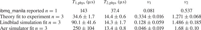
Figure 9. Numerical fits of several models to the data in figure 6 for the extreme conditions of localized (purple, $k=0.1$) and diffusive (red, $k=4.55$) dynamics. Models are described in the main text. Note that, for both values of $k$, the plots for the theory fit and Aer simulation fit overlap and resemble a solid line.

4.4 The IBM Aer gate-based Lindblad simulator

For artificial noisy simulators, IBM offers several options. One option is their device-specific noise models (IBM 2021a) that are calibrated to each device's reported errors. Reported $T_1$ and $T_2$ times and per gate error rates from RB are used as input for a combined relaxation, dephasing and depolarization error model. However, because these models are not customizable they cannot be fit to experimental data.

We instead use a custom IBM Aer noise model. Closest to our gate-based Linblad model is a simple Aer model based on the function thermal_relaxation_error with parameters $T_1$ and $T_2$ and an effective temperature that we set to zero (the default option) (IBM 2021c). This function applies a single-qubit Lindblad decay to each qubit targeted by a gate based on the duration of the gate, after the gate is done. When $T_2>T_1$, it applies Kraus operators, but when $T_2< T_1$, as is common, it probabilistically applies single-qubit gates instead. We modify this function to always apply Kraus operators. This model will be used in figure 9 to compare the relative importance of specifying the full gate dynamics as in Aer versus simplifying to the four unitary substeps (2.7) as in the gate-based Lindblad model.

4.5 Fitting theory to experiment

Having now described our noise models and performed derivations and simulations that qualitatively agree with experiment, it is interesting to fit these models to experiment to extract phenomenological decoherence parameters. The computational models can be fit through standard variational methods. The analytic gate-based Lindblad model from (4.14) has a fidelity that decays as

(4.18)\begin{equation} f_{\text{GB},S}(2 t_\text{fb} ) \approx \exp({-n_\text{eff} \nu_\text{single} * 2 t_\text{fb} }) (1-1/2^n) + 1/2^n, \end{equation}

where $n_\textrm {eff}=2$ for the two active qubits per gate, $t \equiv 2 t_\textrm {fb}$ with $t_\textrm {fb}$ as the number of forward-and-back pairs of map steps and $\nu _\textrm {single}$ depends on the dynamics of the map. After adjusting for the dynamics of the full QSM algorithm, the effect of localized dynamics is that

(4.19)\begin{equation} \nu_\text{single} = \nu_1/2 + \nu_2/8 = 3/8 T_1 + 1/4 T_2, \end{equation}

while the effect of diffusive dynamics is that

(4.20)\begin{equation} \nu_\text{single} = \nu_1/2+ \nu_2/4 = 1/4 T_1 + 1/2 T_2, \end{equation}

as explained in §§ 4.2 and 4.3, with further details in Appendix C.

To compare the experiment of figure 6 to this theory, it is convenient to focus on the extreme cases of $k=0.1$ and $k=4.55$. An account of continuously changing $k$ in a Lindblad model and its effect on fidelity would require a careful application of localization length to the Lindblad model, which is beyond the scope of this paper.

Figure 9 shows numerical fits to experimental fidelity of extreme $k$ for the gate-based Lindblad theory, the gate-based Lindblad simulations and an IBM-Q Aer simulator model, all described in § 4. Also included is the default Aer model from the function AerSimulator.from_backend(FakeManila()), which is designed to fit the error measured by RB.

The default Aer model underestimates error, but it only underestimates it by a factor of $1.5$ instead of $3.0{-}4.5$ from table 2. This is because it draws from a previous device calibration when the relevant gates were $2.0{-}3.0\times$ worse, artificially improving its accuracy. On average it is likely to be less accurate for the three-qubit QSM than shown here.

The three higher accuracy model fits demonstrate different approaches. The Lindblad theory fit uses the gate-based model (4.14) with rates (4.17) for localized dynamics and (4.12) for diffusive dynamics. The Lindblad simulation fit applies single-qubit relaxation and dephasing of uniform rates $\nu _1$ and $\nu _2$ continuously to two out of three qubits, alternating between qubits 0 and 1 or 1 and 2. This is applied during the four unitary steps per (2.7) evolved forward and back with QuTiP's mesolve function. The Aer simulator fit applies two-qubit and single-qubit gates followed by Kraus operators on the targeted qubits that are determined from decoherence parameters $T_{1,\textrm {phys}}$ and $T_{2,\textrm {phys}}$.

These models of fidelity all have just two parameters: $\nu _1$ for relaxation and $\nu _2$ for dephasing, which relate to the physical decoherence times through (4.7) and $T_1 = T_{1,\textrm {phys}}/T_\textrm {step}, T_2 = T_{2,\textrm {phys}}/T_\textrm {step}$. Here $T_\textrm {step}$ is the time to complete a single forward or backward map step on hardware, with $T_\textrm {step}=33*350 ns$ to match $33$ CNOT gates of average duration $\approx 350 ns$ on each of the forward-and-backward simulation steps. (This was an accurate average gate time when these experiments were performed, though since then IBM's two-qubit gates have changed in type and duration. (IBM 2022).) This only considers time spent in CNOT gates, in accordance with the single-gate-based Lindblad model. The Aer simulator model uses the same $T_\textrm {step}$ to convert between parameters, despite including single-qubit gates decaying at the same rate as the CNOT gates, since the single-qubit gates contribute $<5\,\%$ to the total duration of gates ($1/10$ the duration of a CNOT gate and $< 1/2$ as many gates). Since it directly fits $T_{1,\textrm {phys}}$ and $T_{2,\textrm {phys}}$, this extra error is in the converted $\nu _1$ and $\nu _2$ values. Measurement error is neglected in all models, which requires additional parameters to describe the probability of each state being misclassified, and which has a small effect on the large exponential decay rates measured here.

The fit of all three models in figure 9 is qualitatively quite good. The Lindblad simulation is a slightly worse fit than the others, which is surprising since it should be more accurate than the corresponding simplified theoretical model. The late time fit may appear to have higher error, but this is only an illusion of plotting the log of fidelity that accentuates the errors when the fidelity is small.

Table 3 provides the quantitative parameter fits. The most striking result is the consistent values of $T_2$ across models, as it is also the dominant error source. Here $T_2$ measures the dephasing of states that are in superposition, and the QSM with diffusive dynamics produces randomly entangled states that dephase similarly to superposition states (see Appendix C), so it is well suited to benchmark an effective version of this noise process. The agreement between models suggests the analytical model might be usable for lightweight extraction of the effective circuit $T_2$ time.

The variance across the fit $\nu _1$ and $\nu _2$ values suggests differing effective weights on each across the three models. The analytic model suggests that $\nu _2$ is the sole cause of a difference between localized and diffusive fidelity decay rates. However, three qubits is a small system and has poor random phase averaging for the diffusive case, which could alter the relative roles of $\nu _1$ and $\nu _2$. For larger system sizes, the simplified theoretical model should have better agreement with the simulation results.

The average $T_2$ fit of the three models is $14.0 \,\mathrm {\mu } \textrm {s}$, which is $2.7\times$ smaller than the reported single-qubit idle $T_2$ time from IBM-Q. It is no surprise that a complex circuit decoheres more quickly than idle qubits. The experimental $T_1$ fit values are less consistent, though this is due mostly to the small values of $\nu _1$ being close to zero and therefore being similar in magnitude to the error bars, making them difficult to resolve. In particular, the observed $T_1$ from the Aer simulator fit is larger than the reported idle value, casting some doubt on the model's accuracy with respect to $T_1$.

The ratio of idle $T_2$ to circuit CNOT $T_2$ is also a useful test of the question posed in Appendix A.1.2: How does the error of a CNOT gate $\epsilon _\textrm {CNOT}$ compare to the error of an idle gate of the same duration $\epsilon _\textrm {IDLE}$? This test is hampered somewhat by IBM-Q reporting a $T_2$ value measured by the Hahn echo $T_{2E}$. That experiment is less sensitive to ‘inhomogeneous broadening’, that is, low-frequency fluctuations that can cause large differences from trial to trial (Krantz et al. Reference Krantz, Kjaergaard, Yan, Orlando, Gustavsson and Oliver2019). Since $T_{2E} \ge T_2$, this only provides an upper bound, $\epsilon _\textrm {CNOT} / \epsilon _\textrm {IDLE} \lesssim T_{2E,\textrm {IDLE}} / T_{2,\textrm {CNOT}} \approx 3$, when the effective $T_1$ is negligible. This bound is right in between the limits of $\epsilon _\textrm {CNOT} = \epsilon _\textrm {IDLE}$ and $\epsilon _\textrm {CNOT} \gg \epsilon _\textrm {IDLE}$, suggesting that the benefit of gate parallelization must be treated carefully. In particular, the approximation of negligible idle error in § 4.3, which was reasonable to first order here, will become poor for serially executed circuits if even a few more idle qubits are added.