1. Introduction
The reliable prediction of the gas state at the surface of a hypersonic vehicle remains a unique challenge as hyper-velocity flows are strongly characterized by complex couplings between thermochemistry, transport phenomena and the fluid motion. At Mach numbers above 5 and depending on flight altitude, the gas surrounding the aircraft may locally depart from thermochemical equilibrium because time scales associated with fluid motion become comparable to those associated with internal energy relaxation and chemical reactivity (Anderson Reference Anderson2006). This generally requires finite-rate equations for internal energy relaxation and chemical reactions, together with a separate description of the average energy associated with each of the internal energy modes. The unique definition of a local thermodynamic temperature, or equivalently a partition function, becomes insufficient, as local energy distributions may deviate from equilibrium Boltzmann distributions. While relatively small, these deviations have a significant impact on finite-rate processes in the gas (Josyula, Bailey & Suchyta Reference Josyula, Bailey and Suchyta2011; Valentini et al. Reference Valentini, Schwartzentruber, Bender, Nompelis and Candler2015, Reference Valentini, Schwartzentruber, Bender and Candler2016; Grover et al. Reference Grover, Schwartzentruber, Varga and Truhlar2019a; Grover, Torres & Schwartzentruber Reference Grover, Torres and Schwartzentruber2019b; Torres & Schwartzentruber Reference Torres and Schwartzentruber2020; Torres, Geistfeld & Schwartzentruber Reference Torres, Geistfeld and Schwartzentruber2024). Moreover, the gas is also generally a mixture of molecular and atomic species and its composition cannot be obtained by assuming local thermodynamic equilibrium. Ultimately, the precise local state of the gas is determined by fundamental molecular-level interactions between atoms and molecules in the flow.
These physical considerations motivated the development of thermochemical non-equilibrium models based on a multi-temperature approximation. The local thermodynamic temperature of the gas is replaced by various temperatures corresponding to the average energy of each internal energy mode (rotational, vibrational and electronic). Then, the energy transfer between external and internal energy modes is described by relaxation-type equations, e.g. the Jeans equation for rotation (Jeans Reference Jeans2009) and the Landau–Teller equation for vibration (Landau & Teller Reference Landau and Teller1936). A common simplification of multi-temperature models reduces them to two-temperature descriptions (Park Reference Park1988) as, even at hypersonic conditions, rotational and translational modes for many diatomic gases are generally equilibrated throughout the flow, with the exception of shock interfaces and rapid expansions (Valentini et al. Reference Valentini, Grover, Bisek and Verhoff2021; Grover et al. Reference Grover, Verhoff, Valentini and Bisek2023b).
The success of these models largely relied on their clever description of thermal non-equilibrium (particularly vibrational non-equilibrium), their computational efficiency and ease of calibration against experimental (Park Reference Park1993) or first-principles (Chaudhry et al. Reference Chaudhry, Boyd, Torres, Schwartzentruber and Candler2020) data. Models calibrated with experimental evidence tend to have more limited predictive capability, as the calibration data are usually restricted to relatively low temperatures and are often characterized by significant uncertainty. In all cases, however, the formulation of multi-temperature models may be inherently too simplistic to account for the subtle, yet important, non-Boltzmann effects present in regions of the flow that are in strong thermochemical non-equilibrium (depleted vibrational energy distributions).
State-to-state (StS) models represent an accurate, but more computationally expensive, alternative to a multi-temperature description. In this framework, the distributions of molecules in every allowed molecular energy level are tracked by using a master equation (Fernández-Ramos et al. Reference Fernández-Ramos, Miller, Klippenstein and Truhlar2006; Capitelli et al. Reference Capitelli, Ferreira, Gordiets and Osipov2013) that requires transition rates between each and every internal molecular state. This approach, particularly when based on transition rate coefficients obtained from first principles (Panesi et al. Reference Panesi, Jaffe, Schwenke and Magin2013), removes any empiricism, but soon becomes computationally intractable for systems of more than three atoms, due to the extremely large number of transitions that must be accounted for with adequate statistical accuracy (Bender et al. Reference Bender, Valentini, Nompelis, Paukku, Varga, Truhlar, Schwartzentruber and Candler2015). Therefore, to reduce the computational cost, an order reduction is required, for example, by binning energy states together (Panesi et al. Reference Panesi, Magin, Bourdon, Bultel and Chazot2011; Guy, Bourdon & Perrin Reference Guy, Bourdon and Perrin2013; Liu et al. Reference Liu, Panesi, Sahai and Vinokur2015; Munafò, Liu & Panesi Reference Munafò, Liu and Panesi2015; Macdonald et al. Reference Macdonald, Jaffe, Schwenke and Panesi2018b). The resulting loss of accuracy from such simplifications should then be estimated via a comparison with results obtained without such biases (Macdonald et al. Reference Macdonald, Grover, Schwartzentruber and Panesi2018a).
Recently, several authors (Colonna, Bonelli & Pascazio Reference Colonna, Bonelli and Pascazio2019; Bonelli, Pascazio & Colonna Reference Bonelli, Pascazio and Colonna2021; Ninni et al. Reference Ninni, Bonelli, Colonna and Pascazio2022; Wang et al. Reference Wang, Guo, Hong and Li2023; Guo, Wang & Li Reference Guo, Wang and Li2024) have conducted computational fluid dynamics (CFD) studies of high-enthalpy flows using StS models for air species. In all cases, an order reduction was used, and the resulting StS models generally only account for certain vibration–vibration (VV) and vibration–translation (VT) transitions. All StS models were based on rates obtained from quasi-classical trajectory calculations conducted on disparate potential energy surfaces (PESs), from ab initio to semi-empirical. In all results, however, it was observed that the StS models provide better predictions for shock stand-off distances (Colonna et al. Reference Colonna, Bonelli and Pascazio2019; Guo et al. Reference Guo, Wang and Li2024) for air flows over spheres (Olejniczak et al. Reference Olejniczak, Candler, Wright, Leyva and Hornung1999; Nonaka et al. Reference Nonaka, Mizuno, Takayama and Park2000) compared with the results obtained from two-temperature models. Discrepancies in heat flux predictions between the StS and two-temperature models were also observed, with the former predicting a lower heat transfer rate (Guo et al. Reference Guo, Wang and Li2024). For some flows (Wang et al. Reference Wang, Guo, Hong and Li2023), such differences were shown to be relatively minor. The improved accuracy of StS models is attributed to their ability to describe non-equilibrium vibrational energy distributions throughout the flow (Colonna et al. Reference Colonna, Bonelli and Pascazio2019).
Although very powerful, the StS approach must still rely on various simplifications in order to be computationally feasible and applicable to production-level CFD codes. Furthermore, hypersonic conditions may also challenge the validity of certain constitutive relations, which are not affected by the choice of thermochemical models. In fact, transport coefficients are usually inconsistent with the PESs used to obtain the StS rate transition coefficients. For example, by using particle methods in the near-continuum regime (Grover et al. Reference Grover, Verhoff, Valentini and Bisek2023b; Valentini et al. Reference Valentini, Grover, Verhoff and Bisek2023), we observed that the Soret effect (Eastman Reference Eastman1928; Ferziger & Kaper Reference Ferziger and Kaper1993) may produce significant mass diffusion near the viscous wall in a hypersonic flow, which is characterized by strong temperature gradients near the aircraft surface. Contributions from thermal and pressure gradients are usually neglected in the mass diffusion flux in CFD codes utilized in engineering design (Wright, White & Mangini Reference Wright, White and Mangini2009). The mass transport effects in multi-component gas mixtures generated in the boundary layer of a reactive flow have important implications on gas–surface chemical interactions for both catalytic and ablative wall materials (Zibitsker et al. Reference Zibitsker, McQuaid, Stern, Palmer, Libben, Brehm and Martin2023) and for cold-wall-driven recombination (Gimelshein & Wysong Reference Gimelshein and Wysong2019).
In this work, we present the first direct molecular simulation (DMS) of a two-dimensional, reactive five-species ( ${\rm N}_2$,
  ${\rm O}_2$, NO, N and O) air flow over a blunt wedge at conditions where significant thermal and chemical non-equilibrium is observed in the shock layer.
The DMS method (Schwartzentruber, Grover & Valentini Reference Schwartzentruber, Grover and Valentini2018) is the ab initio variant of the well-known direct simulation Monte Carlo (DSMC) method of Bird (Reference Bird1994). The main difference between DMS and DSMC is that DMS does not utilize collision cross-section models for particle interactions. Instead, molecular dynamics (MD) trajectories are integrated on PESs specific to each molecular species pair in the gas mixture to obtain the mapping between initial (reactant) and final (product) states. Previously, it was shown that brute-force all-atom MD and DMS produce statistically identical results if both methods implement the same interaction potentials and the gas is at dilute enough conditions, i.e. particles interact only via collision-type events (Norman, Valentini & Schwartzentruber Reference Norman, Valentini and Schwartzentruber2013; Schwartzentruber et al. Reference Schwartzentruber, Grover and Valentini2018), and the assumption of molecular chaos is justified. The DMS method, however, is much more efficient than MD due to the decoupling of particles free flight from molecular interactions.
Each DMS particle undergoes a sequence of collisions while transiting in the flow domain or for the duration of the simulation while in the simulation box. The post-collision states are all the internal atomic coordinates (position and velocities in the centre of mass reference frame) and the centre of mass velocity at the end of each trajectory. For the next collision, these states become the initial conditions needed to time propagate the trajectory. The outcomes of each interaction are bound–bound transitions, bound–free transitions or exchange reactions. No electronic state changes are permitted, however, and thus the gaseous mixture remains in its electronic ground state, i.e. so-called five-species air. This enables a time-accurate gas flow simulation, where steady-state non-equilibrium molecular energy and velocity distributions may result in the flow (Valentini et al. Reference Valentini, Grover, Bisek and Verhoff2021; Grover et al. Reference Grover, Verhoff, Valentini and Bisek2023b). No decoupling or grouping of states is necessary because trajectories determine the state transition, without a priori restrictions, based on the local gas microscopic state and the PES on which the interaction occurs. This feature makes the DMS method essentially assumption free, and thus, DMS solutions have been used to benchmark reduced-order models, for example coarse-grained StS models (Macdonald et al. Reference Macdonald, Grover, Schwartzentruber and Panesi2018a), phenomenological DSMC (Valentini et al. Reference Valentini, Grover, Bisek and Verhoff2021) and, more recently, CFD multi-temperature models (Grover et al. Reference Grover, Verhoff, Valentini and Bisek2023b).
The DMS method is considerably more expensive than traditional DSMC, particularly when based on accurate ab initio PESs. For this reason, its application was initially restricted to simulate zero-dimensional reactors (Valentini et al. Reference Valentini, Schwartzentruber, Bender, Nompelis and Candler2015, Reference Valentini, Schwartzentruber, Bender and Candler2016; Grover et al. Reference Grover, Schwartzentruber, Varga and Truhlar2019a,Reference Grover, Torres and Schwartzentruberb) of single component systems (e.g.  ${\rm N}_2$ or
  ${\rm O}_2$). In recent years, thanks to advancements in large-scale computer technology, its application has been extended to zero-dimensional air reactors (Torres et al. Reference Torres, Geistfeld and Schwartzentruber2024), one-dimensional (Valentini et al. Reference Valentini, Grover, Bisek and Verhoff2021; Torres & Schwartzentruber Reference Torres and Schwartzentruber2022) and two-dimensional (Grover & Valentini Reference Grover and Valentini2021; Valentini et al. Reference Valentini, Grover, Bisek and Verhoff2021; Grover et al. Reference Grover, Valentini, Bisek and Verhoff2023a,Reference Grover, Verhoff, Valentini and Bisekb) single gas flows.
The work presented here represents a significant extension to full five-species air of our previous efforts aimed at obtaining the entire hypersonic aerothermodynamic field around a two-dimensional (or axisymmetric) body at near-continuum conditions. The objective of this effort is to derive an entire aerothermodynamic field from the fundamental description of how molecules and atoms interact at the microscopic level. This provides solutions where the coupling between the gas flow mechanics, the local gas-phase thermochemical non-equilibrium and the diffusive mechanisms for mass, momentum and energy are all obtained within a consistent, empiricism-free framework.
This article is organized as follows: we describe the DMS method in § 2. The PESs are listed in § 3. The details on the simulation set-up and parameters, boundary conditions and grid independence are presented in § 4. The results on the gas-phase thermochemistry and mass diffusion kinetics are discussed in § 5. Finally, the conclusions are contained in § 6.
2. Simulation method
The DMS method was originally devised as a way to combine the accuracy of MD trajectory integration with the efficiency of DSMC to simulate dilute gas flows (Matsumoto & Koura Reference Matsumoto and Koura1991; Koura Reference Koura1997, Reference Koura1998). As such, it was originally named as classical trajectory calculation (CTC) DSMC. Then, thanks to the significant improvements in computer technology over the years and with availability of new and accurate PESs for molecular interactions of air species, interest in its applications to high-temperature, reactive gas dynamics was renewed. The CTC DSMC was thus extended to molecules with internal degrees of freedom allowing for dissociation and exchange kinetics, and it was renamed DMS (Schwartzentruber et al. Reference Schwartzentruber, Grover and Valentini2018). We refer the reader to Schwartzentruber et al. (Reference Schwartzentruber, Grover and Valentini2018) for a detailed description of the method, together with the physical considerations associated with its implementation and with simulation parameter choices. Here, we will provide a brief overview for clarity of exposition.
Direct molecular simulation is a Lagrangian particle method, like DSMC. The gas is represented by particles that are advected based on their centre-of-mass velocity and collide with other molecules via collision-type interactions. The simulations are carried out with a time step of the order of the shortest mean collision time ( $\tau _c$) in the flow. The flow domain is subdivided into small control volumes (cells) whose size is of the order of the local mean free path (
 $\lambda _c$). Unlike pure MD, each control volume only contains a fraction of the total number of real molecules that would have been present based on the mass density in the cell. This is achieved by assigning a so-called particle weight
  $W_p$. The local collision frequency is obtained by the no-time counter (NTC) algorithm (Bird Reference Bird1994). In DMS, the collision cross-section is not known a priori, as it would be in standard DSMC (e.g. variable hard-sphere model). Instead, it is the PES that dictates the range of interaction within which the deflection angle is not negligible. As detailed by Schwartzentruber et al. (Reference Schwartzentruber, Grover and Valentini2018), this is achieved by utilizing a conservative hard-sphere (HS) cross-section
  $\sigma$ based on the imposed maximum collision parameter
  $b_{max}$, i.e.
  $\sigma ={\rm \pi} b_{max}^2$. In the simulation shown here,
  $b_{max}$ was initially set to 4 Å while the flow was establishing around the blunt wedge. Then, it was increased to a more conservative value of 6 Å during the flow-field sampling. The larger value was found to be adequate in several previous studies (Valentini et al. Reference Valentini, Schwartzentruber, Bender, Nompelis and Candler2015, Reference Valentini, Schwartzentruber, Bender and Candler2016; Grover & Valentini Reference Grover and Valentini2021; Torres & Schwartzentruber Reference Torres and Schwartzentruber2022; Grover et al. Reference Grover, Valentini, Bisek and Verhoff2023a,Reference Grover, Verhoff, Valentini and Bisekb). This approach was taken to minimize the time needed to establish a near-steady-state solution because the number of trajectories integrated at each time step scales as
  $b_{max}^2$. Once the sampling phase started, then
  $b_{max}$ was increased to its more conservative value.
Each DMS particle is internally structured as the real molecule it represents. Hence, the internal phase-space coordinates are consistent with its molecular structure (e.g. atomic, diatomic, triatomic, etc.). Trajectory propagation is obtained by integrating Newton's equation of motion using a finite difference, symplectic velocity-Verlet algorithm (Frenkel & Smit Reference Frenkel and Smit2002). Once again, in order to optimize the use of computer resources, the time step was set to 1 fs during the initial transient and it was decreased to a more conservative time step of 0.5 fs during the sampling of flow-field quantities. Note that the optimal time step needed to conserve total energy during each trajectory integration is a function of the local temperature. A further optimization, such as a cell-dependent MD time step used by Grover et al. (Reference Grover, Verhoff, Valentini and Bisek2023b), is possible but was not used in this study.
Trajectories are terminated when products are at a distance  $D_0$ that is large enough so that internal state changes can no longer occur. This separation
  $D_0$ is roughly
  $O(10 r_0)$, where, for air molecules, typical values of
  $r_0\simeq 1$ Å. For the results presented in this article,
  $D_0$ was set to a conservative value of 20 Å.
The stochastic parallel rarefied-gas time-accurate analyser (SPARTA) DSMC code (Plimpton et al. Reference Plimpton, Moore, Borner, Stagg, Koehler, Torczynski and Gallis2019) was modified to add the needed DMS capabilities. Trajectory integration was added as a new collide class. Function libraries implementing the Wentzel–Kramers–Brillouin method (Truhlar & Muckerman Reference Truhlar and Muckerman1979) were linked against the SPARTA code to provide product analysis (rotational and vibrational energies and numbers). Finally, particle internal data structures were augmented to accommodate for the internal phase-space coordinates. The current implementation supports up to two atoms per simulator particle (atomic or diatomic) and simple and double dissociations.
3. Potential energy surfaces
Direct molecular simulation calculations require interaction potentials between the various gas species in a mixture. For so-called five-species air, these species are  ${\rm N}_2$,
  ${\rm O}_2$, NO, N and O. Here, we only consider ground electronic states. For a chemically reacting air mixture, molecular collisions occur between two diatomic molecules (e.g.
  ${\rm N}_2+{\rm O}_2$), between a diatomic molecule and an atom (e.g.
  ${\rm NO}+{\rm O}$) or between two atoms (e.g.
  ${\rm O}+{\rm N}$). For isothermal zero-dimensional systems, typically referred to as chemical reactors, it is possible to exclude atom–atom interactions, as their only effect is to cause the very rapid translational relaxation of the atomic species, provided that no electronic excitation is included. For one- and two-dimensional flows, however, collisions involving atoms (either with other atoms or with the surface) must be included, as they play a fundamental role in momentum transfer that affects transport phenomena (e.g. mass diffusion, viscosity, etc.) and gas–wall interactions.
Although the DMS framework is independent of the PES choices, whether ab initio or semi-empirical (Grover et al. Reference Grover, Torres and Schwartzentruber2019b), in this work we only utilize ab initio surfaces, with two exceptions that will be discussed later. Therefore, within a first-principles description of ground-electronic-state air, each interaction may be described by multiple surfaces, which are the result of spin and spatial degeneracies. For example,  ${\rm O}_2+{\rm O}$ interactions are described by nine unique PESs, each with a precise statistical weight that essentially represents the fraction of trajectories that are integrated on that particular surface. Moreover, for certain interactions, in particular those with NO, coupling between ground-electronic-state reactants and electronically excited product states is possible. Those surfaces are not included in the present work (or even available in general) as we restrict DMS trajectories to ground electronic states without surface hopping. All ab initio PESs are found in Potlib (Shu et al. Reference Shu2023), an open-source repository maintained by the Theoretical and Computational Chemistry group at the University of Minnesota.
The work of Torres et al. (Reference Torres, Geistfeld and Schwartzentruber2024) discusses in detail available ab initio surfaces for air chemistry and their statistical weights. It is clear that, even for ground-electronic-state-only air, several PESs are still missing and will be hopefully calculated in the future. Notably, ab initio  ${\rm N}_2+{\rm NO}$ and
  ${\rm O}_2+{\rm NO}$ PESs are unavailable as of the writing of this article. The results presented here were obtained by selecting PESs and their corresponding statistical weights in the same manner as Torres et al. (Reference Torres, Geistfeld and Schwartzentruber2024). However, as explained by the same authors in an earlier article (Torres, Geistfeld & Schwartzentruber Reference Torres, Geistfeld and Schwartzentruber2023), other modelling choices are possible, for example by artificially rescaling the PESs weights in order to obtain a probability of one for an interaction to occur on a given available surface. For example, in our calculations, once a
  ${\rm NO}+{\rm NO}$ pair is selected to undergo a collision, the actual trajectory integration has a probability of 3/16 to occur, because the only available PES that can correctly describe the interaction is the
  ${\rm N}_2{\rm O}_2(1^3{\rm A})$ surface (Varga et al. Reference Varga, Meana-Pañeda, Song, Paukku and Truhlar2016), while the remaining surfaces are missing (Torres et al. Reference Torres, Geistfeld and Schwartzentruber2024).
As of the preparation of this article, we are not aware of a full ab initio treatment for  ${\rm N}_2+{\rm NO}$ and
  ${\rm O}_2+{\rm NO}$ interactions. For air chemistry in a box, the reactions caused by collisions between NO and
  ${\rm N}_2$ or NO and
  ${\rm O}_2$ were recognized to be of secondary importance (Torres et al. Reference Torres, Geistfeld and Schwartzentruber2024), as the kinetics of NO production were largely attributed to Zeldovich reactions. In particular, the main reaction responsible for generating NO is the first Zeldovich reaction
  ${\rm N}_2+{\rm O}\rightarrow {\rm NO}+{\rm N}$, due to readily available oxygen atoms produced by the dissociation of molecular oxygen. In fact, even at only moderately high Mach numbers,
  ${\rm O}_2$ dissociates in larger quantities than
  ${\rm N}_2$ due to its weaker molecular bond. At shock layer temperatures as high as 10 000 K, nearly no oxygen remains in a molecular form (Grover et al. Reference Grover, Torres and Schwartzentruber2019b), whereas only incipient molecular nitrogen dissociation is observed (Valentini et al. Reference Valentini, Schwartzentruber, Bender, Nompelis and Candler2015). Therefore, with the exception of very high Mach regimes, for example for planetary entry, the mass fraction of molecular nitrogen would be quite close to the free-stream value, whereas abundant atomic oxygen would be present. Inevitably, collisions between O and
  ${\rm N}_2$ would produce a significant amount of NO, which in turn would readily collide with the similarly abundant
  ${\rm N}_2$. Hence,
  ${\rm N}_2+{\rm NO}$ and, to a lesser extent,
  ${\rm O}_2+{\rm NO}$ collisions are expected to be important as far as mass, momentum and energy diffusion mechanisms are concerned. For this reason, we decided to use semi-empirical surfaces for these interactions (Andrienko & Boyd Reference Andrienko and Boyd2018). Although these PESs were not obtained from first principles, they surfaces were built using sound physical considerations. In our implementation, for simplicity, we removed energy contributions from dipole–dipole and dipole–quadrupole interactions as they are negligible at the high temperatures characteristic of hypersonic flight (Andrienko & Boyd Reference Andrienko and Boyd2018). The diatomic energies for NO,
  ${\rm N}_2$ and
  ${\rm O}_2$ had to be slightly corrected (energy-well depth) in order to ensure consistency with the remaining ab initio PESs. The
  ${\rm N}_2+{\rm NO}$ and
  ${\rm O}_2+{\rm NO}$ surfaces have a simple analytic form. Nonetheless, they were shown to well-reproduce NO vibrational relaxation times and provide reasonable results for NO dissociation.
Three-atom products, such as  ${\rm N}_2{\rm O}$ or
  ${\rm NO}_2$ were sporadically recorded from trajectories on the
  ${\rm N}_2{\rm O}_2(1^3{\rm A})$ surface (Varga et al. Reference Varga, Meana-Pañeda, Song, Paukku and Truhlar2016). We estimated, however, that they represented approximately
  $1\times 10^{-5}$ % of all integrated collisions during the sampling window. Therefore, it is not expected that these trajectories influence the overall computation. When detected at the end of a trajectory, the particles’ phase-space coordinates were reset to the initial conditions, i.e. the entire trajectory was ignored.
Finally, although the DMS method is essentially assumption free, the inclusion of recombination mechanisms remains a challenge. Another significant challenge is the simulation of electronic excitation, which presents its own unique set of difficulties related to the large number of electronically excited surfaces and their couplings as well as the need for non-adiabatic trajectory integration. Therefore, neither recombination nor electronic excitation are included here.
A summary of the PESs used in this work is contained in table 1 with the corresponding references. For each interaction, we list whether the set of ab initio PESs is incomplete. Note that for some of the listed PESs, neural network fits were also provided in Potlib (Shu et al. Reference Shu2023). In this work, however, all PESs were based on permutation-invariant polynomial fits.
Table 1. Interaction potentials (PESs) between air particles and corresponding references. The asterisk ( $^*$) denotes a semi-empirical surrogate PES.

3.1. Calculation of internal energies and definition of macroscopic temperature
In the DMS method, the independent variables that uniquely describe the molecular state for each  ${\rm N}_2$,
  ${\rm O}_2$ and NO molecule are the atomic position and velocities of the constituting atoms. The translational energy associated with the motion of the centre of mass is usually referred to as an external energy mode. The positions and velocities in the centre-of-mass reference frame are associated with internal energy modes. For molecules in the electronic ground state, the total energy is usually partitioned into translational (external), and rotational and vibrational (internal) contributions. In quantum mechanics, the molecular internal energy
  $\varepsilon _{int}(j,v)$ is usually expressed as a function of its rotational and vibrational numbers. For classical molecules,
  $j$ and
  $v$ represent the classical analogues obtained from the Wentzel–Kramers–Brillouin semi-classical method (Truhlar & Muckerman Reference Truhlar and Muckerman1979). For classical degrees of freedom, however,
  $\varepsilon _{int}(j,v)$ cannot simply be expressed by a sum of
  $\varepsilon _{rot}(j)$ (rotational energy) and
  $\varepsilon _{vib}(v)$ (vibrational energy). In fact, the separation of internal energy into its rotational and vibrational quotas is essentially arbitrary, as discussed in detail by Bender et al. (Reference Bender, Valentini, Nompelis, Paukku, Varga, Truhlar, Schwartzentruber and Candler2015), Panesi et al. (Reference Panesi, Jaffe, Schwenke and Magin2013) and Grover et al. (Reference Grover, Verhoff, Valentini and Bisek2023b). Following an established convention (Panesi et al. Reference Panesi, Jaffe, Schwenke and Magin2013; Torres & Schwartzentruber Reference Torres and Schwartzentruber2020, Reference Torres and Schwartzentruber2022; Grover et al. Reference Grover, Verhoff, Valentini and Bisek2023b), we adopted a so-called vibration-prioritized splitting of internal energy, where the vibrational energy is defined as
 \begin{equation} \varepsilon_{vib}(v) = \varepsilon_{int}(j=0,v), \end{equation}
and
 \begin{equation} \varepsilon_{rot}(j) = \varepsilon_{int}(j,v) - \varepsilon_{vib}(v). \end{equation}
As discussed by Torres & Schwartzentruber (Reference Torres and Schwartzentruber2020), with the exception of translational energy, it is problematic to compute the macroscopic temperature associated with internal energies from the average molecular energies
 \begin{equation} \tilde{T}_{rot,vib} = \frac{\langle \varepsilon_{rot,vib} \rangle}{k_B}, \end{equation}
where  $k_B$ is Boltzmann's constant and
  $\tilde {T}_{rot,vib}$ represent the temperatures associated with the rotational and vibrational energies possessed on average by the molecules in the flow. Clearly, under thermodynamic equilibrium, a unique temperature
  $T$ can be defined, with
  $T=T_{tra}=T_{rot}=T_{vib}$. This is because, in the thermodynamic limit, the temperatures expressed by (3.3) do not coincide with the temperature that uniquely defines the partition function obtained with the energy eigenstates. Torres & Schwartzentruber (Reference Torres and Schwartzentruber2020) and Panesi et al. (Reference Panesi, Jaffe, Schwenke and Magin2013) discuss how a better definition for
  $T_{rot,vib}$ should be obtained by determining the temperature from the computed distribution functions in each simulation cell. This approach is feasible for zero-dimensional reactors or StS methods, but becomes impractical for simulations containing thousands to millions of cells.
In this work, we follow the same approach as Grover et al. (Reference Grover, Verhoff, Valentini and Bisek2023b) by using a simple functional polynomial fit for  $T_{rot,vib}$
 \begin{equation} T_{rot,vib} = \sum_{i=0}^{3} a_i \left(\frac{ \tilde{T}_{rot,vib} }{20\,000\ \text{K}} \right)^i. \end{equation}
Here, we choose a third-order polynomial function. Figure 1 shows the average rotational and translational energies, rescaled with  $k_B$, as a function of the equilibrium temperature
  $T_{rot,vib}$. First, it can be seen that the rotational temperature is well approximated by
  $\tilde {T}_{rot}$. For the vibrational temperature, however,
  $\tilde {T}_{vib}$ generally overestimates the partition function based thermodynamic temperature, particularly at high temperatures. This behaviour is attributed to the anharmonic functional form of the diatomic energy curve, as previously discussed by Valentini et al. (Reference Valentini, Norman, Zhang and Schwartzentruber2014) within the context of empirical Morse-like potential energy curves. The fitting parameters
  $a_i$ are listed in table 2 for a temperature range between 100 and 20 000 K. It is important to emphasize that the fits are applied to the results obtained from the DMS computations as an independent post-processing step. They do not enter the DMS computations as input or assumption.

Figure 1. Variation of average rotational and vibrational energy as a function of temperature for (a)  ${\rm N}_2$, (b)
  ${\rm O}_2$ and (c) NO.
Table 2. Fitting parameters for the polynomial dependence in (3.4) of temperature on average rotational and vibrational energies.

4. Simulation details
A Mach 15 air flow over a blunt two-dimensional wedge is presented in this work. The free-stream conditions are listed in table 3. The blunt wedge has a leading edge radius of 1 cm, a half-angle of  $15^\circ$ and a total length of 5 cm. A schematic of the geometry and boundary conditions is shown in figure 2. Particles were injected into the flow domain across a parabolic inflow surface. This was done to minimize the extent of the free-stream region to reduce the computational resources required to carry out the simulation. The inflow surface was tailored with a DSMC simulation to be conservative enough so that it would not interfere with the bow shock that forms around the blunt wedge. The simulation domain box was likewise sized so that the bow shock would not impinge on the upper specular wall. The outflow boundary conditions was set as supersonic, i.e. without back pressure. This is fully justified by the inviscid surface wall.
Table 3. Free-stream conditions for the Mach 15 air flow over a blunt two-dimensional wedge.

Figure 2. Schematics of the wedge geometry and boundary conditions.
In previous works (Grover et al. Reference Grover, Valentini, Bisek and Verhoff2023a,Reference Grover, Verhoff, Valentini and Bisekb), we imposed a viscous wall boundary condition by assigning it a fixed temperature (isothermal wall) and considering full thermal and momentum accommodation for particles impinging on it. Because of the complexity associated with the multi-species simulation presented here, and in order to isolate gas-phase thermochemical kinetic mechanisms, we decided to model the wedge as inviscid. Therefore, particles impinging on the wedge surface are specularly reflected and their internal energies remain unchanged. This is not an inherent limitation of the DMS method and future work will include viscous wall effects.
Finally, based on the free-stream mean free path, we estimated a Knudsen number of  ${\sim }10^{-3}$ based on the wedge leading edge radius. Considering the density jump across the bow shock, this flow can be considered at near-continuum conditions in the shock layer.
4.1. Grid-independence study
The SPARTA code provides adaptive mesh refinement procedures that are needed to refine the Cartesian mesh in regions of high density. This is particularly advantageous in DSMC because of the requirement to resolve the local mean free path (Bird Reference Bird1994). A uniform grid able to resolve the smallest mean free path in the entire flow would inevitably result in an unnecessarily large number of cells. This is not optimal from a computational perspective. In addition, the number of particles would become unnecessarily large in order to have at least  ${\sim }20$ particles in each collision cell.
In the simulation presented here, Cartesian cells were progressively split in half in both the  $x$ and
  $y$ directions. Hence, a cell selected for refinement was subdivided in four child cells. The refinement criterion used the cell-based Knudsen number
  $Kn_c$
 \begin{equation} Kn_c = \frac{\lambda_{HS}}{\delta_c}, \end{equation}
where  $\lambda _{HS}$ is the mean free path based on the HS model and
  $\delta _c$ the cell size. The refinement condition was then set to
  $Kn_c > 1$, which implies that
  $\delta _c<\lambda _{HS}$. The resulting mesh exhibited progressive refinement in the shock layer toward the wedge surface because of the rise in mass density due to the compression of the air flow.
A typical rule of thumb in DSMC is to obtain a  $Kn_c > 1$ and
  ${\sim }20$ particles in each collision cell. As discussed before, however, the true mean free path
  $\lambda$ is not known (or even well defined) a priori in DMS. Because the HS model used in the NTC algorithm is equipped with a conservatively large collision cross-section (or, equivalently, constant impact parameter
  $b_0$), the satisfaction of the criterion expressed by (4.1) could result in an excessively fine mesh. Therefore, in order to reduce to a minimum the overall computational cost of the simulation, the maximum number of refinement levels (i.e. the maximum number of times a cell was eligible for refinement) was held fixed to four levels until steady state. The initial Cartesian mesh was sized such that the free-stream
  $Kn_c\simeq 1$. The NTC time step was set to 2 ns, approximately 1/5 the smallest mean collision time occurring in the vicinity of the stagnation point. After sampling the solution for 1500 time steps with samples collected at each time step, the maximum number of refinement levels was increased to five and the solution advanced for another 3000 time steps, with samples collected in the last 500 steps.
Using this procedure, we compared the solution obtained on both the 4-level (coarse) and on the 5-level (fine) grid systems. Both the coarse and fine grids contained approximately 420 million particles, resulting in approximately 85 million trajectories per time step and approximately a total of 260 billion integrated trajectories during the sampling window. The total number of cells in the coarse and fine grid systems were approximately 10 and 18 million, respectively. The number of particles per cell varied between approximately 14 and 50 in the fine grid system. The simulation was carried out using 7488 cores and required a total of about 6 million CPU hours on an HPC system equipped with AMD 9654 Genoa ${\circledR}$ 2.1 GHz processors.
In figures 3(a)–3(d), we plot various isolines for the temperatures (translational  $T_{tra}$, rotational
  $T_{rot}$ and vibrational
  $T_{vib}$), and the magnitude of the flow velocity (
 $|\boldsymbol {u}|$) for the overall air mixture. Data are shown for the coarse and fine grid systems in the region of the shock layer surrounding the stagnation point, i.e. a critical region of the flow. The resulting flow-field solutions are nearly overlapping. Furthermore, we extracted data along the stagnation line. The flow profiles are shown in figures 4(a)–4(e). For all species, partial density profiles are nearly identical on the two grid systems. For
  ${\rm N}_2$ and
  ${\rm O}_2$, temperature profiles show negligible differences. For species that are produced by dissociation or exchange reactions (NO, N and O), temperatures tend to fluctuate wildly in the upstream region of the shock, where their mass densities are very small. Therefore, these fluctuations are attributable to statistical noise. However, once significant amounts of these product species are present in the flow, their temperature profiles obtained on the coarse and fine grid are aligned. To conclude, we considered the solution obtained using the fine Cartesian mesh as grid independent. All results presented in the following were obtained on the fine grid system.

Figure 3. Comparison between coarse and fine grid isolines for (a) flow speed, (b) translational  $T_{tra}$, (c) rotational
  $T_{rot}$, (d) vibrational
  $T_{vib}$ temperature in the vicinity of the stagnation point.

Figure 4. Comparison between stagnation line profiles for all air species obtained on the coarse and fine grid systems.
5. Results
5.1. Shock layer thermal and chemical state
An overview of the flow field is shown in figure 5 where the Mach number across the simulation domain is shown. The Mach 15 air flow is compressed by the blunt wedge, resulting in the formation of a bow shock. The region surrounding the stagnation point is subsonic (the dashed line marks the sonic condition), and most of the flow remains supersonic along the wedge, as there is no viscous wall to cause the gas to slow down near the wedge surface.

Figure 5. Mach number across the simulation domain.
In figures 6(a)–6(d), we show several flow-field quantities of interest obtained from the DMS computation, with the data obtained for the overall gas mixture. As shown in figure 6(a), the shock layer translational temperature reaches approximately 14 000 K in the near-normal shock formed at the leading edge of the blunt wedge and then decays to plateau at approximately 8000 K along the stagnation line. The very high translational temperature reached in the vicinity of the stagnation point is responsible for most of the chemical dissociation observed in the flow and discussed later. Figures 6(b)–6(c) show the internal temperatures  $T_{rot}$ and
  $T_{vib}$. These were obtained from the corresponding internal energies averaged over the diatomic particles in each computational cell. The polynomial correction (3.4) was then applied with the fitting parameters listed in table 2. The rotational energy mode is seen to excite at a much faster rate than the vibrational energy mode, which reaches
  ${\simeq }8000$ K only near the stagnation point. For completeness, figure 6(d) shows the total mass density across the flow domain. The highest mass density is found in the stagnation point region.

Figure 6. Air mixture (a) translational, (b) rotational and (c) vibrational temperature, and (d) total mass density across the flow domain.
Similar to Grover et al. (Reference Grover, Verhoff, Valentini and Bisek2023b), we define a thermal non-equilibrium parameter
 \begin{equation} \eta_{rot,vib} = \frac{T_{tra}-T_{rot,vib}}{T_{tra}}, \end{equation}
which reduces to zero under local thermal equilibrium. Figures 7(a)–7(c) and 8(a)–8(c) show  $\eta _{rot}$ and
  $\eta _{vib}$, respectively, for each of the molecular species present in the flow. Rotational non-equilibrium, indicated by
  $\eta _{rot}\ne 0$, is essentially confined to the bow shock internal structure for both molecular nitrogen and oxygen. Nitric oxide is not present in the free stream, but it starts forming near the shock interface, where
  $\eta _{rot}<0$. This implies that
  $T_{tra}< T_{rot}$ slightly ahead of the shock. Thus, NO forms rotationally hot, as will be further discussed later. Its equilibration with the translational modes is then very quick, and the computation shows that
  $\eta _{rot}\simeq 0$ nearly throughout the shock layer.

Figure 7. Rotational thermal non-equilibrium parameter (5.1) for (a)  ${\rm N}_2$, (b)
  ${\rm O}_2$ and (c) NO across the flow domain in the region surrounding the stagnation point.

Figure 8. Vibrational thermal non-equilibrium parameter (5.1) for (a)  ${\rm N}_2$, (b)
  ${\rm O}_2$ and (c) NO across the flow domain in the region surrounding the stagnation point.
Vibrational non-equilibrium is, instead, much more pronounced throughout the shock layer. This is especially visible for molecular nitrogen in figure 8(a). This behaviour is less pronounced for  ${\rm O}_2$ due its relatively faster vibrational relaxation time compared with
  ${\rm N}_2$ at the temperatures reached in the shock layer. On the other hand, the NO vibrational non-equilibrium parameter
  $\eta _{vib}$ is remarkably similar to its rotational non-equilibrium one. In fact, similar to the rotational mode, the NO vibrational energy mode is initially characterized by
  $\eta _{vib}<0$, which indicates production of vibrationally hot nitric oxide. Notably, the subsequent equilibration with the translational energy modes is very rapid and
  $\eta _{vib}$ is nearly zero across the majority of the shock layer.
Near the junction between the rounded nose and the flat wall  $\eta _{vib}<1$ and remains negative along the flat wedge surface. This is indicative of a rapid expansion that produces a vibrationally frozen flow along the wedge surface, where
  $\eta _{vib}$ remains negative. Because the wall is modelled as inviscid, there is no further mechanism to generate a temperature variation along the wall normal, and the frozen flow is advected toward the supersonic outlet.
The flow remains at near-continuum conditions nearly throughout the domain, as evidenced by the density-based gradient-length local Knudsen number ( $Kn_{GLL}$) investigated by Wang & Boyd (Reference Wang and Boyd2003) to analyse the continuum breakdown. This parameter is defined as
 \begin{equation} Kn_{GLL} = |\boldsymbol{\nabla} \rho| \frac{\lambda}{\rho}. \end{equation}
For high-speed flows, Wang & Boyd (Reference Wang and Boyd2003) found that  $Kn_{GLL} > 0.05$ generally indicates a break down of the continuum regime. From figure 9, it is clear that
  $Kn_{GLL}$ remains well below 0.05 throughout the flow field, with the exception of the shock front.

Figure 9. Density-based gradient-length local Knudsen number across the flow domain.
The chemical activity in the flow is shown in figures 10, 11 and 12. Both molecular oxygen and nitrogen undergo significant dissociation in the hot shock layer near the stagnation point. Upon comparing figure 10 with figure 11, it is evident that  ${\rm O}_2$ nearly completely dissociates, whereas
  ${\rm N}_2$ dissociation is more modest. The concentration of atomic oxygen reaches approximately
  ${\sim }13$ % by mass fraction, as shown in figure 11(b). The relative abundance of O atoms and
  ${\rm N}_2$ molecules is the cause for the formation of NO seen in figure 12. The first Zeldovich reaction
  ${\rm N}_2+{\rm O}\rightarrow {\rm NO}+{\rm N}$ is likely to be primarily responsible for the NO formation in the vicinity of the stagnation point. The second Zeldovich reaction
  ${\rm O}_2+{\rm N}\rightarrow {\rm NO}+{\rm O}$ is likely to be secondary, as the availability of molecular oxygen quickly reduces along the stagnation streamline, whereas the availability of atomic nitrogen is limited. Nonetheless, both reactions are likely to take place in the DMS simulation, albeit at reactant-limited speeds. The concentration of nitric oxide peaks at
  ${\sim }1$ mm from the stagnation point, where it reaches approximately
  ${\sim }14$ % by mass fraction. Then, it decreases by approximately 40 % due to its dissociation as well, which is likely to result in additional N formation that accumulates near the stagnation point at the wall (figure 10), reaching concentrations around 2 %–3 %.
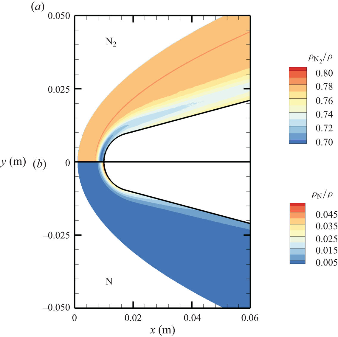
Figure 10. Mass fractions for  ${\rm N}_2$ (a) and N (b) across the flow domain.
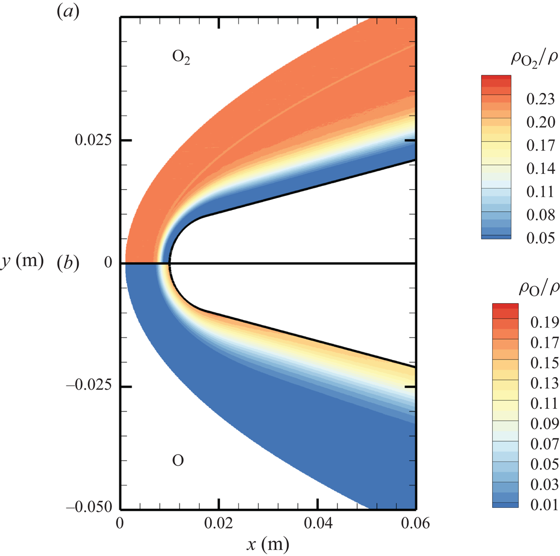
Figure 11. Mass fractions for  ${\rm O}_2$ (a) and O (b) across the flow domain.
Figure 12. Mass fractions for NO across the flow domain.
The precise chemical state of the gas in the shock layer surrounding a hypersonic vehicle has multiple important implications. First, it determines the heat flux that the thermal protection system has to withstand. Second, NO is a strong radiator. Third, atomic nitrogen has a significantly higher Gladstone–Dale constant and thus, its presence markedly affects the optical properties of the shock layer. Hence, it is of paramount importance to have reliable thermochemical models capable of accurately predicting the non-equilibrium chemical state of the high-temperature air mixture around a hypersonic aircraft.
The stagnation streamline profiles for various flow quantities are shown in figures 13(a)–13(d). For molecular nitrogen and oxygen, translational, rotational and vibrational temperatures display similar trends, consistent with previous DMS studies on one- and two-dimensional flows characterized by the presence of a (near-)normal shock wave and based on the same PESs that are used in this work (Valentini et al. Reference Valentini, Grover, Bisek and Verhoff2021; Torres & Schwartzentruber Reference Torres and Schwartzentruber2022; Grover et al. Reference Grover, Verhoff, Valentini and Bisek2023b). By comparing figure 13(a) with figure 13(b), the much slower vibrational relaxation time for  ${\rm N}_2$ can be clearly observed. The vibrational temperature of oxygen approaches the rotational and translational temperatures more slowly, but does not fully equilibrate with them. This is indicative of a so-called quasi-steady state (QSS) produced by the significant dissociation that
  ${\rm O}_2$ undergoes as it approaches the wall at the stagnation point. This feature is the result of the strong coupling between vibrational energy relaxation and vibrational energy removal due to dissociation, as extensively discussed in many previous works (Valentini et al. Reference Valentini, Schwartzentruber, Bender, Nompelis and Candler2015; Grover et al. Reference Grover, Torres and Schwartzentruber2019b; Torres et al. Reference Torres, Geistfeld and Schwartzentruber2024).
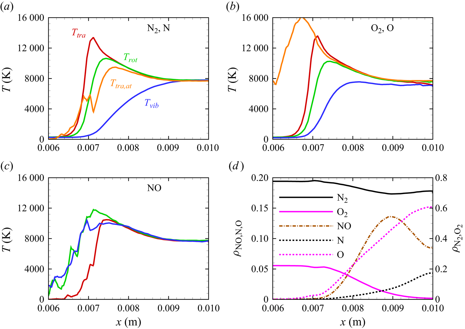
Figure 13. Stagnation streamline profiles for temperatures of (a)  ${\rm N}_2$ and N, (b)
  ${\rm O}_2$ and O, (c) NO; (d) profiles for mass fractions.
The production of atomic nitrogen and oxygen is evidenced by their translational energy profiles shown in figures 13(a)–13(b). The computation indicates a fast equilibration with the external modes of the molecular species as expected. However, atomic oxygen reaches much higher temperatures than nitrogen. Although the statistics of the upstream portion of the atomic profiles are generally poor, due to the relatively small concentration of atomic species, the difference could be attributed to the location at which significant dissociation starts occurring. In fact, for atomic oxygen, the dissociation process becomes quite significant more upstream than for atomic nitrogen, where translational and internal energies of the molecular species are generally larger and the gas mixture is less dense. Hence, the thus formed oxygen atoms collide in a much more energetic environment compared with nitrogen atoms, but their collision frequency is also smaller due to the lower density in the gas, which delays their thermal equilibration. Moreover, only two of the three surfaces for  ${\rm N}_2+{\rm O}$ interactions are available, whereas the full set of three surfaces was used for
  ${\rm O}_2+{\rm N}$. In practice, one third of the
  ${\rm N}_2+{\rm O}$ collision does not occur in the region where O is formed at the onset of the near-normal shock. This is likely to produce a more marked diffusion of O atoms upstream and, due to the artificially lower collision frequency, a delayed equilibration of the O atoms.
In figure 13(c), we show the NO temperature profiles. The formation of NO in the shock layer begins as soon as atomic oxygen becomes available due to  ${\rm O}_2$ dissociation. As previously discussed, atomic oxygen readily reacts with the abundant molecular nitrogen via the first Zeldovich reaction
  ${\rm N}_2+{\rm O}\rightarrow {\rm NO}+{\rm N}$. This behaviour was also observed in zero-dimensional chemical reactors studied by Torres et al. (Reference Torres, Geistfeld and Schwartzentruber2024) using the same set of PESs. The newly formed nitric oxide is rotationally and vibrationally hot. This behaviour was also observed by Torres et al. (Reference Torres, Geistfeld and Schwartzentruber2024) in zero-dimensional systems. Furthermore, the average internal energies in rotational and vibrational modes are nearly equilibrated as soon as NO is generated. As it is an exchange reaction that is responsible for the production of NO, products have no memory of any initial state and thus are more subjected to energy scrambling, as was observed in the case of
  ${\rm N}_2+{\rm N}$ exchange mechanisms (Valentini et al. Reference Valentini, Schwartzentruber, Bender and Candler2016). Further downstream, NO is essentially in thermal equilibrium
  $T_{tra}=T_{rot}=T_{vib}$.
Figure 13(d) shows the gas composition along the stagnation line. At these flow conditions, molecular oxygen is nearly depleted by the stagnation point, where the air mixture contains approximately 15 % atomic oxygen by mass fraction. Molecular nitrogen shows a much more modest reduction instead. The NO concentration steadily increases to peak at  $x\simeq 0.009$ m reaching approximately 14 % by mass fraction, then it decreases likely due to dissociation and other exchange processes. As stated in § 3, no recombination occurs. Therefore, the chemical composition is driven by either dissociation (simple or double) or exchange mechanisms.
As indicated by  $T_{vib}>T_{tra}$ (
 $\eta _{vib}<0$) and
  $T_{rot}>T_{tra}$ (
 $\eta _{rot}<0$) after the nose shoulder, the flow remains frozen, largely vibrationally, due to the expansion. This is more clearly illustrated by the flow profiles extracted along lines orthogonal to the wedge surface at
  $x_1 = 0.02$ m and
  $x_2 = 0.05$ m, shown in figures 14(a)–14(b), 15(a)–15(b) and 16(a)–16(b). Similarly to the stagnation line profiles, the slower vibrational relaxation time for
  ${\rm N}_2$ results in a larger difference between
  $T_{tra}$ and
  $T_{vib}$ near the inviscid wall as compared with
  ${\rm O}_2$ and NO. For all molecular species, rotational non-equilibrium is of secondary importance.
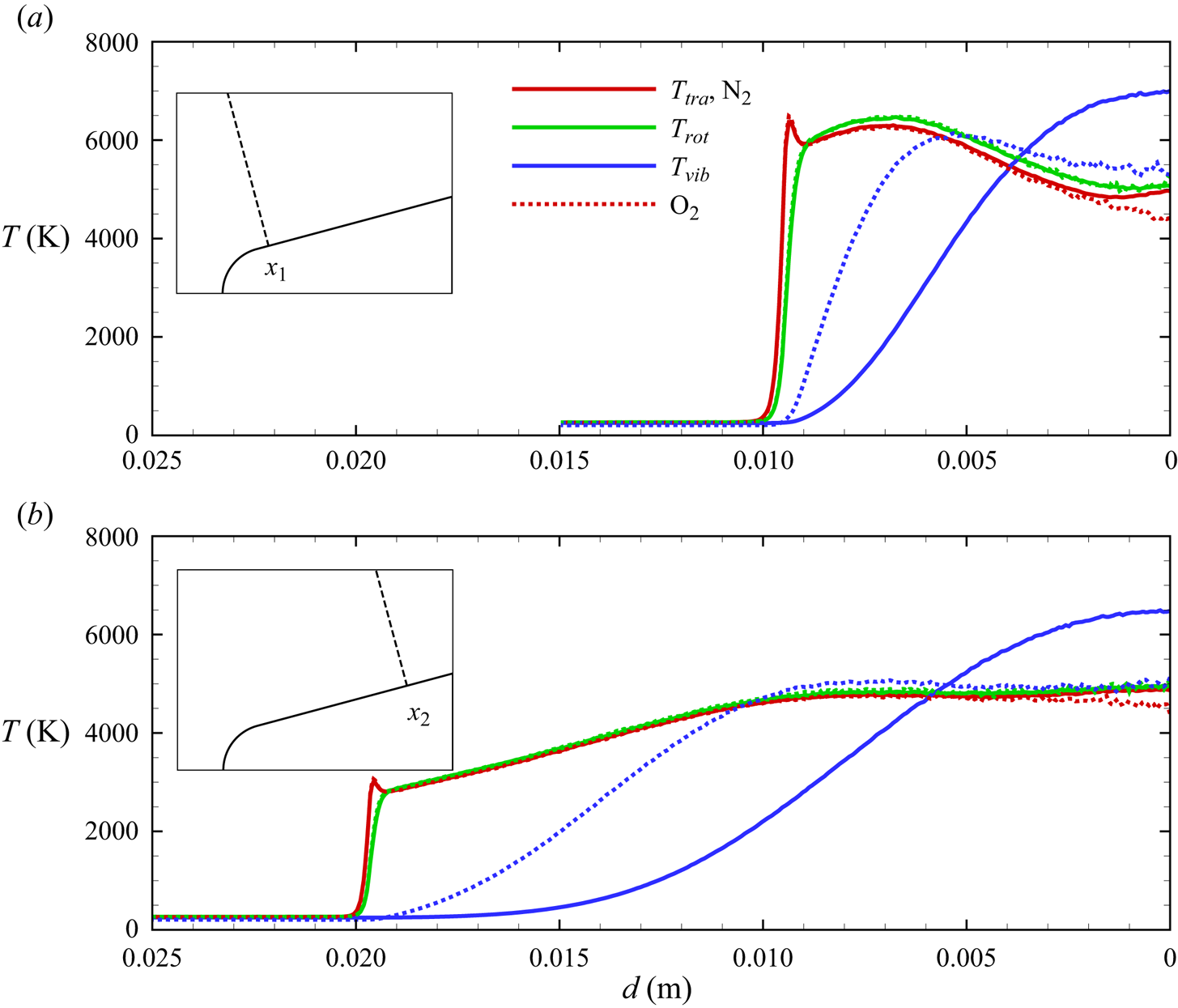
Figure 14. Molecular nitrogen and oxygen temperature profiles along extraction lines orthogonal to the wedge surface.

Figure 15. The NO temperature profiles along extraction lines orthogonal to the wedge surface.
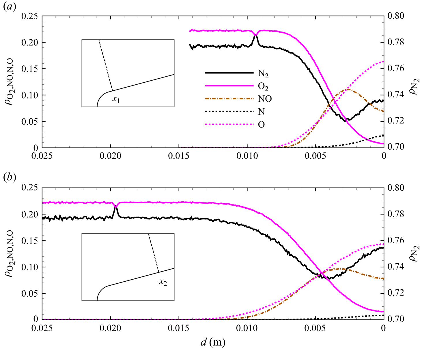
Figure 16. Mass fraction profiles along extraction lines orthogonal to the wedge surface.
As no friction is present at the surface, the flow advects toward the outlet and its structure remains qualitatively similar along the wedge. A notable feature is the mass fraction variation for  ${\rm N}_2$ and
  ${\rm O}_2$ at the oblique shock front, observed at
  $d\simeq 0.01$ m in the profile extracted at
  $x_1=0.01$ m, and similarly for the profile at
  $x_2=0.05$ m (
 $d\simeq 0.02$ m). The
  ${\rm N}_2$ mass fraction shows a local peak that corresponds to a dip in O
 $_2$ mass fraction. We attribute this phenomenon to multi-component diffusion mechanisms driven by the strong temperature (Soret effect) and pressure (barodiffusion) gradients (Ferziger & Kaper Reference Ferziger and Kaper1993) that characterize the shock wave structure, as discussed in § 5.3.
Finally, figure 17 reports the wall pressure on the wedge surface. The maximum pressure reaches approximately 23 000 Pa at the stagnation point, then rapidly decreases around the circular leading edge. The wall pressure along the flat portion of the wedge remains relatively constant at approximately 3000 Pa, with a slight decrease as the gas advects towards the supersonic outflow. As no viscous interactions with the wall are modelled in the present study, the surface heat flux is zero as the wall is adiabatic. This modelling choice was made to precisely isolate gas-phase chemistry phenomena only. In a later work, we will address the effect of gas–wall viscous interactions, the resulting boundary layer thickness and the related diffusion mechanisms.

Figure 17. Pressure distribution along the wedge's surface.
5.2. Local velocity and energy distributions
Particle methods, like DMS, allow the extraction of molecular-level information at any location in the flow field. Because each DMS particle stores internal energies, distributions for both rotational and vibrational energies can be obtained for each species of the air mixture. Clearly, atomic species can only be characterized by their velocity distributions if no electronically excited states are considered.
In figures 18(a)–18(e) and 19(a)–19(e), we plot molecular oxygen distributions obtained at two locations along the stagnation streamline. Figure 18(b–e) shows probability densities for oxygen molecules at  $x=0.007$ m, i.e. at a location nearly within the shock front. A total of nearly 200 000
  ${\rm O}_2$ molecules were collected over 2000 time steps at intervals of 5 time steps in a region
  $x\in [0.00700,0.00702]$ m and
  $y\in [0,0.005]$ m.
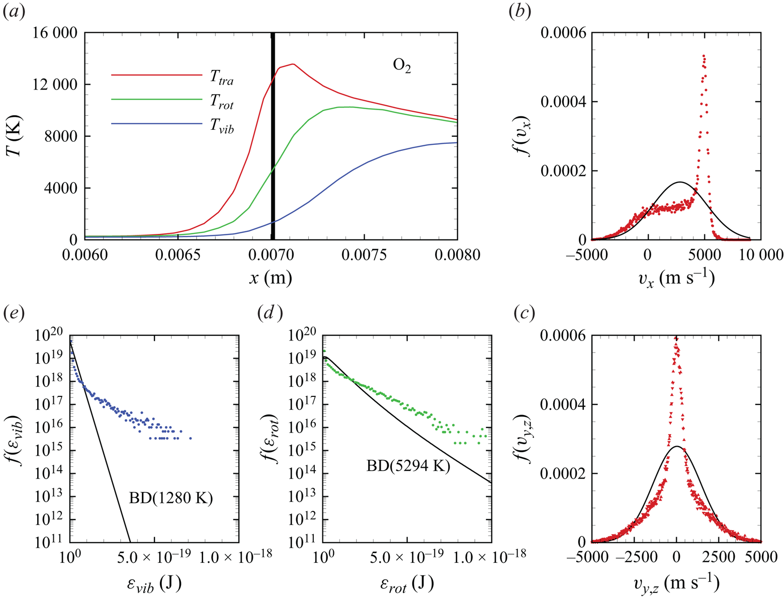
Figure 18. Molecular oxygen velocity and internal energy distributions extracted along the stagnation line shown in (a) at the location marked by the grey vertical line; (b–c) velocity distributions, (d) rotational energy distribution and (e) vibrational energy distribution.
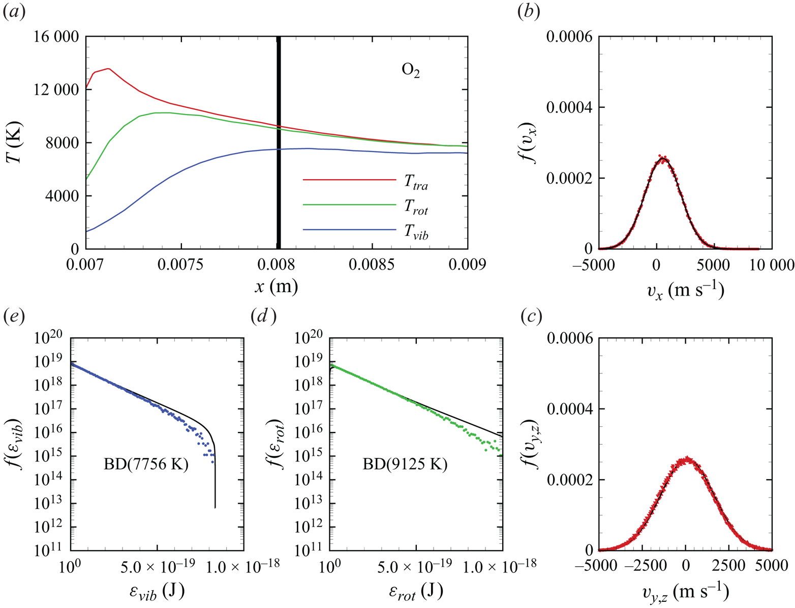
Figure 19. Molecular oxygen velocity and internal energy distributions extracted along the stagnation line shown in (a) at the location marked by the grey vertical line; (b–c) velocity distributions, (d) rotational energy distribution and (e) vibrational energy distribution.
The significant thermal non-equilibrium that characterizes strong shock waves is particularly well highlighted by the velocity distributions for each translational velocity component, shown in figure 18(b). Since the flow direction is along  $x$,
$x$,  $f(v_x)$ shows a well-known bimodal shape (Valentini & Schwartzentruber Reference Valentini and Schwartzentruber2009; Torres & Schwartzentruber Reference Torres and Schwartzentruber2022) that is indicative of a mixture of high-speed, low-temperature, pre-shock particles and low-speed, high-temperature, post-shock particles. The distributions for
  $v_y$ and
  $v_z$, shown in figure 18(c), exhibit a narrower structure compared with the corresponding equilibrium Maxwell–Boltzmann function obtained at the same average translational energy. This is too the result of the mixing of pre-shock and post-shock molecules.
Rotational and vibrational energy distributions are shown in figures 18(d)–18(e), where the distinct overpopulation of the high-energy tails is evident. The strong thermal non-equilibrium at this location is determined by the time lag of internal energy relaxation with respect to translational modes, which is more significant for vibration (VT energy transfer) than rotation (rotation–translation energy transfer), as shown by the rotational populations being closer to the corresponding equilibrium Boltzmann distribution than the vibrational energy populations. In this collisionally hot environment ( $T_{tra} \simeq 12\,000$ K), excitation of internal energy modes is manifested by the relative increase of
  ${\rm O}_2$ molecules occupying high-energy states, as also previously observed in other DMS computations (Valentini et al. Reference Valentini, Grover, Bisek and Verhoff2021; Torres & Schwartzentruber Reference Torres and Schwartzentruber2022; Grover et al. Reference Grover, Verhoff, Valentini and Bisek2023b).
The same molecular-level distributions for  ${\rm O}_2$ were obtained at another, further downstream, location along the stagnation line, shown in figures 19(a)–19(e). A total of nearly one million oxygen molecules were collected at
  $x=0.008$ m, using the same protocol described before and in a region
  $x\in [0.00800,0.00802]$ m and
  $y\in [0,0.0005]$ m. At variance with the earlier location, translational modes are in thermal equilibrium, as indicated by their Maxwell–Boltzmann velocity distributions shown in figures 19(b)–19(c). As discussed in § 5.1, molecular oxygen is rapidly dissociated in the hot shock layer produced at the conditions of this flow. The coupling between fast dissociation and slow vibrational excitation results in a QSS temperature profile along the stagnation line. As widely discussed in previous works (Valentini et al. Reference Valentini, Schwartzentruber, Bender, Nompelis and Candler2015; Grover et al. Reference Grover, Torres and Schwartzentruber2019b; Torres & Schwartzentruber Reference Torres and Schwartzentruber2020), QSS is characterized by distributions that have depleted high-energy tails. This is evident in both the rotational and the vibrational probability densities that are shown in 19(d)–19(e).
Qualitatively similar distributions to those of molecular oxygen were obtained for  ${\rm N}_2$, as shown in figures 20(a)–20(e). Approximately 4 million nitrogen molecules were collected at
  $x=0.00888$ m, in a region
  $x\in [0.00888,0.00890]$ m and
  $y\in [0,0.0005]$ m. Molecular nitrogen translational modes are in equilibrium, as shown by the Maxwell–Boltzmann velocity distributions shown in figures 20(b)–20(c). At variance with molecular oxygen, however, molecular nitrogen dissociation is minimal. At these conditions, the impact of vibrational energy removal on the internal energy distributions is not significant. Therefore, the rotational and the vibrational energy probability densities, shown in 20(d)–20(e), follow equilibrium distributions at the corresponding macroscopic temperature (nearly 7800 K).
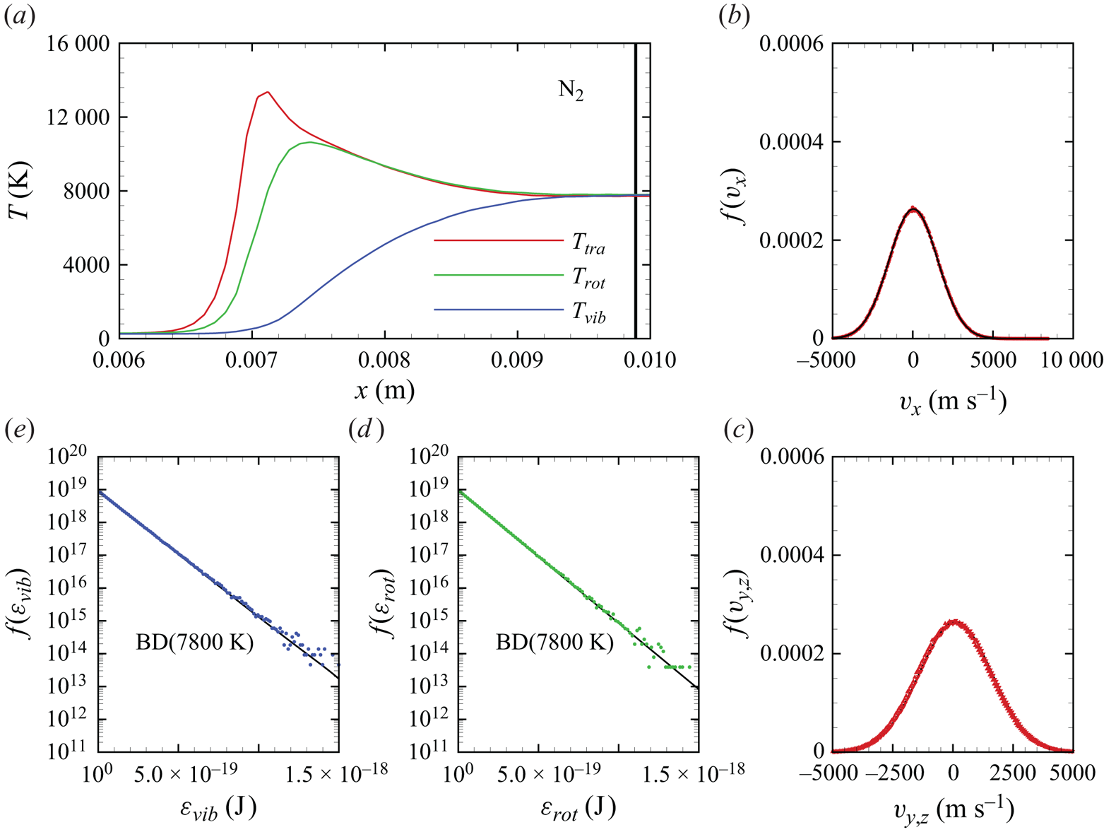
Figure 20. Molecular nitrogen velocity and internal energy distributions extracted along the stagnation line shown in (a) at the location marked by the grey vertical line; (b–c) velocity distributions, (d) rotational energy distribution and (e) vibrational energy distribution.
Distributions for internal energies and translational velocities were sampled for NO at two locations along the stagnation line, namely for  $x\in [0.00888,0.00890]$ m and for
  $x\in [0.00988,0.00990]$ m. A total of nearly 1.7 million and 1 million NO molecules were collected at each location, respectively. Notably, the first location roughly corresponds to the peak of NO concentration, whereas the second location is very close to the stagnation point, where some NO has been consumed by either dissociation or exchange processes. Molecular translational velocities are distributed according to the equilibrium Maxwell–Boltzmann distribution, as illustrated in figures 21(b)–21(c) and 22(b)–22(c). Furthermore, as shown in figures 21(c)–21(d) and 22(c)–22(d), internal energy distributions for rotational and vibrational energy appear to be at near equilibrium. This is somewhat at variance with the study of Torres et al. (Reference Torres, Geistfeld and Schwartzentruber2024), where vibrational energy distributions were shown to exhibit a depletion of high-energy states due to the dissociation process in a chemical reactor thermostatted at 8000 K. A potential explanation for this difference could be attributed to the presence of
  ${\rm N}_2+{\rm NO}$ collisions, which were not included by Torres et al. (Reference Torres, Geistfeld and Schwartzentruber2024). These collisions, which are here described by a semi-empirical surface, could be responsible for a faster replenishment of such high-energy states, thus diminishing the net effect of vibrational energy removal from the QSS distributions. An alternative explanation could be due to insufficient statistics gathered here to resolve the very high-energy tail of the distributions, as molecules have to be extracted in a near-pointwise fashion, therefore limiting the total available number of particles used to obtain these statistics. Finally, we point out that particles were extracted along a finite, albeit small,
  $y$ length (
 $y\in [0,0.001]$ m), thus producing a smearing of the samples over the gradients along the
  $y$ axis.

Figure 21. Nitric oxide velocity and internal energy distributions extracted along the stagnation line shown in (a) at the location marked by the grey vertical line; (b–c) velocity distributions, (d) rotational energy distribution and (e) vibrational energy distribution.
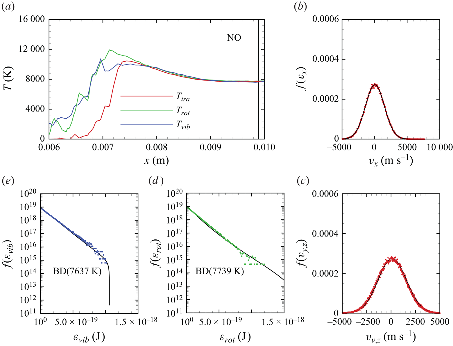
Figure 22. Nitric oxide velocity and internal energy distributions extracted along the stagnation line shown in (a) at the location marked by the grey vertical line; (b–c) velocity distributions, (d) rotational energy distribution and (e) vibrational energy distribution.
5.3. Mass diffusion phenomena
In a multi-component gaseous mixture, particularly when subjected to strong local variations of temperature, composition and pressure, the diffusion velocity of each chemical species is a complex function of the various thermochemical gradients (Hirshfelder, Curtiss & Bird Reference Hirshfelder, Curtiss and Bird1964). The diffusion velocity  $\boldsymbol {v}_{d}^{i}$ is defined as the rate of flow of a given species
  $i$ in a reference frame moving with the local average velocity of the mixture
 \begin{equation} \boldsymbol{v}_{d}^{i} = \boldsymbol{V}^{i} - \boldsymbol{u}, \end{equation}
where  $\boldsymbol {V}^{i}$ and
  $\boldsymbol {u}$ are the species and mixture velocities, respectively, in the laboratory reference frame. The mass flux vector
  $\boldsymbol {j}^{i}$ is then
 \begin{equation} \boldsymbol{j}^{i} = \rho^{i} \boldsymbol{v}_{d}^{i}. \end{equation}
 In figure 23, we plot the projection of  $\boldsymbol {j}^{i}$ onto the local flow velocity unit vector
  $\boldsymbol {\hat {u}}=\boldsymbol {u}/|\boldsymbol {u}|$, rescaled with the local total mass density
 \begin{equation} \upsilon^{i} = \boldsymbol{v}_d^{i} \boldsymbol{\cdot} \boldsymbol{\hat{u}}. \end{equation}
The quantity  $\upsilon ^{i} \rho ^i/\rho$ represents the diffusion velocity of species
  $i$ with respect to the local flow velocity along a streamline in the flow. A negative
  $\upsilon ^{i}$ indicates that molecules of species
  $i$ are lagging with respect to other species present in the mixture.
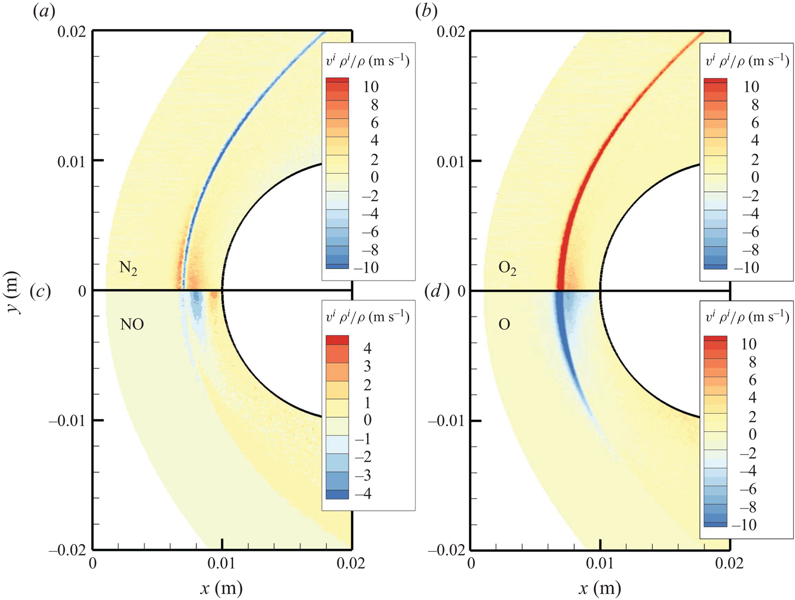
Figure 23. Density-scaled mass diffusion flux for (a)  ${\rm N}_2$, (b)
  ${\rm O}_2$, (c) NO and (d) O across the flow field.
In figure 23, we plot  $\upsilon ^{i} \rho ^i/\rho$ for the most abundant species in the flow. As shown in figures 23(a)–23(b), molecular nitrogen and molecular oxygen show an opposite behaviour at the shock front, where strong gradients of temperature and pressure are present. In particular, molecular nitrogen is shown to lag molecular oxygen. This can be attributed to the mass differential between the two species, with the heavier one fluxing through the shock front at a faster rate (Valentini et al. Reference Valentini, Tump, Zhang and Schwartzentruber2013). Qualitatively similar behaviour to
  ${\rm N}_2$ is displayed by atomic oxygen, shown in figure 23(c) due to its smaller mass compared with its molecular counterpart. The variation of
  $\upsilon ^{i} \rho ^i/\rho$ for NO, however, is much more complex and displays positive and negative values, particularly along the stagnation line. This behaviour is potentially the result of the coupling between thermal and barometric gradients with the chemical activity responsible for NO production and removal near the stagnation point. This complexity is better highlighted by the trends for
  $\upsilon ^{i} \rho ^i/\rho$ along the stagnation line that are shown in figure 24. These results provide a stringent test case for more refined descriptions for the mass flux vector where the contribution of temperature and pressure gradients could be also included.

Figure 24. Density-scaled mass diffusion flux for  ${\rm N}_2$,
  ${\rm O}_2$, NO, N and O along the stagnation streamline.
Finally, all the potentials used in our work were constructed with a focus on high-energy collisions, characteristic of the hot shock layer. Hence, long-range forces are less accurate, as discussed by Garcia, Martínez & Laganà (Reference Garcia, Martínez and Laganà2015) for instance. In the flow presented here, however, temperatures in the shock layer reach approximately 8000 K. Therefore, it is not expected that dispersion terms have a significant influence on transport properties. For other flows, particularly those dominated by strong expansions (e.g. nozzle flows), an improved description of long-range attractive forces between particles may become necessary.
6. Conclusions
In this work, we have simulated a Mach 15 air flow over a blunt wedge using the DMS method. The resulting air mixture around the wedge only contains  ${\rm N}_2$,
  ${\rm O}_2$, NO, N and O in their ground electronic states. This system is typically referred to as five-species air. To isolate gas-phase chemistry from gas–wall viscous interactions, we modelled the wedge wall as an inviscid surface. Therefore, no velocity or temperature boundary layers form. Future work will address viscous wall effects as well.
All PESs that were used to model the various air molecules interactions were obtained from first principles using the quantum mechanics dictated statistical weights. Two exceptions, namely  ${\rm N}_2+{\rm NO}$ and
  ${\rm O}_2+{\rm NO}$, had to be made. To our knowledge, these PESs are not available in the literature and have not been validated for their applicability to high-temperature gas phenomena. Therefore, semi-empirical surrogates were used for these interactions to guarantee that all collisions responsible for mass, momentum and energy transfer in the flow were accounted for. To further increase the realism of air simulation, however, it is hoped that ab initio PESs for
  ${\rm N}_2+{\rm NO}$ and
  ${\rm O}_2+{\rm NO}$ interactions will be produced in the future.
For the given free-stream conditions, significant vibrational non-equilibrium was observed in the shock layer. Rotational non-equilibrium was only confined to the shock structure, and  ${\rm N}_2$,
  ${\rm O}_2$ and NO rotational energy modes were equilibrated with the translational modes in the majority of the shock layer. The flow exhibited significant chemical reactivity, with near-complete oxygen dissociation and conspicuous formation of NO. Molecular nitrogen dissociation was of secondary importance, as the temperatures reached in the shock layer hardly exceeded 8000 K. Complex mass diffusion kinetics were identified in the shock layer by an analysis of each species diffusion velocity. This was particularly pronounced at the bow shock interface, due to its strong gradients of temperature and pressure. It was also observed that the lighter species were lagging behind the heavier molecules.
The use of DMS not only provides a complete understanding of the macroscopic system, it can also provide microscopic-level details of the flow. In practice, statistics for external and internal energy modes can be gathered at various locations throughout the flow. Here, we extracted several velocity and energy distributions for  ${\rm N}_2$,
  ${\rm O}_2$, and NO along the stagnation streamline, given its importance. The chemical kinetics that characterize this flow cause rotational energy and vibrational energy distributions for
  ${\rm N}_2$ and
  ${\rm O}_2$ to exhibit the familiar features consistent with the strong coupling between energy removal due to dissociation and vibrational excitation. Nitric oxide, a species that is produced in the shock layer due to the reaction between O and
  ${\rm N}_2$, exhibits a peculiar trend. Namely, it was formed vibrationally hot. Further, its temperature equilibration was quite rapid. We attribute this behaviour to the nature of its formation via exchange processes that result in products that have no memory of any initial state. However, we cannot exclude that the fast equilibration was also the result of the semi-empirical PES that describes
  ${\rm N}_2+{\rm NO}$ interactions. This process should, therefore, be revisited when these ab initio PESs become available. Translational modes of the atoms (N and O) are shown to quickly equilibrate with those of the molecules. As no electronically excited states are present, translational velocities distributions are sufficient to characterize the state of atomic particles and they were shown to align well with the equilibrium Maxwell–Boltzmann probability density.
All these physical phenomena directly couple to the mechanics of the gas flow and are all solely traceable to the PES inputs, without the need for any other thermochemical models or assumptions, or a constitutive or mixing law for transport properties. As such, this DMS solution is obtained from a self-contained framework for all the coupled gas physical phenomena. At the imposed conditions, this flow remains in the near-continuum regime and, therefore, it provides a stringent test case for enhancing the fidelity of thermochemical and transport models used in CFD codes for hypersonic flow simulation.
Acknowledgements
The authors gratefully acknowledge funding from the Air Force Office of Scientific Research (AFOSR) through contract LRIR 24RQCOR009. Use of computational resources made available through the Department of Defense High Performance Computing Modernization Program (HPCMP) is greatly appreciated. We would also like to thank Dr D. Andrienko at the University of Colorado for kindly providing us with the semi-empirical surfaces for  ${\rm N}_2+{\rm NO}$ and
  ${\rm O}_2+{\rm NO}$ interactions.
Funding
LRIR 21RQCOR045.
Declaration of interests
The authors report no conflict of interest.
Data availability statement
The data that support the findings of this study are available from the authors upon reasonable request.
Author contributions
The authors confirm contribution to the paper as follows: P.V.: conceptualization, data curation, formal analysis, investigation, methodology, validation, writing – original draft preparation and writing – review and editing; M.S.G.: conceptualization, writing – review and editing; and N.J.B.: project administration, funding acquisition and writing – review and editing.
Appendix A. Removal of semi-empirical  ${\rm N}_2+{\rm NO}$ and ${\rm O}_2+{\rm NO}$ surfaces


To highlight the problem related to the absence of collisions of NO with either  ${\rm N}_2$ or
  ${\rm O}_2$, we restarted the steady-state solution but switched off the interactions described by the semi-empirical
  ${\rm N}_2+{\rm NO}$ and
  ${\rm O}_2+{\rm NO}$ surfaces.
The resulting evolution of the system is shown in figures 25(a)–25(b). As NO particles now undergo no collisions with  ${\rm N}_2$, i.e. the most abundant species in the flow, they diffuse upstream forming a quasi-collisionless expanding flow. This is evidenced by
  $T_{tra}< T_{rot}$ and
  $T_{tra}< T_{vib}$. Moreover, the NO concentration increases upstream of the shock wave, while decreasing near the stagnation region.
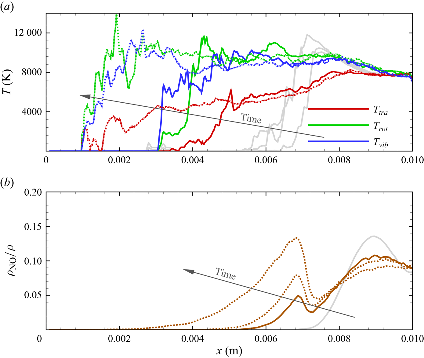
Figure 25. Time evolution of the NO temperature profiles and mass fraction along the stagnation line when  ${\rm N}_2+{\rm NO}$ and
  ${\rm O}_2+{\rm NO}$ interactions are ignored.
Appendix B. Molecular trajectory dynamics
Trajectories are time integrated using the MD technique. The Newtonian dynamics for the interacting pair (molecule–molecule, molecule–atom or atom–atom) is solved by integrating the equation of motions on one of the prescribed PESs listed in table 1. The set of ordinary differential equations for Newtonian motion is then numerically propagated in time
 $$\begin{gather} \dot{\boldsymbol{r} }_i = \boldsymbol{v}_i, \end{gather}$$
 $$\begin{gather}\boldsymbol{F}_i ={-}\sum_{j=1}^N \frac{\partial \psi(r_{ij})}{\partial r_{ij}}\frac{\boldsymbol{r}_{ij}}{r_{ij}}, \end{gather}$$
where  $\boldsymbol {r}_i$ and
  $\boldsymbol {v}_i$ are the position and velocity vectors of atom
  $i$, respectively. The potential function (PES) is
  $\psi (r_{ij})$, generally a function of 6 (
 $N=4$, e.g.
  ${\rm O}_2+{\rm O}_2$), 3 (
 $N=3$, e.g.
  ${\rm O}_2+{\rm O}$) or 2 (
 $N=2$, e.g.
  ${\rm O}+{\rm O}$) interatomic distances
  $r_{ij}$. Since no electronic excitation is considered in this work,
  $\psi$ represents the adiabatic electronic-ground-state PES.