At the core of modern political economy theory is the idea that income drives political preferences. Since Downs’Footnote 1 seminal contribution, the workhorse models of redistributive politics characterize individuals by income to generate key predictions;Footnote 2 other factors such as ideology or multi-dimensional preferences are then introduced to complicate this basic framework.Footnote 3 Indeed, the starting point for micro-founded models of all manner of political economy phenomena—including growth, redistribution and transitions to democracy—is to write a utility function in which agents are differentiated by income. Other literatures, such as class-based interpretations of citizen activism and welfare state expansion, also explicitly or implicitly assume that income plays a key role in driving political behavior.Footnote 4
Surprisingly, despite its centrality to foundational research agendas in economics, political science and sociology, we lack clear evidence of income’s effect on political preferences. Empirical findings range widely; some studies report that income strongly predicts conservative political preferences, while others find small (or even negative) effects. In the American context, several analyses report relatively small differences between the poor and wealthy with respect to public policy preferences and political party support.Footnote 5 Other studies find substantial and increasingly strong income effects, arguing that income predicts Republican partisanship and presidential voting since the 1950s,Footnote 6 and that support for increased spending on redistributive and welfare state policies declines markedly with income.Footnote 7
Outside the United States, the evidence is similarly mixed. Single-country studies often find that voters’ evaluations of their own personal economic situations are a relatively unimportant determinant of vote choice; cross-country analyses also report weak or even negative effects of income on propensity to vote for the right.Footnote 8 In Norris’Footnote 9 analysis of the sources of voting behavior in thirty-seven countries, for example, income influences voting in the predicted direction (lower-income individuals supporting left parties) in only one-third of the sample. De La O and RoddenFootnote 10 conclude that the empirical basis for formal political economy models is weak in that income poorly predicts voting behavior and that any effect is driven by the top income quartile. And yet, several other comparative studies of voting behavior and the rich–poor voting gap suggest that wealthier voters tend to exhibit more conservative preferences and voting patterns.Footnote 11
One factor that may be driving these different estimates is measurement error of income. In cross-sectional analysis, classical measurement error will attenuate estimates toward zero. More problematic is the possibility that the rich may disproportionately under-report income on a survey, yielding underestimates of income’s effect on political behavior. Income fluctuations offer another potential explanation for the mixed findings in the literature. If political preferences are driven by permanent income, as predicted by many political economy models, we will tend to underestimate the causal relationship due to the volatility reflected in annual measures of income.
More broadly, the wide disparity of estimates suggests that income’s effect on political preferences is highly subject to sensitivity to model specification. This is most clearly seen in studies that report divergent results even when using the same data. Using the same British data analyzed in this article, Brynin and Sanders and Sanders and Brynin find small and statistically insignificant effects of income on voting, while Oswald and Powdthavee report that high-income people lean rightward.Footnote 12 This suggests that merely adding additional control variables to regression models will not alleviate problems of inference.
Spurred by such disparate findings, this article draws from the toolkit of anthropologists and economists to offer a novel measure to capture the effect of economic well-being on political behavior: height. Scholars outside of political science have long used height to assess affluence among historical populations in the absence of detailed information on income and wealth. Modern social surveys that collect both anthropometric measures and information on income have confirmed the relevance of height as a proxy for income. A wide range of studies has documented a robust relationship between height and income at both the aggregate and individual levels across multiple settings. At the national level, Steckel finds that average height moves with a country’s level of economic development.Footnote 13 Numerous micro-level studies also find a sizeable height premium in the labor market. For example, Case and Paxson find that for both men and women, an additional inch of height is associated with a 1–2 per cent increase in earnings.Footnote 14 Similarly, Persico, Postlewaite and Silverman find that among white males in Britain and the United States, the tallest quarter of the population has a median wage that is more than 13 per cent higher than that of the shortest quarter.Footnote 15 Thus, although scholars debate the precise channels through which height affects income,Footnote 16 the general finding of a direct relationship remains robust. For these reasons, Mankiw and Weinzierl argue (albeit somewhat tongue in cheek), that taller individuals should be taxed on utilitarian grounds, and produce example tax tables calibrated to the height–earnings premium.Footnote 17
If our goal is to capture a more general sense of economic well-being, height arguably enjoys many advantages relative to income. First, height is increasingly collected in modern surveys, and self-reported height is arguably less prone to measurement error than income. Moreover, it is substantially easier to verify a respondent’s height in the course of administering a survey. Finally, unlike income, height is not subject to annual fluctuations. It thus proxies for permanent income, which drives preferences in canonical political economy models.Footnote 18
By focusing on the relationship between economic well-being and political preferences, our article complements—but is distinct from—two related strands of the literature on economic voting. First, we are not principally concerned with the dynamic interplay between income fluctuations and voting behavior—what is typically termed pocketbook voting. Secondly, we do not focus on the extent to which individuals punish or reward incumbents based on macroeconomic conditions. Instead, our use of height aims to generate a measure of permanent economic well-being, motivated by the core models of political economy, which posit income as central to the choice of tax rate and the optimal size of government.
DATA
In order to explore the relationship between height and political outcome measures we use data from 2006 (Wave 16) of the British Household Panel Study (BHPS), a nationally representative sample of the adult population in Britain.Footnote 19 The BHPS contains data from approximately 5,000 households and over 12,000 adults, interviewed from 1991 onward in the autumn of each year. This dataset has clear attractions for our purposes. First, it contains self-reported height data as well as detailed income data. Equally important, the BHPS provides a number of political variables, such as party support, policy preferences and vote choice. Finally, the BHPS offers a rich set of control variables, including educational attainment, religious affiliation and ethnicity.
Our central dependent variable is a binary Supports Conservatives, coded as 1 if the respondent supports the Conservative Party, and 0 otherwise. We focus foremost on party support, which we believe offers the most stringent test of the core claims of political economy models, since individuals often announce a greater desire for redistribution than is revealed in the actual support for a party that would likely redistribute income away from them.Footnote 20 Another useful feature of the BHPS is that it contains multiple questions on policy preferences, enabling the investigation of various dimensions of political behavior. We consider a series of policy preferences that probe specific aspects of government intervention in markets. Finally, we examine actual political behavior: voting conditional on turnout.
To operationalize the dependent variable, we use the ‘Economic Dimension’ (dimension 1) from Benoit and Laver’s Party Policy in Modern Democracies (PPMD) project to order British parties according to their support for redistribution.Footnote 21 As Huber and StanigFootnote 22 note, this measure is useful for positioning parties on the dimension most relevant for testing workhorse political economy models: the tax-and-transfer scale. In the PPMD data, country experts place parties on a scale from 1 (‘promotes raising taxes to increase public services’) to 20 (‘promotes cutting public services to cut taxes’). The data support our ordering of the British political landscape into Conservative versus non-Conservative: the Conservative Party receives a score of 15.3, far right of Labour’s 8.1 and the Liberal Democrats’ 5.8; the average of all UK parties is 6.3, with a standard deviation of 1.3. This expert-based ranking, with the Conservatives furthest to the right, is well in line with positioning based on party manifestos.Footnote 23
Height is measured in inches; both height and income are winsorized at 0.5 per cent to deal with implausibly extreme values. Our sample consists of respondents aged eighteen and above living in England, Scotland and Wales. We exclude Northern Ireland from the estimation sample due to their very different political environment, although we report all-inclusive specifications in our robustness checks. Summary statistics, presented in the Appendix, indicate that our variables of interest look reasonable. For both men and women, height is normally distributed, with men on average being six inches taller than women. Approximately 25 per cent of the sample supports the Conservative Party; this is the case for both men and women.
HEIGHT AND POLITICAL PREFERENCES
The first key result of this article is that taller people are more likely to support the Conservative Party and to hold conservative political positions. This pattern can be seen in Figure 1, which plots the propensity to support the Conservative Party on height, using a multivariate smoother to control for age and gender. We see that support for the Conservatives moves steadily with height across the bulk of the distribution; for this group, the relationship is almost linear, moving from a predicted value of around 0.2 at the 10th percentile of height to 0.3 at the 90th. Interestingly, support for the Conservatives flattens (and even dips slightly) at the top of the height distribution. This drop in Conservative support among extremely tall individuals is consistent with a dip in income among this group, which we discuss below.Footnote 24
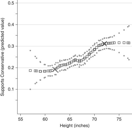
Fig. 1 Taller people support Conservatives Note: Running line smooth of ‘supports Conservative party’ on height, adjusted for age and gender. The Xs mark the 10th and 90th percentile of the height distribution; 95 per cent pointwise bootstrapped confidence intervals displayed.
We next investigate the effect of height parametrically. Formally, we estimate linear probability models of the form:
where V is our political variable, H is height, and X is a matrix of covariates. All specifications here and throughout the article report heteroskedasticity-robust standard errors, clustered by household, which allows for common household shocks correlated across individuals.
The coefficient of interest, ϕ, is the direct effect of height on support for the Conservatives. In the second row of Table 1, we estimate this effect. Here and throughout, we suppress the complete regression output; full tables for all results are reported in the Appendix. Column 1 employs an extremely simple specification, including as controls only age, sex and region. Here, we find that each additional inch yields a 0.8 percentage point higher probability of supporting the Conservative Party. In Column 2, we add controls for race, years of schooling, marital status and religion. These slightly reduce height’s effect to 0.6 percentage point per inch, translating to a one standard deviation increase in height yielding a 2.4–3.2 percentage point higher probability of supporting the Conservatives. In sum, the regression results of the direct relationship between height and Conservative support reinforce the pattern seen in the raw data.
Table 1 Political Effects of Height

Note: least squares regression of ‘supports Conservative Party’ on height. Extended controls include: married, white, years of schooling, religion. Full models reported in the Appendix. Heteroskedasticity-robust standard errors, clustered by household. Statistical significance: *10%; **5%; ***1%.
This result is robust to changes in the estimation sample and alternative functional forms. In Columns 3 and 4 of Table 1, we consider an age-restricted sample. Since we want our height variable to proxy for long-term physical well-being, we estimate specifications including only prime-age individuals (eighteen to sixty-five). This approach avoids inadvertently capturing health factors that slow youths’ attainment of their adult heightFootnote 25 or increase shrinkage of the elderlyFootnote 26 —such factors could potentially contaminate our research design by acting as a direct impetus for favoring robust national health care. In results reported in the Appendix, we show that the findings are robust to including residents of Northern Ireland in the sample and to the use of height as collected in Wave 14. In the Appendix we also reproduce all linear probability estimates using logit and probit, and ordered-response models using ordered logits and ordered probits. For all results, average marginal coefficients are qualitatively similar.
The relationship between height and political preferences identified here is not an artifact of relying on a single outcome, but instead is consistent across an array of political preferences and behavior. Although the BHPS does not directly probe individuals’ preferred levels of taxes and transfers, it does ask a series of questions about the relative balance that should be struck between the state versus the market. Respondents are asked the extent to which they support (a five-point ordinal measure, from −2 ‘strongly disagree’ to 2 ‘strongly agree’) the following statements: ‘Private enterprise is the best way to solve the UK’s economic problems’; ‘Major public services and industries ought to be in state ownership’; ‘The government should place an upper limit on the amount of money that any one person can make’; and ‘It is the government’s responsibility to provide a job for everyone who wants one’. Finally, given that stated values and voting behavior can differ dramatically,Footnote 27 we also explore the relationship between height and conservative voting.
The association between height and these preferences is presented in Figure 2. All are broadly consistent with the results from ‘support Conservative’: taller people look more favorably on private enterprise and less favorably on the need for state ownership of public services, government provision of jobs and state-mandated limits on earnings. As with Conservative support, the estimated effect is close to linear over the bulk of the distribution, and flips at the top of the height distribution. The same pattern holds when we parametrically examine height’s effect, in Columns 1–4 of Table 2. Here, we treat each dependent variable as continuousFootnote 28 and estimate Equation 1, including controls for age, sex, race, religion, years of schooling, marital status and region. Consistent with the figure, point estimates are larger for government provision of jobs and state-mandated limits on earnings.Footnote 29 Finally, Figure 3 shows that the positive relationship between height and Conservative voting conditional on turnout also holds. Including controls in a regression framework, Column 5 of Table 2 shows that each additional inch is associated with a 0.5 percentage point increase in the propensity to vote for the Conservative Party.
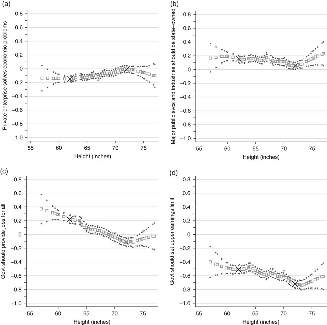
Fig. 2 Height’s political consequences: policy preferences Note: Running line smooth of (a) ‘Private enterprise is the best way to solve the UK’s economic problems’; (b) ‘Major public services and industries ought to be in state ownership’; (c) ‘It is the government’s responsibility to provide a job for everyone who wants one’; and (d) ‘The government should place an upper limit on the amount of money that any one person can make’ on height, adjusted for age and gender. Each dependent variable indicates strength of support, ranging from −2 (strongly disagree) to 2 (strongly agree). The Xs mark the 10th and 90th percentile of the height distribution; 95 percent pointwise bootstrapped confidence intervals displayed.
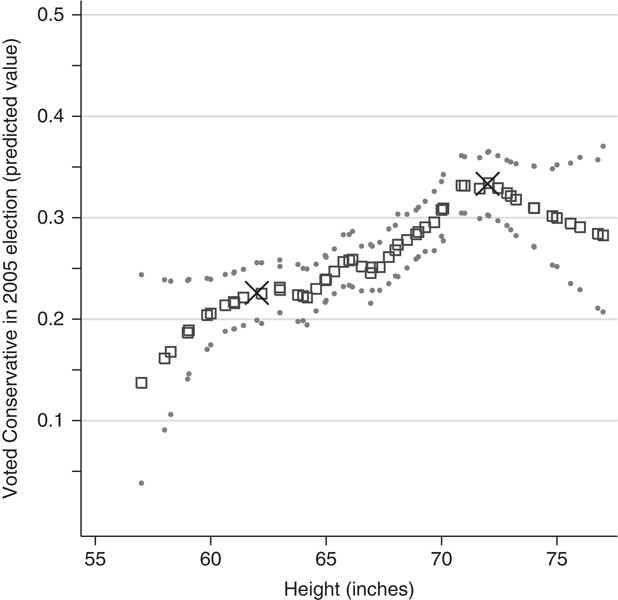
Fig. 3 Taller people vote for Conservatives Note: Running line smooth of ‘Voted for Conservative Party in 2005 general election’ on height, adjusted for age and gender. The Xs mark the 10th and 90th percentile of the height distribution; 95 per cent pointwise bootstrapped confidence intervals displayed.
Table 2 Height and Policy Preferences

Note: direct relationship between height and political preferences. Dependent variables are (1) ‘Private enterprise is the best way to solve the UK’s economic problems’; (2) ‘Major public services and industries ought to be in state ownership’; (3) ‘It is the government’s responsibility to provide a job for everyone who wants one’; (4) ‘The government should place an upper limit on the amount of money that any one person can make’; and (5) ‘Voted for Conservative Party in 2005 General Election’. Each dependent variable indicates strength of support, ranging from −2 (strongly disagree) to 2 (strongly agree). Extended controls include: married, white, years of schooling, religion. Full models reported in the Appendix. Heteroskedasticity-robust standard errors, clustered by household. Statistical significance: *10%; **5%; ***1%.
Alternative Channels
One concern in employing height as a proxy for economic well-being is that it may be picking up other factors that drive political behavior. For instance, Case and PaxsonFootnote 30 argue that the early life circumstances that determine adult height also generate cognitive advantages. If these cognitive advantages directly affect political preferences, this will contaminate the interpretation of the height effect. This problem is probably less relevant in our setting precisely because existing research offers mixed evidence that cognition directly affects partisan support. Studies based on US data suggest that it has a negligibleFootnote 31 or inconsistentFootnote 32 effect on political preferences. In contrast, a study from BritainFootnote 33 finds that cognition is associated with left voting, while two Swedish studies suggest the opposite: that it increases support for right-wing policies and reduces support for redistribution.Footnote 34 If we consider education as a proxy for cognition, cross-country work is more consistent, finding that schooling acts as a cross-cutting cleavage with respect to income: although income may induce individuals to vote conservative, those with more education are more likely to hold left-wing political values and to vote for left-wing parties,Footnote 35 especially in wealthy nations such as Britain.Footnote 36
Given the clear lack of consensus in the literature, we generate a control for cognition. While our data do not permit a direct measure of cognitive ability, we take two steps to assess cognition’s potential as a channel through which height shapes political preferences. First, we add education in the form of years of schooling to the regression model. While years of schooling is probably a poor proxy for innate cognitive ability, we find that height’s effect on Conservative support is demonstrated in specifications with and without this measure. Secondly, in the British setting, studies of cognition have found that cognitive ability test scores correlate well with scores on O-level and GCSE examinations;Footnote 37 fortunately, information about these examinations is available in the BHPS. We follow Deary et al.Footnote 38 intelligence in constructing a measure that assigns point values to each high versus low O-level/GCSE pass received by an individual. Column 5 of Table 1 shows that the point estimate on height remains positive and strongly significant even when we include this proxy measure for cognitive ability as a control. The result is robust to using alternative measures, such as the number of GCSE passes, restricting only to high passes, and other variations on this theme.
Another possible channel through which height may drive Conservative support is through parents’ background. For example, if parents’ income and political orientations during childhood predict height, then these parental influences may directly shape one’s political preferences, rendering height a proxy for parents’ characteristics rather than economic well-being. We test this potential explanation directly using the BHPS youth survey. For this sample of children (aged eleven to seventeen) of main survey respondents, we can link children’s height to various self-reported parental characteristics of interest: income, years of schooling and Conservative support.Footnote 39 Table 3 illustrates that these parental characteristics have very little predictive power over children’s height. The coefficients for father’s and mother’s support for the Conservatives are negative, although substantively small and statistically insignificant—this is also the case for father’s schooling. The coefficients on mother’s schooling and parents’ income, although slightly positive, are also small and statistically insignificant.
Table 3 Child Height and Parents’ Characteristics
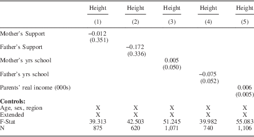
Note: least squares regression; dependent variable is height (in inches) for youths aged eleven to seventeen. Each row represents a separate regression. All specifications include age, sex, race, religion and region controls. Full models reported in the Appendix.
This finding militates against height serving as a proxy for parental political preferences. As an alternative strategy of assessing the influence of parents’ characteristics, we employ models that explicitly control for family background characteristics: father’s and mother’s highest educational attainment, and father’s score on the Hope Goldthorpe scale (HGS). The HGS, commonly used in British analyses of social class, is an occupational index that classifies jobs according to their social desirability. The scale is an updated version of a 1974 survey of the social standing of various occupations in Britain. Occupational groups in the BHPS are collapsed into thirty-six categories and then ranked according to their reputation. The final ordering assigns scores between 0 (unavailable occupation or employment status) and 82 (occupation with the highest reputation). While in principle the score is a useful measure of social background, the HGS is often difficult to recover from retrospective data. In our case, including the score cuts the sample size by 25 per cent, and missings are very likely nonrandom. Results are displayed in Columns 6 and 7 of Table 1. In Column 6, we add mother’s and father’s educational attainment to the most complete specifications from Table 1. Column 7 includes father’s HGS. In both cases, adding these family background variables to the model slightly decreases the point estimates, but overall the main finding of height’s strong and positive effects on support for the Conservatives holds. In fact, the decline in the point estimates is almost wholly due to the nonrandom nature of missing parental information. Reproducing the earlier Column 2 specification using only the respondents for whom parental characteristics are available yields almost identical coefficients to those in Columns 6 and 7.
The upshot, then, is that we have both direct and indirect reasons to doubt that cognition or parental characteristics are driving height’s effect on Conservative support.Footnote 40
OVER TIME AND GENDERED RESULTS
One attractive feature of our dataset is its longitudinal nature; while height was only elicited in Waves 14 and 16, we have information on income and political behavior dating back to the beginning of the panel.Footnote 41 Separately for each wave, we reproduce our specification with the extended set of controls corresponding to Column 2 of Table 1, and plot the results in Figure 4.
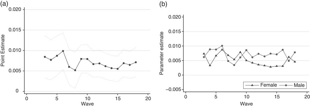
Fig. 4 Height and Conservative support over time Note: Point estimates and 95 per cent confidence intervals are produced in separate, wave-specific regressions, using the specification corresponding to Column 2 of Table 1. Panel (a) reports the direct effect of height on Conservative support; (b) reports these same models for men and women separately.
Starting with the direct relationship between height and political preferences reported in Panel (a), we see that the estimated effect of height on support for the Conservatives is broadly consistent over time. The estimated effect fluctuates a bit, spiking in Wave 6, falling in Waves 7 and 8, and then picking up to resume its original trajectory starting in Wave 9. However, the 95 per cent confidence intervals, while always excluding 0, are wide enough that we cannot reject a constant effect over time.
Given the rise of a political gender gap across advanced industrialized countries in recent years, another important question is whether the effects of income on political preferences vary substantially between men and women. To this point, all results have used the whole sample and controlled for gender; here, we split the sample by sex and reproduce our earlier specifications. For brevity, we choose two specifications to report in Columns 8–11 of Table 1: the simple specification (corresponding to Column 1 of Table 1), and the extended controls (corresponding to Column 2). These Wave 16 results suggest that the effect of height on political preferences is roughly twice as large for men than for women.
Panel (b) of Figure 4 explores whether these differences between men and women present in the Wave 16 data extend over time. In this figure, the plotted estimates reflect the effect of a one standard deviation increase in height (by wave and by gender) on Conservative support. We must be extremely cautious in interpreting this figure, as confidence intervals overlap over the entire period. This said, the broad pattern reflected in the estimates is striking. An additional inch of height increases the propensity of both men and women to support the Conservative Party, and for both sexes, height is associated with higher income. Although in both instances the estimated effects are usually higher for men than for women, given the size of the confidence intervals we cannot reject the null of no difference.
HEIGHT AS AN INSTRUMENT
Thus far, we have documented a robust positive relationship between height and political preferences, arguing that the most reasonable interpretation of this result is that economic well-being drives individual partisanship. In order to situate our findings, we pursue a thought experiment. Under the assumption that height’s effect on political preferences operates only through its effect on income, we can treat height as an instrumental variable that allows us to identify the effect of income on support for the Conservatives. This strategy enables us to make statements about the political effect of an additional thousand pounds of income, and to assess the extent of bias in existing ordinary least squares (OLS) estimates of income’s effects on political preferences.
Formally, we estimate two-stage least squares models of the following form, where V, H and X are as before, and I is income. Here, height is employed as an instrument to identify the first-stage equation:
The underlying logic of IV estimation is that the bias in OLS when a regressor is partially endogenous can be corrected by identifying another factor—the instrumental variable—that is correlated with the endogenous regressor and only affects the variable of interest through that channel, after controlling for other included regressors. More concretely, in our case, an instrumental variable should be sufficiently well correlated with income (relevant) and should only affect the outcome of interest insofar as it affects income (excludable: in Eq. 2, that
![]() ${\Bbb E}(h_{i} {\epsilon}_{i} )\,{\equals}\,0$
).
${\Bbb E}(h_{i} {\epsilon}_{i} )\,{\equals}\,0$
).
We argue that height is likely to meet both of these criteria. As to relevance, as we have seen, many studies find a strong relationship between height and income, and as we show below, height also strongly predicts income in the BHPS data. Indeed, F-statistics on the excluded instrument, reported at the bottom of Table 5, exceed conventional weak instruments thresholds. Excludability is a matter of judgement, and we believe that height is plausibly excludable for several reasons. First, as a measure of long-term physical well-being, height is unlikely to directly affect (or to be correlated with omitted variables that directly affect) political behavior other than through its ability to predict income. Unlike, for example, short-term health shocks or even chronic health conditions, height is unlikely to shape individuals’ preference for specific health policies (and hence their taste for redistribution). Instead, in our setting, height captures quasi-random shocks in early life that drive an individual to enjoy a higher income in adulthood, but are unlikely to directly affect the dependent variables of interest. For example, when we examined parental background in the previous section, we found little relationship between these characteristics and a child’s height, suggesting that height is indeed a credible source of exogenous variation.
In the IV models presented in Table 5, the central independent variable of interest is real annual income, measured in thousands of pounds. The income variable we use includes income from labor and non-labor sources, but does not include income from government transfers. Throughout we employ a standard set of control variables: age, sex, region, race, educational attainment and religion, the construction of which is detailed in the Appendix.
First Stage
To serve as an instrument variable, height must be a strong predictor of income. Figure 5 uses a multivariate smooth to plot income on height while controlling for age and gender. Income moves steadily with height, an almost linear relationship for the bulk of the distribution. Moving from the 10th to the 90th percentile of height is associated with an approximately £5,000 increase in income. At the very top of the height distribution, predicted income dips down, consistent with the pattern in Figure 1 of Conservative support.
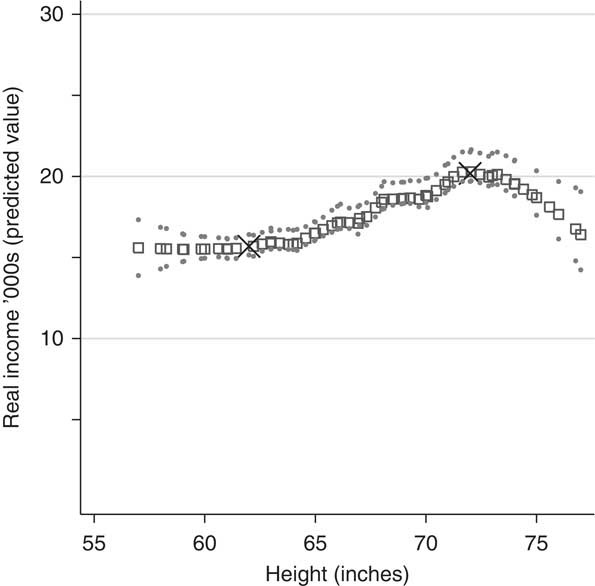
Fig. 5 Income and height Note: Running line smooth of ‘Real Income (’000s of pounds)’ on height, adjusted for age and gender. The Xs mark the 10th and 90th percentiles of the height distribution; 95 per cent pointwise bootstrapped confidence intervals displayed.
We estimate the first-stage relationship between income and height in Equation 2 in Table 4. The results shown in Columns 1 and 2, for example, show that height is a strong predictor of income; each additional inch translates into £200–350 of income, which in turn is 1–2 per cent of mean income—comparable to earlier waves of the BHPS.Footnote 42 These effects are highly statistically significant. Both from the raw data and from the regression results, the upshot is that height appears to be a good predictor of income and our estimated coefficients lie comfortably within the range identified in the literature.
Table 4 Instrumental Variables: First Stage
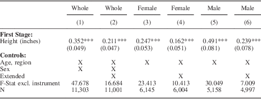
Note: dependent variable is ‘Real Income (’000s of pounds)’. First stage of 2SLS regression corresponding to Table 1. Extended controls include: married, white, years of schooling, religion. Full models reported in the Appendix. Heteroskedasticity-robust standard errors, clustered by household. Statistical significance: *10%; **5%; ***1%.
Should we be concerned about the self-reported nature of our height measure? In general, classical error in measurement of the instrumental variable will weaken the estimated effect of the instrument but will not bias the second-stage estimates of income’s effect on political preferences. As we have seen, the instrument is highly relevant, so this is not a concern in our data. This said, systematic misreporting of height, such that richer individuals disproportionately report being tall, would potentially bias both the first- and second-stage estimates. Fortunately, we are able to test for this type of misreporting within the subset of our sample that was re-interviewed in the BHPS’s successor survey, the United Kingdom Household Longitudinal Study (UKHLS).Footnote 43 In the UKHLS, as part of a larger anthropometric module, trained nurses measured respondents’ height, thus giving us an independent check of self-reported height. In results available from the authors, we find that income does not predict misreporting.
We can again exploit the panel structure of the data, re-estimating the first-stage relationship between income and Wave 16 height in each wave of the BHPS. As seen in Panel (a) of Figure 6, which plots the estimated coefficient on height from separate wave-specific regressions that employ the extended controls, the first-stage relationship between income and height is quite stable, hovering around £250 per inch. To our knowledge, this is the first study to show that height’s effect on income remains steady for a panel of individuals over such a long period.
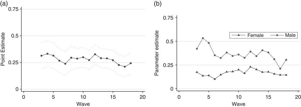
Fig. 6 Instrumental variables first stage: over time results Note: Point estimates of the effect of height on income are produced in separate, wave-specific regressions, using the specification corresponding to Columns 2, 4 and 6 of Table 4.
Instrumental Variable Results
Turning now to the second stage, we estimate linear probability models of Support for Conservative, where income has been fitted in the first stage using height as an instrumental variable. The first row of Table 5 reports the estimates. In the simplest specification controlling for only age, sex and region (Column 1), each additional £1,000 of annual income translates into a 2.4 percentage point increase in the probability of supporting the Conservative Party. This estimate slightly increases to 3.2 percentage points when we add additional controls in Column 2.Footnote 44
Table 5 Support for Conservatives: Second-Stage IV and OLS

Note: dependent variable is ‘supports Conservative Party’. The first row reports coefficients on income from second stage of 2SLS regressions; the second row reports coefficients on income from OLS regressions. Extended controls include: married, white, years of schooling, religion. Full models reported in the Appendix. Heteroskedasticity-robust standard errors, clustered by household. Statistical significance: *10%; **5%; ***1%.
Figure 7 offers suggestive evidence as to why the relationship between income and political preference is difficult to capture in the absence of an explicit identification strategy. Here we plot the propensity to support Conservatives on income, corresponding to the OLS specification, and the projection of income on height, corresponding to the IV specification. The latter curve is substantially steeper.Footnote 45
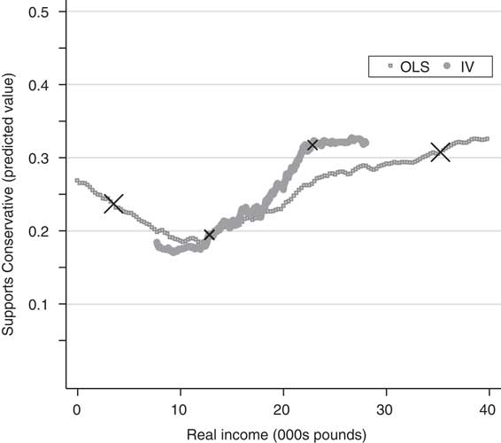
Fig. 7 Income and support for Conservatives Note: Running line smooth of ‘supports Conservative party’ on income and income projected on height, adjusted for age and gender. The Xs mark the 10th and 90th percentile of the income and predicted income distributions.
Table 5 provides parametric estimates of this relationship. The second row reports linear probability model estimates, regressing support for the Conservatives on income. Here, an additional £1,000 yields only a 0.2–0.3 percentage point higher probability of supporting the Conservatives (Columns 1 and 2). In contrast, the IV estimates in the first row of Columns 1 and 2 are an order of magnitude larger.
What should we make of these results? The first key point is the one that we have just seen: straightforward OLS estimates are close to zero (even as the model is saturated), while the IV estimates are substantially larger. Insofar as these results apply to other settings, estimates of the effect of income on right-leaning political preferences may be biased downwards, helping to explain the negligible or zero effects found in several other studies.
The second notable finding is that while our IV estimates dominate the OLS, they are not extremely large. Looking at our IV estimates in Figure 7, we see that income appears to have a fairly linear effect on preferences for the bulk of the sample. From our point estimates presented in Table 5, a £1,000 increase in income, which is 5.8 per cent of mean income, translates into a 3.2 percentage point increase in the propensity to support the Conservatives. At the same time, this estimate can only explain a small fraction of the variance in Conservative support, precisely because even in the 10th income percentile, predicted Conservative support is above 20 per cent, and in the 90th percentile it is just above 30 per cent. In this sense, our estimates indeed support the work of De La O and Rodden and Huber and Stanig,Footnote 46 among others, who probe alternative determinants of partisanship.
As with the reduced-form estimates reported above, the IV results suggest that income drives not simply conservative support but also a wide range of redistributive preferences. This can be seen the first row of Table 6, which reports regressions of support for various policy preferences on income, instrumented with height. The effect of income follows the pattern seen for Conservative support, with policy preferences turning against market intervention as income rises.Footnote 47 To interpret the substantive size of the effects, consider that the standard deviation of each outcome is approximately 1, and the standard deviation of income is approximately £14,000. Thus, for the proposition regarding private enterprise, a one standard deviation increase in income corresponds to about a 0.4 standard deviation increase in support for the proposition. As in the reduced form, the effect of income is strongest with respect to the statement that the government should provide jobs for all. Here, a one standard deviation increase in income corresponds roughly to a one standard deviation decrease in support for the statement. Finally, in Column 5 of Table 6 we see again that voting follows support, with each additional £1,000 yielding a 2.8 percentage point increase in voting Conservative. Again, in contrast to the OLS estimates (reported in the second row of Table 6), which display a near-zero effect of income on voting, the IV results are an order of magnitude larger.
Table 6 Policy Preferences and Voting Conservative in 2005 General Election
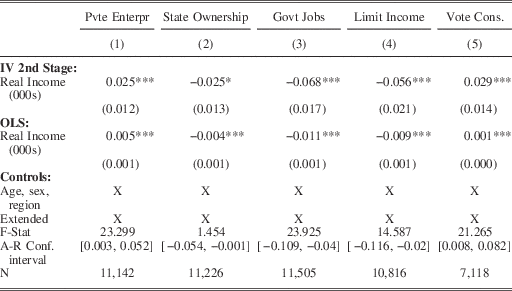
Note: dependent variables are (1) ‘Private enterprise is the best way to solve the UK’s economic problems’; (2) ‘Major public services and industries ought to be in state ownership’; (3) ‘It is the government’s responsibility to provide a job for everyone who wants one’; (4) ‘The government should place an upper limit on the amount of money that any one person can make’; and (5) ‘Voted for Conservative Party in 2005 General Election’. Each dependent variable indicates strength of support, ranging from −2 (strongly disagree) to 2 (strongly agree). The first row reports the second stage of 2SLS, the second row reports results from OLS regressions. Extended controls include: married, white, years of schooling, religion. Full models reported in the Appendix. Heteroskedasticity-robust standard errors, clustered by household. Statistical significance: *10%; **5%; ***1%.
Taken together, these results suggest that income positively influences not only support for conservative political parties, but also support for more conservative public policy positions.
IV Results: Over Time
The preceding instrumental variables results use Conservative support as measured in Wave 16, contemporaneous with the measurement of height. Do these results—for the whole sample, but also for the subsamples of men and women—hold over time? To correctly compare the income gradient over a period when real income is rising, Panel (a) of Figure 8 plots point estimates multiplied by a standard deviation of income in each wave. As with the reduced form and first stage, the consistency of the estimates over time is striking. The OLS estimates hover close to zero over the entire period; in contrast, the IV estimates are substantially larger. The IV results also suggest some intriguing patterns, although again confidence intervals are wide enough that we cannot reject a constant effect. Income’s effect on political support remains fairly consistent up through Wave 15 (1995), with a one standard deviation increase in income translating into a 30 percentage point increase in the propensity to support the Conservatives. We see some volatility in Waves 6–8, with the dip in the relationship between income and Conservative support falling most substantially in 1997, the year of Labour’s landslide victory. Wave 16 marks a sizeable increase in the income gradient; in the last three waves of the BHPS, a one standard deviation increase in income results in a nearly 50 percentage point increase in Conservative support. Due to the wide confidence intervals, these changes are merely suggestive, but these dips and rises are consistent with what we might expect from a voting model in which broad-based decline in support for a party increases the proportion of ideologues among its supporters, lowering the estimated income gradient. This explanation is confirmed by narrative evidence that the Conservative Party’s emphasis on ‘deep’ conservative convictions reduced it to core voters in the 1997 to 2005 period, but that after Cameron’s 2005 rise to power the party made successful appeals to a broader base.Footnote 48
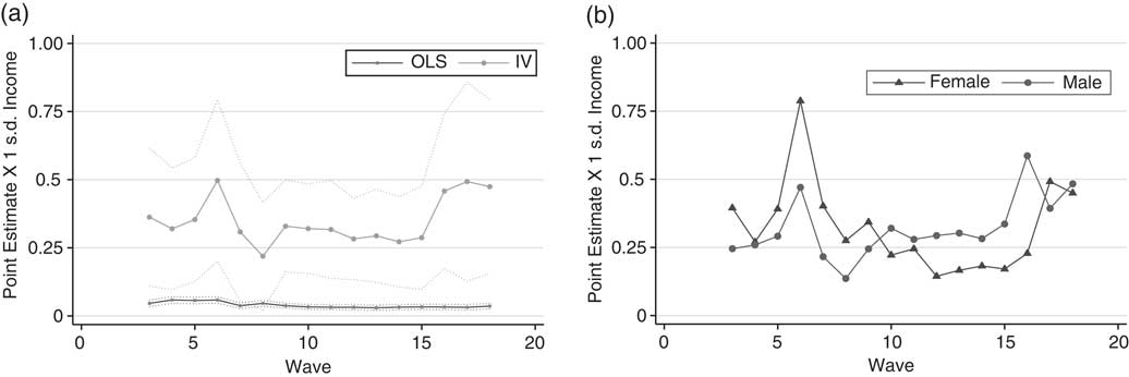
Fig. 8 Height and Conservative support over time: IV results Note: Point estimates and 95 per cent confidence intervals are produced in separate, wave-specific regressions, using the specification corresponding to Column 2 of Table 1. Panel (a) and (b): Effect of a standard deviation increase in income (by year; by year and sex) on Conservative support.
The results for Wave 16 broken down by gender are presented in Columns 8–11 of Table 5. For both sexes, we see the same patterns as in the whole sample: estimated IV effects are an order of magnitude larger than the OLS results. Whereas in the OLS, an additional £1,000 of income has almost no effect on Conservative support among women, in the IV specification it results in a 1.8–2.4 percentage point increase in propensity to support the Conservatives, although in the fullest specification that includes parents’ schooling the estimate for women becomes statistically insignificant. The point estimate of income’s effect is stronger for men. With mean incomes of £13,370 for women and £21,770 for men, this represents a steeper income gradient of political preference for men than for women: a 10 per cent increase in income results in a 2.3 to 3.4 percentage point increase in the probability of supporting the Conservatives for women, and a 7.8 to 8.2 percentage point increase among men.
Plotting the gendered estimates over time complicates this story. In the early waves of the panel, the income gradient for women dominates that for men until Wave 10, when this relationship flips. The differential between men and women peaks in Wave 16; by the last two years (2007–08) the estimates converge. Why men begin to exhibit a steeper income gradient of political preference starting in the early 2000s is somewhat puzzling. In a separate article, we study the political effects of a 2000 court case that altered the distribution of assets upon divorce and thereby shifted women’s expected income relative to men, but the results from that study do not suggest that the income gradient itself would shift.Footnote 49
The results over time should give us pause in interpreting the IV results for women and men in Columns 8–11 of Table 5. When plotted over time, Wave 16 is an outlier; for most of the period the male and female income gradients track each other fairly closely, and are statistically indistinguishable. In sum, while there is suggestive evidence that it was stronger for women in the 1990s and then stronger for men in the 2000s, with the genders converging by the end of the period, the extensively overlapping confidence intervals suggest that we cannot detect a substantial gender difference in income’s effect on political preferences.
Permanent versus Transitory Income
Finally, we return to the disjoint between theory and the bulk of empirical work on income and voting. Implicit in formal political economy models is the notion that permanent income generates political preferences; as Lind observes, however, most studies that examine effects on voting use a measure of current income.Footnote 50 For example, tests of egocentric/pocketbook voting typically ask whether an individual’s personal economic situation has improved, stayed the same, or worsened in the previous year. To probe whether transitory income shapes political preferences, we exploit the entire panel from 1991 to 2008 and regress support for the Conservative Party on income, including year dummies and individual fixed effects. Effectively, by differencing out average income, we can isolate the effects of short-term changes in income on political behavior.Footnote 51
To clarify what the fixed effects model captures, consider someone who earns an average of £10,000 a year over fifteen years. In one of those years, she receives £1,000 more than average. Does this make her more likely to support the Conservative party in that year, given that her permanent income is unchanged? Table 7 reports the results: precisely estimated near-zero effects, both in the whole sample and for women and men separately, suggesting that short-term fluctuations in income do not predict political preferences. Placed in conjunction with our earlier results, our finding is that it is permanent income, and not transitory income, that shapes political behavior.Footnote 52 The fact that most studies focus on the latter income measure may explain their varied findings (which may be sensitive to specification) and often small estimated effects.
Table 7 Fixed Effects: OLS

Note: linear probability model with individual fixed effects and year dummies; dependent variable is ‘supports Conservative Party’. Full models reported in the Appendix. Heteroskedasticity-robust standard errors, clustered by individual.
Statistical significance: *10%; **5%; ***1%.
There are important caveats to the fixed effects results, however. Although the within estimator pulls out some omitted variables bias from time-invariant characteristics that differ across individuals, it is open to two other problems. First, if annual fluctuation in income is small relative to baseline, this creates a problem akin to multicollinearity and may exacerbate attenuation bias. Secondly, problems with errors-in-variables are exacerbated in the fixed effects setting because we are focusing on within-individual variation over time. Potentially reasonable error structures that apply to income measurement can lead to perverse results, including attenuation bias and even sign reversal. Both concerns exist in our setting. For this reason, when pulling together our findings from the IV approach with the fixed effects results, we conclude that there is substantial evidence that permanent income shapes political preferences, but we do not find evidence that short-term fluctuations in income matter.
CONCLUSION
Does income drive political behavior? The notion that individuals’ economic standing shapes their political preferences enjoys a long intellectual lineage. Machiavelli advised his prince to abstain from touching citizens’ property, which could only serve to attract hatred and threaten the political order. By the era of classical liberalism, the notion that income shapes voting preferences was implicitly accepted. John Stuart Mill, for example, saw universal taxation as a necessary complement to the extension of the franchise, “as any power of voting possessed by [those who pay no taxes] is a severance of the power of control from the interest in its beneficial exercise”.Footnote 53 As we have argued, the idea that economic self-interest drives political behavior has remained at the core of modern political economy theory, yet the empirical evidence has remained mixed.
In this article we employ height as a lever to gain traction on this problem. Economic historians have long viewed height as a strong predictor of income, and anthropologists often use height to proxy for economic well-being when income measures are absent. Building on this tradition, we present two main findings. First, taller individuals are more likely to support the Conservative Party, support conservative policies and vote Conservative. Secondly, as an extension, we employ height as an instrumental variable for income, finding that each additional £1,000 of annual income translates into a 2–3 percentage point increase in the probability of supporting the Conservatives, and that income also drives political beliefs and voting in the same direction.
This article should be of particular interest to several groups of scholars. For example, the direct effect of height on voting will interest students of political behavior. In recent years, much has been made of the inability of economic fundamentals to effectively predict vote choice. As a result, analysts have increasingly shifted to analyzing Facebook, Twitter and other forms of social media, leveraging information on user connections to more effectively predict vote choice.Footnote 54 In contrast, we identify an ascriptive characteristic—height—that can be easily measured and which generates strong, clean predictions of voting behavior.
More generally, this article’s strategy of using height as a measure of economic well-being can be extended to a broad range of settings. Political scientists have decried the credibility of income measures in surveys that provide political information.Footnote 55 There are also many populations and associated large-sample surveys for which income variables do not even exist. For example, the Demographic and Health Surveys, which have been used to examine the effect of democracy on outcomes of interest in sub-Saharan Africa, elicit height but do not include an income module. In contrast, height is present in a number of major surveys that ask a broad range of political questions.Footnote 56
Finally, our results should be useful to studies that take positive political economy models to empirical data. The implications of such models often depend on the elasticity of voting behavior to income, which is rarely parameterized beyond assuming that income matters. This article fills this gap by providing one such estimate, which shows that income indeed drives political preferences. At the same time, our estimates leave much of the variation in partisanship unexplained, reinforcing the continued relevance of investigating non-economic sources of voting behavior.


