Models and forcing fields

The 2-D ice model used here is a derivative of the basic 2-D dynamic-thermodynamic model with a viscous-plastic ice rheology developed by Reference HiblerHibler (1979), and is similar to versions used in a variety of studies of sea-ice processes and sensitivities (e.g. Reference Walsh and ZwallyWalsh and Zwally, 1990; Reference Holland, Mysak, Manak and OberhuberHolland and others, 1993). Modifications include separate thermodynamic calculations for first-year ice, second-year ice. and multi-year ice (Reference Walsh and ZwallyWalsh and Zwally. 1990); an approximation of a thickness distribution for growth-rate calculations (Reference Walsh, Hibler and RossWalsh and others, 1985); and stability and fetch-adjusted turbulent fluxes (Reference Maslanik and KeyMaslanik and Key, 1995; Reference Ebert and CurryEbert and Curry, 1933). Albedo is estimated as a function of snow and ice thickness and melt-pond conditions (Reference Ebert and CurryEbert and Curry, 1993), with melt-pond albedo based on prescribed melt-pond depth and area that vary with ice type and duration of melt. A slab mixed-layer ocean is included that acts as a heat reservoir in areas with no ice cover. Radiathc fluxes, surface air temperatures, and winds are provided as external forcings as des-cribed below. Ocean flux and average annual geostrophic currents from an ice ocean model (Reference Hibler and BryanHibler and Bryan, 1987) are used as in Reference Flato and HiblerFlato and Hibler (1992). Precipitation is prescribed from climatology. The model domain includes the Arctic Ocean and adjacent seas (Fig. 1). Cell spacing of the Cartesian grid is 80 km. Eighteen year simulations were performed by cycling tw ice through the nine years of forcing data using a 12 hours time-step.

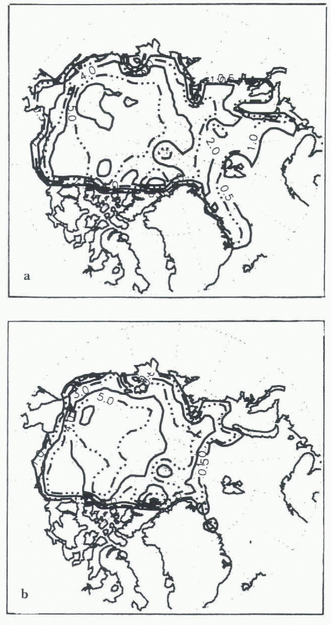
Fig. 1. Nine year mean ice thickness for March (a) and September (b) as simulated using a TO ice model and NCEP forcings.

The forcing fields were obtained from the National Center for Environmental Prediction (NCEP) National Center for Atmospheric Research (NCAR) Reanalysis Project for 1985-93 (Reference KalnayKalnay and others, 1996) and include downwelling longwave (F_L) and shortwave radiation (F_R), surface air temperatures (T_A), and sea-level pressures (SLP). Overall, the NCEP fields appear quite reasonable in terms of basic patterns and seasonal cycles. Monthly means averaged over the ice-model domain generally compare well with climatologies. However, F_R is greater than observations suggest, with a June mean at the orth Pole of 362 Wm⁻² . Also. T_A is greater than in the comparison data, mainly in spring. Overall, though, the NCEP data provide the best available suite of internally consistent and inter-annually varying forcings for the types of model experiments discussed here.

The NCEP data were mapped to the model grid using a Cressman distance-weighted interpolation. Geostrophic winds were calculated from the NCEP SLP. With these NCEP forcings, the ice model consistently produced an ice cover with realistic ice-adveciion patterns, but with an overestimate of summer melt when representative ice albedos were used. F_R was then reduced by a factor of 0.1 for a better match of the NCEP Fn with observations, and the NCEP temperatures for 15 May 30 June were replaced by climalo-logical air temperatures (Reference Crutcher and MeserveCrutcher and Meserve, 1970) to address the apparent positive bias in the NCEP air temperatures in spring. These adjustments are consistent with the effects of an underestimate in Arctic cloud fraction in late Spring and summer, which is seen in the NCEP data when compared to observations. The adjustments Io F_R and T_A (and the perturbation of these forcings) introduce some imbalance relative to each other and to the unchanged SEP fields, but this inconsistency is assumed of the insignificant for the interpretations used here. Using these revised forcings, the ice cover is simulated well throughout the year in the dynamic-thermodynamic (DT) control rim as discussed below, but with some remaining problems in the initial thermodynamic-only (TO) control run.

The stand-alone ice model ignores some other important features of the Arctic, including the effects of ocean dynamics on sea-ice anomalies and. in turn, main of the effects of ice transport and formation in modifying ocean saliniiy and temperature. An explicit ice-thickness distribution that includes ridging would also have an effect on the response of the ice pack io different climate scenarios (Reference Flato and HiblerFlato and Hibler, 1995), as is noted below in comparing the effects of the TO and DT thickness distributions. Details of regional atmosphere-ocean couplings, such as intensification of low-pressure systems and modifications of storm tracks, are also neglected. We expect, though, that the simulations here capture the basic patterns of sea-ice responses that could be expected from GCMs using this same basic type Of TO or DT ice treatment.

Experiment design

The experimental design consists ofa set of 2-D simulations in examine how ice extent and volume, simulated with and without ice transport, respond to F_L and T_A perturbations under the different atmospheric conditions represented by the daily varying forcings for 1985-93. The second part of the experiment considers how the relationships between ice transport and atmospheric forcings alfeet the interpretation of GCM climate-change simulations.

The suite of perturbed climate simulations using the 2-D ice model include: (Scenario 1) F_L x 1.03: Scenario 2) T_A+2.0°; (Scenario 3). F_L x 1.05 and T_A+ 2.0°. and To Separate 4) F_L x 1.05 and T_A + 2.0° . To separate the effects of inter-annually varying dynamic and thermodynamic forcings, an additional simulation (Scenario 5) was performed using the DT model with a nine year mean NCEP F_L and T_A “climatology” and inter-annually varying winds. Scenario 6 is the same as Scenario 1. but applied to the second of the two TO control runs, which is described below. The perturbations used are within the general range of mean changes predicted in doubled CO₂ scenarios, However, since the perturbations are applied uniformly, the effects of regional differences are not addressed.

The GCM scenarios investigated are present-day CO₂, and doubled CO₂ with separate climate-model runs using TO and DT ice.These coupled atmosphere ice simulations were obtained using the NCAR GENESIS (Global Environmental and Ecological Simulation of Interactive Systems) Earth system model Reference Pollard and ThompsonPollard and Thompson. 1994) . GENESIS version 1 is based on NCAR Community Climate Model (CCM1) and includes a cavitaling fluid DT ice model (Reference Flato and HiblerFlato and Hibler, 1992), a slab ocean, and a land-surface model. Version 2 of the global model performs relatively well for the Arctic (Reference Maslanik, McGinnis, Serrer, Dunn and Law-EvansMaslanik and others. 1996a), and includes aspects of CCM2 with various modifications and improvements to each Earth-system component. A principal difference between the model versions as used here is that the GENESIS version 1 simulations with dynamic sea ice were obtained using prescribed winds because of poorly simulated SLP fields, whereas the GENESIS version 2 results used interactively simulated winds. Model resolutions used are a spectral horizontal Atmospheric GCM (AGCM) grid of T31 (3.75°) latitude and longitude) with a 2 x 2O₂ surface model. GENESIS version 1 results are available for 1 x CO₂ and 2 x CO₂, scenarios with DT and TO ice (Reference Pollard and ThompsonPollard and Thompson, 1994). Version 2 runs have been completed for the two CO₂ scenarios with DT ice. and are in progress for the TO ice runs.

Ice-model control runs

Mean ice extent in March and September for the TO and DT ice-only model control runs (Figs 1 and 2) are similar (within 10%.} and reasonable, although overestimated in September. Magnitudes and inter-annual changes in iceextent (area covered by at least 15% ice) generally follow the time scries of SMMR and SSM/I derived ice coverage (Fig. 3). The DT ice thicknesses arc realistic, but the TO ice is too thick in the central and western Arctic due to localized apparent biases in the NCEP air temperatures. As seen in the DT results, the inclusion of ice dynamics reduces the effects of Such biases. Rather than further adjusting the forcings, a second TO control run (“Control 2”) was performed with the TO model tuned by adjusting albedo and minimum open-water fraction to yield a thinner initial ice cover. As shown later, the responses to perturbations depend on initial ice thickness. This second control run was therefore included to represent the TO model response given more realistic initial ice thicknesses.

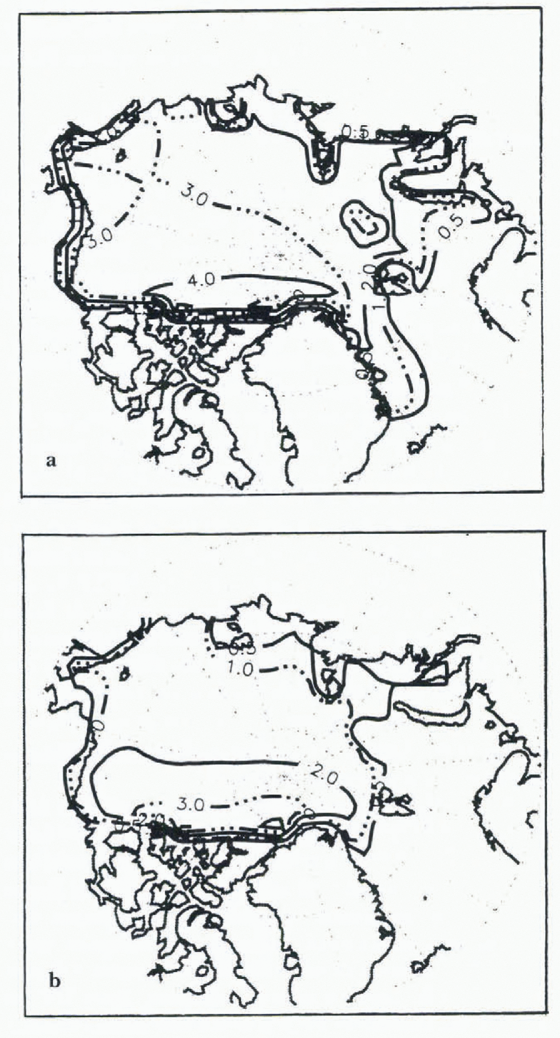
Fig. 2. Nine year mean ice thickness for March (a) and September (b) as simulated using a DT ice model and, NCEP forcings.

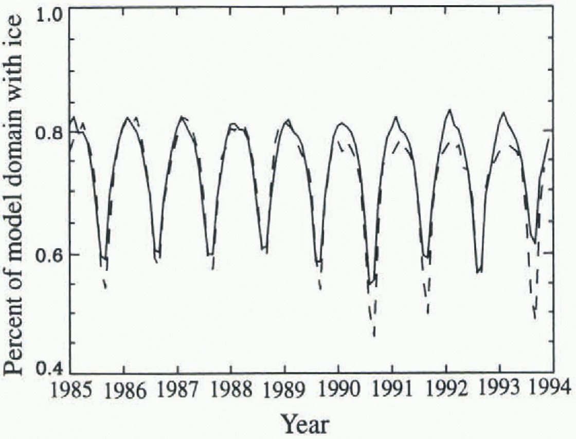
Fig. 3. Comparison of fraction of the Arctic Ocean and peripheral seas (the model domain in Fig. 1) covered by at least 15% infraction as simulated in the DT control run (solid line) and as mapped using SMMR and SSM/I data (dashed line) ( Reference Maslanik, Sorrcze and BarryMaslanik and others. 1996b).

Inter-annual variability and climate-change response as a function of ice treatment in the ice-only model

Inter-annual variability in fractional cover of ice in the Arctic Ocean is considerably greater in the DT runs (Fig. 4) than in the TO simulations, varying by a maximum in 1993 of 16% of the mean summer ice fraction for the DT control run. Ice Iiaciional coverage changes by < 1% in the TO Control 4% run and 4% in the TO Control 2 run for the nine year period. Ice volume (not shown, varies within ± 5% of the mean in the DT control run. except in 1993 when the summer anomaly is −8%. For the TO Control 1 volume, the maximum anomaly 1993 of −3% occurs in December 1993. with a variability of about 1% of the mean in other years, with similar variability in the Control 2 run. The DT simulation using inter-annually varying winds, but with the NCFP nine year climatology, yields a nearly identical variability, indicating that the inter-annual changes in ice cover are due mainly to ice-adveetion patterns rather than to short-term changes in air temperatures and radiative flux.

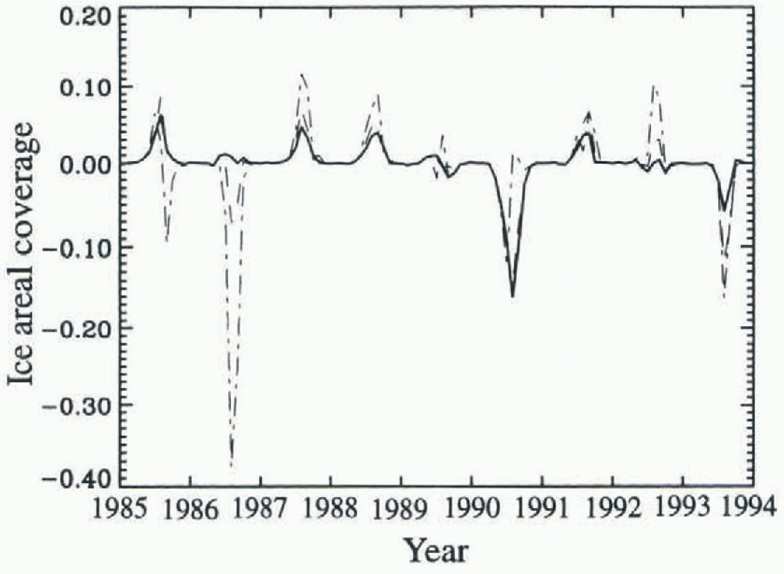
Fig. 4. Inter-annual variability in anomalies of sea-ice fractional coverage for the Arctic Ocean using the DT model. (control run is the solid line: climate scenario 1 is the dashed line: climate scenario 3 is the dash-dot line). Anomalies are the deviation of each individual monthly mean from the nine year mean for the control run and scenarios 1 and 3.

Interestingly the temporal variability and relative magnitudes Of these changes in ice fraction and ice volume under different climate-scenarios change in relation to patterns of large-scale ice transport. In the DT control run, minimum ice extent occurs in 1990, consistent with observations of ice extent (Reference Serreze, Maslanik, Key, Kokaly and RobinsonSerreze and others. 1995; Reference Maslanik, Sorrcze and BarryMaslanik and others. 1996b). However, when F_L and T_A are increased, the minimum ice fraction occurs in 1986 rather than 1990 (Fig. 4.) with a concurrent change in ice volume (Fig. 5). The explanation for this is that in 1986, winds favor a more southward ice margin by advecling ice into the Siberian, Chukchi, and Beaufort seas from the central Arctic. In 1990, reduced ice extent in summer is due primarily to northward advection of ice.

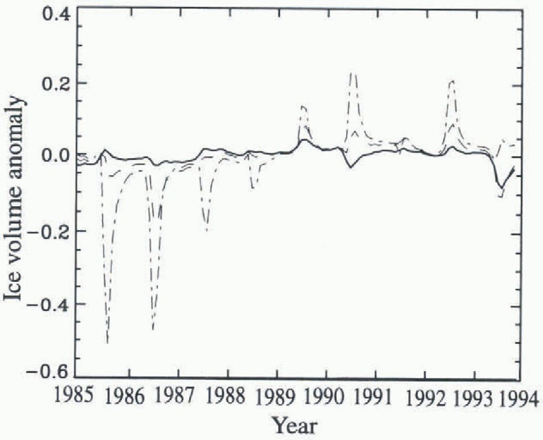
Fig. 5. Same eu Figure 4, but for inter-annual variability in anomalies of sea-ice volume (10⁴ km³).

Ice advection thus affects the climate response of the pack in 1986, and to a lesser degree in 1985, by placing ice in regions where melt is enhanced. In contrast, ice extenl in 1990 is less affected by enhanced melt since advection already produces a more northward ice margin, and the ice has been moved to a region of less melt. For small perturbations, the southward drift typical of 1986 might mask the effects on ice extent of additional melt, but for larger perturbations in T_A and F_l the southward ice advection is overwhelmed by the added melt, with the net result being a thinner ice pack and reduced ice extent. Iu short, changes in ice extent and volume are affected by a close coupling between melt and transport, where certain atmospheric circulation regimes might either enhance or reduce the response of the pack to changes in fluxes and air temperatures.

Overall response to climate change using TO vs DT ice

The decreases in nine year mean ice fractional coverage with increasing F_L and T_A are similar for the TO and DT runs, although the summer minimum TO ice extent is less sensitive than the DT ice extent to smaller perturbations. The thinner and slightly less extensive TO Control 2 ice pack (Scenario 6) is more sensitive than the thicker TO Clonlrol 1 ice. Ice fraction decreases by 22% and ice volume by 46%. As perturbations become larger, such as in Scenario 3, the TO model responds more than the DT model, with a 10% greater decrease in ice fraction.

Differences between the TO and DT runs are greater in terms of ice volume. As with ice extent, theTO simulations are more responsive to large perturbations. For example. the decrease in DT volume is slightly greater than the TO decrease for the Scenario 1 perturbation, but the DT ice volume is relatively insensitive to the extra Fr_L perturbation in Scenario 4 compared to Scenario 3 — ice volume is only 13% less in the Scenario 4 run. For TO however, the difference between Scenarios :', and 4 is 69%. Scenario 4 removes all but 4% of the September ice volume in the TO simulation, while 21% of the control volume remains in the DT simulation. The results are similar for mean annual ice volume, with the exception that the TO ice volumes are more sensitive than the DT ice volume to all the perturbation scenarios.

These patterns of differences in sensitivity reflect the nature of the ice cover simulated using a TO vs a DT model. In a TO simulation, the Arctic sea ice tends toward a more uniform thickness distribution. In contrast, the ice cover simulated using a DT model will typieally produce a bimodal thickness distribution that reflects ice thicknesses of 1-3 m over most of the basin, with much thicker ice Confined to the Canadian sector of the Arctic in response to the general wind patterns.With the TO Control 1 ice cover, the thickness distribution implies that a larger perturbation is required to reduce the ice thickness enough to produce large changes in ice extent. the DT ice cover, with its greater proportion of thinner ice, can respond more easily to smaller perturbations. A climate model with a TO ice model that produces an overly thick ice cover in a control run will be less sensitive to small changes in radiative fluxes or air temperature. The converse is true for a thin initial ice cover.

GCM results

The 2-D model results are relevant to the interpretation of global climate simulations. Reference Pollard and ThompsonPollard and Thompson (1994) summarize some of the aspects of including ice dynamics in their climate-change simulations, albeit with prescribed winds (the GENESIS version 1 runs discussed below). They find that the decrease in Arctic ice extent in a 2 x CO₂, scenario is affected only slightly if a DT ice model is used. However, as predicted by Reference Hibler and ACkleyHibler and Ackley (1983) in their comparison of the role of dynamics in simulating Antarctic ice. a larger effect occurs in the Antarctic due to the ability of the dynamic model to simulate a more realistic (less extensive) ice cover in the control run.

The 2-D model results discussed earlier suggest that the comparison of these GENESIS version 1 TO and DT runs for the Arctic should consider the spatial distribution of the ice pack in the 1 x CO₂ (control) case. In the GENESIS version 1 TO control run, ice thicknesses are too thin over much of the Arctic The GENESIS DT ice cover is more realistic in terms of thickness, but with thickest ice in the Siberian, central and cast Greenland Sea sectors of the Arctic rather than along the Canadian coast (Reference Pollard and ThompsonPollard and Thompson, 1994; Fig. 1).

Based on the 2-D model results, the relatively thin initial ice cover in the GENESIS TO run should accentuate the response to the 2 x CO₂ scenario. Since, in the DT run, ice is loo thick in the regions that show the greatest sensitivity in the stand-alone runs, the DT response to CO₂ doubling is probably underestimated. In both cases, the location of the remaining ice in the 2 x CO₂ scenario is confined to the central Arctic rather than the Canadian Arctic which, as noted above, could affect the ice-albedo feedback in the model by modifying the sensitivity of the ice pack to warming.

The GENESIS version 2 runs, using interactively-modeled winds, yield a more accurate spatial distribution of ice cover in the control DT run than was the case for inversion 1 simulation, even though prescribed winds were used in this earlier version 1 run. Changes in ice cover in the 2 x CO₂ scenario are similar to the 2-D ice model results, with ice extent decreasing in the Siberian Arctic and Greenland and Barents Seas. Perhaps due to the more realistic ice conditions, the resulting net decrease in ice extent is greater in the version 2 DT results than in the v.l simulations. The GENESIS version 2 TO runs have not yet been completed, but preliminary results from the 2 x CO, experiment suggest a greater response of the version 2 TO ice cover than was the case in the version 1 experiment. Initial ice thicknesses are probably similar to those m the version 1 ice cover, but with GENESIS version 2, ice is thickest near the Canadian Arctic rather than at the North Pole. This more realistic ice cover may be more sensitive to the 2 x CO₂ climate perturbation.