


1. Introduction
When a shock wave propagates in a confined space with non-uniform geometries, it undergoes complex reflection and diffraction phenomena. The processes involved are complicated to predict since they form a highly transient and non-uniform flow field. Multiple shock waves form when the incident shock encounters an abrupt area change, repeatedly interacting with each other, the walls and the background flow. The shock–structure interactions can cause extreme impulsive pressure loading, leading to equipment failure and, in some cases, catastrophic structural damage. Therefore, significant effort is invested in studying the transient phenomena of shock wave interactions to predict and prevent such detrimental consequences. A better understanding of the transient pressure fields associated with shock passage through an area change can also help solve various technological challenges encountered in designing jet engine ducts, mufflers, pressure relief valves, protective structures and more.
The problem of shock propagation through area increase is a fundamental problem in compressible fluid dynamics, and hence it has been studied extensively (e.g. Skews Reference Skews1967; Sloan & Nettleton Reference Sloan and Nettleton1975; Abe & Takayama Reference Abe and Takayama1990; Salas Reference Salas1993; Chang & Kim Reference Chang and Kim1995; Yu & Grönig Reference Yu and Grönig1996; Le, Moin & Kim Reference Le, Moin and Kim1997; Abate Reference Abate1999; Jiang, Onodera & Takayama Reference Jiang, Onodera and Takayama1999; Manna & Chakraborty Reference Manna and Chakraborty2005; Menina et al. Reference Menina, Saurel, Zereg and Houas2011). However, it remains poorly understood due to its complex nature and multiple shock–structure, shock–flow and shock–shock interactions. A significant number of studies have used both numerical and experimental methods to study the shock wave propagation and flow field evolution near an abrupt area expansion, many of them considered the classic case of a square cavity or a back-facing step (Hillier Reference Hillier1991; Igra et al. Reference Igra, Falcovitz, Reichenbach and Heilig1996; Abate & Shyy Reference Abate and Shyy2002; Mendoza & Bowersox Reference Mendoza and Bowersox2012; Soni et al. Reference Soni, Chaudhuri, Brahmi and Hadjadj2019). Nevertheless, being affected by multiple phenomena, it is hard to make general statements or predictions about the characteristics of the unsteady flow field. Many questions pertaining to the nature of the flow field evolution remain unanswered, and there is no explanation of the governing mechanism that eventually leads to its subsidence. As the shock wave propagates far downstream, it regains a constant velocity, which is referred to in this paper as a pseudo-steady-state velocity since the reflection phenomena behind it persist, albeit weaker.
When a shock wave propagates in long, uniform ducts, it tends to become a normal shock with a homogeneous front. As the normal shock encounters an area expansion, it conforms to it by refracting along the changing wall geometry, thus forming an expanding shock wave. A schematic of the shock wave evolution following an abrupt area expansion as it crosses a back-facing step is shown in figure 1. As the shock wave crosses the step expansion, it refracts across the corner, conforming to the area expansion (figure 1a). As it moves away from the entrance, the shock wave section that is far from the corner and close to the bottom wall remains normal. However, the section that diffracts across the corner becomes curved. As the shock wave continues to propagate away from the corner, larger sections of it become affected by the area expansion. Eventually, it reaches a critical point at which the entirety of the shock wave becomes curved. From that point on, the curved shock wave expands radially, continuously increasing its surface area (figure 1b). The incident shock wave position and shock decay in the expansion zone have been captured in detail by Sloan & Nettleton (Reference Sloan and Nettleton1975), Jiang et al. (Reference Jiang, Takayama, Babinsky and Meguro1997), Abate (Reference Abate1999), Abate & Shyy (Reference Abate and Shyy2002), Mendoza & Bowersox (Reference Mendoza and Bowersox2012), Murugan et al. (Reference Murugan, De, Dora and Das2012) and Dora et al. (Reference Dora, Murugan, De and Das2014). These studies show that the refraction process occurring near the step decreases shock speed and is accompanied by a reduction in pressure and velocity. The high-speed flow induced by the shock wave quickly forms a corner vortex (CV) downstream of the step. The vortex grows and moves further downstream as the incident shock wave propagates away from the corner. The temporal development of vortex trajectory near the entrance was studied by Chang & Kim (Reference Chang and Kim1995), Jiang et al. (Reference Jiang, Onodera and Takayama1999), Abate (Reference Abate1999) and Abate & Shyy (Reference Abate and Shyy2002). The CV is a short-lived starting process that quickly dissipates. However, before dissipation, it will interact with the reflected shocks near the expansion region, causing the formation of additional shock waves. Eventually, the fast flow induced by the shock wave will form a shear layer (SLr) downstream from the edge of the back-facing step.

Figure 1. A schematic representation of the flow field and incident shock wave evolution following an abrupt area expansion: (a) initial expansion near the corner where a portion of the normal shock undergoes radial expansion; (b) the whole incident shock wave expands radially; (c) the shock wave reflects off the top wall as regular reflection; (d) the shock wave transitions to Mach reflection with a triple point that propagates away from the wall.
When the expanding curved shock wave reaches the top wall of the larger cross-section region, it impinges on it as an oblique shock wave. The impinging shock interacts with the top wall at a shallow angle, thus forming a regular reflection (RR) pattern (figure 1c). The reflected shock wave propagating downwards interacts with the CV, resulting in the formation of a unique feature referred to as the ‘split reflected shock wave’ (Jiang et al. Reference Jiang, Takayama, Babinsky and Meguro1997), which consists of a shock wave moving perpendicularly to the flow direction, as well as a secondary shock wave that reflects off the vortex (Sun & Takayama Reference Sun and Takayama2003). As the incident shock wave continues to expand in the confined volume, the angle between it and the wall increases, and a transition occurs from RR to Mach reflection (MR) as illustrated in figure 1(d) (Chang & Kim Reference Chang and Kim1995; Ben-Dor Reference Ben-Dor2007). The transitions from RR $\rightarrow$MR and MR
 $\rightarrow$RR have been studied in detail for straight walls (Ben-Dor & Glass Reference Ben-Dor and Glass1979; Itoh, Okazaki & Itaya Reference Itoh, Okazaki and Itaya1981; Ben-Dor, Takayama & Dewey Reference Ben-Dor, Takayama and Dewey1987; Skews & Blitterswijk Reference Skews and Blitterswijk2011) as well as for convex–concave surfaces (Geva, Ram & Sadot Reference Geva, Ram and Sadot2013; Ram, Geva & Sadot Reference Ram, Geva and Sadot2015; Geva, Ram & Sadot Reference Geva, Ram and Sadot2018; Reshma et al. Reference Reshma, Vinoth, Rajesh and Ben-Dor2021). During the transition, a Mach stem (MS) forms near the wall, and the incident and reflected shock waves intersect at the triple point (TP). As the incident shock wave continues to propagate downstream, its curvature reduces, the height of the MS increases and the TP continuously moves away from the surface. Previous studies have thoroughly examined the processes occurring as the shock passes across the back-facing step. However, as the incident shock wave propagates away from the expansion region, the flow field becomes distinctively less complex and the flow near the expansion develops towards a steady state. To the best of our knowledge, no study has followed the subsequent shock wave propagation far downstream of the expansion region and examined how far the incident shock wave and reflection pattern remain affected by the expansion region.
Early in the research of shock wave propagation, it became apparent that predicting the motion of a shock wave undergoing an area change and interacting with walls of varying shapes poses a significant challenge. To efficiently estimate the temporal shape evolution and strength of the shock wave, a simplified Lagrangian framework known as geometrical shock dynamics (GSD) has been introduced (Whitham Reference Whitham1957, Reference Whitham1959, Reference Whitham1974). This approach simplifies the problem by reducing the complex equations of fluid dynamics to a more manageable set of geometrical relationships. The GSD solution is based on a method that involves breaking down the shock front into elementary ray tubes. By considering small changes in the ray tube area and neglecting the influence of the post-shock flow on the shock, a simple relationship called the  $A$-
$A$- $M$ rule is derived in the following form:
 \begin{equation} A=A_{0}\frac{f( M )}{f( M_{0} )},\end{equation}
where  $M$,
$M$,  $A$,
$A$,  $M_{0}$ and
  $A_{0}$ are the local Mach number, ray-tube area, initial Mach number and initial ray-tube area, respectively. The function
  $f(M)$ is given by
 \begin{equation} f( M )=\exp \left( -\int{\frac{M\lambda( M )}{M^2-1}}\, {\rm d} M \right),\end{equation}
where
 \begin{equation} \lambda( M )=\left( 1+\frac{2}{\gamma+1}\frac{1-\mu^2}{\mu} \right) \left(1+2\mu+\frac{1}{M^2} \right); \quad \mu^2=\frac{( \gamma-1 )M^2+2}{2\gamma M^2-(\gamma-1 )}, \end{equation}
where  $\gamma$ is the ratio of specific heat capacities.
Multiple algorithms have been developed in order to solve the propagation of the shock wave according to GSD (e.g. Schwendeman Reference Schwendeman1988, Reference Schwendeman1993; Apazidis & Lesser Reference Apazidis and Lesser1996; Aslam, Bdzil & Stewart Reference Aslam, Bdzil and Stewart1996; Schwendeman Reference Schwendeman1999; Noumir et al. Reference Noumir, Le Guilcher, Lardjane, Monneau and Sarrazin2015; Qiu, Liu & Eliasson Reference Qiu, Liu and Eliasson2016). GSD has been widely used to predict the evolution of shock waves in a plethora of cases that include: shock propagation across ramps (Henderson Reference Henderson1980; Itoh et al. Reference Itoh, Okazaki and Itaya1981; Henshaw, Smyth & Schwendeman Reference Henshaw, Smyth and Schwendeman1986), Shock focusing (Schwendeman & Whitham Reference Schwendeman and Whitham1987; Apazidis & Lesser Reference Apazidis and Lesser1996; Cates & Sturtevant Reference Cates and Sturtevant1997; Apazidis et al. Reference Apazidis, Lesser, Tillmark and Johansson2002; Qiu et al. Reference Qiu, Liu and Eliasson2016), shock expansion across corners (Bazhenova, Gvozdeva & Zhilin Reference Bazhenova, Gvozdeva and Zhilin1980; Skews Reference Skews2005; Ndebele & Skews Reference Ndebele and Skews2019b; Thethy et al. Reference Thethy, Haghdoost, Kirby, Seo, Nadolski, Zenker, Oevermann, Klein, Oberleithner and Edgington-Mitchell2022), shock passage in conduits of mild area change (Ndebele, Skews & Paton Reference Ndebele, Skews and Paton2017; Ndebele & Skews Reference Ndebele and Skews2019a), propagation of blast waves (Ridoux et al. Reference Ridoux, Lardjane, Monasse and Coulouvrat2020) and more. Surveying these studies reveals that although GSD has been widely used to assess shock propagation velocity and its shape in the immediate aftermath of shock structure interaction, it has not been employed to predict the evolution over longer periods. This limitation is attributed to the following reasons: (i) there is no correlation between shock propagation and the flow behind it, (ii) modelling shock reflection phenomena and associated shock–shock and shock–wall interactions is not feasible and (iii) the fundamental nature of GSD makes it less accurate in expanding regions where the shock strength diminishes. The aforementioned limitation has been addressed by Ridoux et al. (Reference Ridoux, Lardjane, Monasse and Coulouvrat2019), who introduced a correction for expanding geometries, such as in the diffraction of a weak shock over a convex wall. Although GSD provides a useful framework to study the shock front evolution it cannot yield a detailed description of the entire flow field. With recent advances in high-resolution numerical methods, many have turned to techniques such as large eddy simulation (LES) that can resolve shock propagation, reflections, shock–shock, shock–SLr and shock–turbulence interactions with high fidelity (e.g. Chaudhuri, Hadjadj & Chinnayya Reference Chaudhuri, Hadjadj and Chinnayya2011; Chaudhuri et al. Reference Chaudhuri, Hadjadj, Sadot and Ben-Dor2013; Vane & Lele Reference Vane and Lele2013; Pal, Roy & Halder Reference Pal, Roy and Halder2023). These allow to investigate the propagation of the shock waves in much more complex scenarios where simplified reduced-order techniques such as GSD are ineffective.
The current study aims to investigate the complex dynamics of the shock wave reflection patterns and flow fields by focusing on the evolution of the phenomena associated with an abrupt area change for an extended duration. We performed multiple experiments in a  $40\ {\rm mm}\times 40\ {\rm mm}$ square shock tube fitted with an unusually long 2 m test section to capture the flow field evolution over an extended duration and distances. The experiments were conducted in air (
 $\gamma =1.4$) with incident shock wave Mach numbers of 1.4 and 1.7. Varying cross-section expansion ratios were used in the test section, resulting in a 175 %–325 % increase in area. The extended test section enabled monitoring the evolution of the flow field for a duration longer than 10 ms. High-speed schlieren imaging and multiple high-speed pressure transducers were utilised to capture the flow field evolution post-expansion. This set-up allows for detailed spatiotemporal visualisation of the complex phenomena that occur close to the entrance of the expanded region, including the formation of a large vortex near the corner of the area expansion and its evolution into a steady SLr. As the incident shock wave moves away from the expansion region, the TP impinges, reflects off the top wall and propagates back towards the bottom wall. We have found that as the TP propagates downstream, it gets repeatedly reflected between the walls, forming a train of reflected shock waves. Every reflection of the TP creates an additional shock wave and extends the length of the shock train that follows the incident shock wave. The multiple reflected shocks cause significant pressure fluctuations, which persist for an extended duration following the arrival of the incident shock wave. Eventually, far enough behind the incident shock wave, the pressure fluctuations subside. The reflection pattern created behind the incident shock wave effectively divides the region into three parts: (i) the entrance region in which there is a strong SLr and unsteady velocity field; (ii) a steady-state region in which there are no strong shock waves; (iii) a highly transient region characterised by strong shock waves and pressure fluctuations.
The subsequent sections are structured as follows. First, we present the experimental and numerical methods (LES and GSD), followed by a detailed description of the short-time evolution close to the expansion region. The following section focuses on the shock reflection dynamics, TP trajectory and downstream evolution after the area expansion region. We have found that the evolution of the incident shock wave downstream of the abrupt expansion can be scaled using the expansion ratio and the shock wave pseudo-steady state velocity far downstream. The experimental observations are then compared with both LES and GSD, exploring the applicability of these techniques to the case of a sharp area expansion. Using the numerical simulations to extend our parameter space and developed a new simple constitutive equation to calculate the pseudo-steady-state incident shock velocity for both gradual and step expansion geometries. The results provide new insights into the physical mechanism that governs the dynamics of the shock front, which eventually evolves into a normal shock wave with uniform velocity.
2. Methodology
2.1. Experimental system
This study utilises high-speed imaging, pressure measurements and high-fidelity numerical simulations to investigate the flow field and shock reflection pattern that occur as a shock wave propagates downstream of an abrupt expansion. The experiments were conducted in the Transient Fluid Mechanics Laboratory (TFML) shock tube at the Technion-Israel Institute of Technology. A schematic of the shock tube and the geometry of the test section are shown in figure 2. The shock tube has a 3000 mm long, 52.5 mm inner diameter driver section and a 4080 mm long,  $40 \times 40$ mm
 $^2$ square cross-section driven section. These dimensions allow us to perform experiments with constant inlet properties to the test section for 6–8 ms, depending on the Mach number. The shock wave is formed by triggering a pneumatic fast-opening valve (ISTA KB-40) designed to open within 1–2 ms. The fast-opening valve produces repeatable shock waves with incident Mach numbers (
 $M$) ranging from 1.2 to 1.8, with less than 0.3 % variations between consecutive experiments (Ram et al. Reference Ram, Geva and Sadot2015). The shock tube is connected to a test section that is 2000 mm long and 40 mm wide, in which the flow undergoes an abrupt area change with a variable back-facing step of 30–90 mm. The shock wave enters the test section inlet from the square driven section with a height
  $h$ of 40 mm and expands across the back-facing step into the adjustable expanded region whose height
  $H$ has been preset between 70 and 130 mm as shown in figure 2(b). The test section is assembled from two 1000 mm long sections, fitted with two 40 mm thick clear acrylic windows that enable unobstructed optical accesses to record the flow field and shock wave evolution. Pressure is recorded in the shock tube from 26 flush-mounted transducers (PCB Piezo-electric 113B26 and PCB 482C amplifiers) using four oscilloscopes (LeCroy 3034Z) at 250 kHz. Two transducers are located 1000 mm apart upstream of the test section entrance to calculate the inlet incident shock wave Mach number. Twelve transducers are positioned along each of the test section walls. The shock tube facility is mounted on a movable platform, translating forwards or backwards using a geared stepper motor. This facilitates imaging the shock wave propagation at different locations along the test section without changing the optical set-up. The system operation is fully automated using an in-house LabVIEW controller, including the pressurisation process, triggering of the fast-opening valve and data acquisition. The imaging and the data acquisition systems are synchronised using an external timing box (Quantum composers 9400) triggered by the shock wave arrival at the first pressure transducer mounted before the test section.

Figure 2. (a) A schematic representation of the key components and layout of the shock tube. (b) The test section has a back-facing step geometry to facilitate an abrupt area expansion.
High-speed schlieren imaging is used as the primary diagnostic system in this study to visualise the shock waves and other flow features. Figure 3 shows a schematic diagram of the imaging set-up. An LED light (Thorlabs CWHL5-C1) is directed through a pinhole to reduce non-uniformity in the beam and collimated using a parabolic mirror (Edmund Optics #32-276-533) with an unobstructed diameter of 286 mm. The collimated beam is aligned using two flat optical mirrors so that the light propagates perpendicularly through the test section. The collimated beam is focused using a similar second parabolic mirror through an iris at its focal point. The iris opening is set to create a schlieren image sensitive enough to capture the density variations in the SLr that forms downstream of the back-facing step. The use of an iris provides uniform schlieren sensitivity for light deflections in all directions. An imaging lens is used to form the image of the test section at the plane of the camera sensor after being directed through a 2 $''$ 50:50 cube beamsplitter (Thorlabs BS031) to a second camera. Both cameras (Phantom V2640) are set at the same acquisition frequency but shifted in time with respect to each other by half the inter-frame time. By syncing the views of the two cameras, this configuration doubles the sampling rate of the schlieren imaging. This image acquisition system enables recording the flow field at a frequency of up to 140 kHz, depending on the field of view. Experiments performed with lower step heights require smaller imaging windows, thus enabling a faster acquisition rate. Table 1 provides the imaging configurations for the different step heights. The images captured by the two cameras are combined into one higher frame-rate video after they are calibrated and dewarped. A custom-made 1000 mm long calibration plate is used to correct the images at each imaging location and to accurately determine the location of the specific experiment field of view.

Figure 3. A schematic diagram illustrating the components and layout of the schlieren imaging system used in this study to visualise density variations and shock waves.
Table 1. Camera settings and region of interest based on step height ( $h=40$ mm).

Experiments were recorded at various downstream locations along the test section by translating the shock tube from  $x=0$ mm to
  $x=1860$ mm by increments of 220 mm. Owing to the highly repeatable nature of the shock wave reflection phenomena (Abate Reference Abate1999; Geva et al. Reference Geva, Ram and Sadot2013; Ram et al. Reference Ram, Geva and Sadot2015), this technique allows for the reconstruction of a complete visualisation of the evolution of the shock wave propagation along the entire test section without the need to realign the imaging optics. Hence, each experiment captures the shock wave in 25–80 frames, depending on the acquisition rate and
  $M$. Three experiments were performed at every location with varying timing to improve the temporal resolution further. In each experiment, the driver pressure was set to 20 and 25 bar, forming a repeatable shock wave with an incident
  $M$ of 1.4 and 1.7, respectively. The air in the driven section and the test section was kept at atmospheric conditions before the experiments as the end of the shock tube remained open. We have allowed for a long time (about 10 minutes) between experiments for the condition in the driven and test sections to re-equalise with the lab air. Consecutive experiments are run with a sufficient delay to ensure that the incident shock wave propagates into quiescent air with uniform atmospheric properties. The experiments are performed without an end wall to prevent a return of a reflected shock from the end of the test section to extend the experiment duration.
2.2. Large eddy simulations
To complement the experimental measurements and gain additional insights, a set of numerical simulations is performed by solving the unsteady three-dimensional (3-D) compressible Navier–Stokes equations using an in-house solver. The inviscid flux discretisation is performed using the low dispersion sixth-order Optimised Upwind Reconstruction Scheme (OURS6) of Chandravamsi & Frankel (Reference Chandravamsi and Frankel2024). The shock capturing is performed through the monotonicity preserving limiter of Suresh & Huynh (Reference Suresh and Huynh1997). The Harten, Lax and van Leer with contact (HLLC) approximate Riemann solver (Toro Reference Toro2019) is being used to compute the interface fluxes. The viscous flux terms are discretised using the sixth order Midpoint based Explicit Optimised scheme (ME6-Opti) of Chandravamsi & Frankel (Reference Chandravamsi and Frankel2024). The high order and high-frequency damping nature of the viscous scheme ensures odd-even decoupling free flow field and improved simulation stability. The time advancement is performed using the third-order Total Variation Diminishing (TVD) Runge–Kutta scheme detailed by Gottlieb & Shu (Reference Gottlieb and Shu1998). The inherent numerical dissipation of the discretisation algorithm in the high wave number range is being used to account for the sub-grid-scale stresses and act as a LES filter (Ahn, Lee & Mihaescu Reference Ahn, Lee and Mihaescu2021; Chandravamsi et al. Reference Chandravamsi, Chamarthi, Hoffmann and Frankel2023). This renders the current approach as implicit LES. The flow solver utilises curvilinear coordinate transformation and a multi-block approach to handle the present geometry, and it has been previously well-validated across a wide range of compressible flow test cases, as detailed in Chandravamsi et al. (Reference Chandravamsi, Chamarthi, Hoffmann and Frankel2023) and Kakumani et al. (Reference Kakumani, Chamarthi, Hoffmann and Frankel2023). To ensure free stream and vortex preservation properties, the metric terms corresponding to the coordinate transformation are computed consistently with the inviscid flux discretisation scheme.
The geometry and initial conditions of the problem were chosen based on the experimental set-up. The computational domain includes only the driven and test sections, excluding the driver sections. All the simulations were performed under a grid resolution of 120 million cells with an average of 3000 cells per metre. Grid clustering was employed near the wall and the entrance region of the test section with  $\Delta x_{min}=\Delta y_{min}=2\times 10^{-6}h$ in an attempt to capture the fine scales. Although the grid resolution employed is not fully sufficient to capture all the turbulent scales, the purpose of the present numerical simulations was restricted to accurately capturing the shock structure evolution and its downstream propagation. All the walls in the computational domain are imposed with the adiabatic wall boundary condition. At the entrance and exit of the geometry, non-reflecting sponge zones with zero gradient boundary conditions are employed to ensure no reflections enter the duct. We have verified that the use of wall boundary conditions, as opposed to periodic boundary conditions in the spanwise direction, has no significant impact on the dynamics of the shock structure evolution. Furthermore, given the nominally two-dimensional (2-D) dynamics of shock motion and reflection phenomena observed in experiments, we have performed all computations using half the span of the experimental set-up (20 mm) and imposed periodic boundary conditions in the spanwise direction. This helped us to reduce the computational domain size in the spanwise direction by half and double the grid resolution in the streamwise direction. The computations were carried out in parallel on four NVIDIA A100 GPU cards employing OpenACC directives (Chandrasekaran & Juckeland Reference Chandrasekaran and Juckeland2017) and Message Passing Interface (MPI).
2.3. Geometrical shock dynamics model
GSD is used to complement the experiments and the 3-D LES. As discussed in § 1, this model computes the Mach number of the shock front based on its instantaneous geometry and initial conditions through the  $A$-
$A$- $M$ rule (1.1). Several modifications have been proposed to the
  $A$-
$A$- $M$ rule since Whitham (Reference Whitham1957) original paper to enhance the model's accuracy (e.g. Oshima et al. Reference Oshima, Sugaya, Yamamoto and Totoki1965; Bazhenova et al. Reference Bazhenova, Gvozdeva and Zhilin1980; Best Reference Best1991; Sharma & Radha Reference Sharma and Radha1994; Ridoux et al. Reference Ridoux, Lardjane, Monasse and Coulouvrat2018).
To account for the inaccuracies of the Whitham (Reference Whitham1957) GSD model in low-Mach-number expansion regions, we employ the  $A$-
$A$- $M$ rule modification proposed by Ridoux et al. (Reference Ridoux, Lardjane, Monasse and Coulouvrat2019). This modification introduces a correction term that accounts for the transverse variation of the Mach number along the shock front in the expanding regions. The modified
  $A$-
$A$- $M$ rule in integral form, with the transverse correction term, empirically derived by Ridoux et al. (Reference Ridoux, Lardjane, Monasse and Coulouvrat2019) from the experimental data of Skews (Reference Skews1967), can be expressed as follows:
 \begin{equation} \underbrace{\log \left( \frac{A(t + \Delta t)}{A(t)} \right) + \int_{M(t)}^{M(t + \Delta t)} \frac{m \lambda(m)}{m^2 - 1} \, {\rm d} m}_{\textit{Whitham (1957) original model}} + \underbrace{\int_{t}^{t + \Delta t} H(\kappa) g(M) \left| \frac{\partial M}{\partial s} \right| {\rm d} t}_{\textit{Ridoux et al. (2019) correction term}} = 0, \end{equation}
where
 \begin{equation} g(M)=\frac{k \lambda(M)}{2}-\frac{2 M^2}{k(M^2-1)}, \quad \text{with } k=0.985, \end{equation}
and  $s$ represents the curvilinear abscissa along the shock front. The correction term is activated only in the expanding regions of the shock and is deactivated in the compressive regions based on the local curvature
  $\kappa$ of shock using the binary factor
  $H(\kappa )$, where
  $H(\kappa )$ is defined as
  $H(\kappa ) = 0$ if
  $\kappa \leq 0$ (non-expanding region) and
  $H(\kappa ) = 1$ if
  $\kappa > 0$ (expanding region).
To solve the above-mentioned  $A$-
$A$- $M$ relation numerically and advance the shock front in time, we employ the 2-D conservative numerical approach of Ridoux et al. (Reference Ridoux, Lardjane, Monasse and Coulouvrat2019). Their method eliminates the need to calculate the integrals shown in (2.1) from
  $t = 0$, and instead performs integration based on the shock front information available from the previous time step. The numerical scheme follows these steps. (a) At
  $t=0$, the shock front is initialised with a set of discrete grid points and a corresponding local initial Mach number. (b) The
  $A$-
$A$- $M$ rule (2.1) is used to estimate the local Mach number at each grid point. (c) The grid points are advanced along the direction normal to the shock front using the computed local Mach number. (d) To ensure that the shock remains normal to the boundaries at the walls, the straight line formed by the last two grid points on either end of the shock is enforced to be perpendicular to the wall at all times. (e) A regularisation procedure is applied to maintain appropriate grid resolution along the shock front, with grid points added or removed in expansion and compression regions, respectively, as described by Henshaw et al. (Reference Henshaw, Smyth and Schwendeman1986). The GSD solution is obtained by iterating steps (b)–(e). Time-stepping is performed using the Euler time integration satisfying the Courant–Friedrichs–Lewy (CFL) condition with a CFL number of less than 0.5 for all the calculations presented in this study. For a detailed description of the numerical method used to solve the modified GSD model, see Ridoux et al. (Reference Ridoux, Lardjane, Monasse and Coulouvrat2019).
3. Results
The following sections provide a detailed description of the evolution of the shock wave as it crosses the back-facing step into the larger cross-section region. Initially, schlieren images are used to track the expansion of the shock wave close to the inlet. As the shock reflection pattern transitions from RR to MR and the highly transient starting processes subside, the results assume a zoomed-out perspective and the evolution of the shock waves is tracked along the entire length of the test section. The velocities of the shock wave front along the top and bottom walls and of the TP are traced to show that similar trends persist between experiments performed with various inlet conditions and geometries. Finally, the experimental results and simulations (LES and GSD) are used to develop a constitutive scaling law for the shock velocity far downstream of the expansion region based on the inlet Mach number and expansion ratio.
3.1. Shock evolution near the back-facing step
Figure 4 shows a series of schlieren images recorded in an experiment performed with  $H=70$ mm and
  $M=1.7$, focusing on the initial expansion process as the shock wave passes the back-facing step. A recording of the experiment is presented as supplementary movie 1 is available at https://doi.org/10.1017/jfm.2024.814. The shock waves in figure 4 are marked by their order of appearance (
 $1^{\rm st}$,
  $2^{\rm nd}$) and their type: incident shock (IS) or reflected shock (RS). Figure 4(a) shows the
  $1^{\rm st}$IS as it exits the shock tube and propagates into the expanded region of the test section at
  $t=0$. Immediately after it crosses the back-facing step, the shock begins to diffract and remains normal to the surfaces. Subsequently, part of the shock front becomes curved, and a portion of the shock propagates in the lateral direction, as seen in figure 4(b) marked by ES (denoting an expanding shock wave). As the IS continues to propagate downstream and the expanding curved section moves away from the back-facing step corner, longer sections of the IS become affected and begin to curve (see figure 4c) until, eventually, the entire IS becomes a curved expanding shock wave. The passage of the IS across and away from the back-facing step corner induces fast flow behind it (221 m s
 $^{-1}$ for
  $M=1.7$). This incoming flow immediately detaches from the sharp corner, forming a strong CV that begins to convect downstream away from the step. The vortex becomes visible in figure 4(b), and as the shock wave propagates away from the corner, its size increases drastically, as seen in figures 4(c) and 4(d). The IS impinges on the top wall of the test section at about
  $t=0.13$ ms and is then reflected to form an RR configuration as seen in figure 4(d). The reflected shock associated with the IS is marked by
  $1^{\rm st}$RS.

Figure 4. Schlieren time series recorded with  $H=70$ mm and
  $M=1.7$ showing the evolution of the shock wave reflection patterns as the wave propagates across the sharp area expansion: (a)
  $t=0$ ms; (b)
  $t=0.03$ ms; (c)
  $t=0.07$ ms; (d)
  $t=0.13$ ms; (e)
  $t=0.21$ ms; (f)
  $t=0.37$ ms. IS, incident shock wave; ES, expanding shock wave; CV, corner vortex; RS, reflected shock wave; MS, Mach stem; TP, triple point; SL, slip line; SLr, shear layer.
As the IS moves downstream, the shock wave front naturally evolves to reduce its curvature, increasing the angle between the RS and the top wall of the test section. At a certain point, the angle between the IS and the surface becomes too large to support the RR, and a RR $\rightarrow$MR transition occurs. The precise critical angle of this RR
 $\rightarrow$MR transition is not fully resolved in the literature. However, it has been extensively studied in both pseudo-steady and highly transient cases (Ben-Dor Reference Ben-Dor2007; Geva et al. Reference Geva, Ram and Sadot2013). In the shown data set, the RR
 $\rightarrow$MR occurs roughly at
  $t=0.16$ ms (precise transition image is not shown). Figure 4(e) shows the MR just after its formation and highlights associated features, namely, The TP, MS and slip line (SL). At
  $t=0.15$ ms (not shown), the 1
 $^{\rm st}$ reflected shock wave (1
 $^{\rm st}$RS) hits the CV. The shock–vortex interaction reflects a shock wave back towards the top wall and creates a second shock wave that propagates radially outwards from the vortex. The newly formed shock wave is marked in figure 4(e) as 2
 $^{\rm nd}$IS, and propagates downstream behind the 1
 $^{\rm st}$IS. At
  $t=0.37$ ms (see figure 4f), the 2
 $^{\rm nd}$IS that expanded in the test section creates a second RR pattern, 2
 $^{\rm nd}$RS on both the top and bottom walls. The created shock wave pattern is highly asymmetric, and features such as the CV, the 2
 $^{\rm nd}$IS and 2
 $^{\rm nd}$RS quickly disappear. However, they lead to a rapid non-uniform flow field with pressure fluctuations. The pressure recordings and their relation to the shock wave evolution are discussed in detail in § 3.3.
Figure 5 depicts flow field evolution as the 1 $^{\rm st}$IS continues to propagate away from the back-facing step. As time passes, the strong shock waves and transients that formed following the initial shock diffraction begin to subside. Figure 5(a) shows an image taken at
  $t=0.51$ ms after the shock has entered the expanded region and the 1
 $^{\rm st}$IS reached
  $x\approx 4.5H$. Multiple shock–shock interactions have taken place by this time (see figure 6b). Figures 5(a) and 5(b) show that an apparent change begins to occur in the flow fields; the CV becomes more dispersed, and its shape becomes less distinct as it moves away from the corner and has already gone through multiple shock–vortex interactions. A SLr begins to form and becomes visible in figures 5(a) and 5(b), very close to the corner, and as the CV propagates downstream, it extends and becomes longer and more pronounces in figure 5(c–f). As the SLrs develop, standing shock waves (SS) appear to form, spanning between the SLr and the bottom wall. As the boundary layer develops on the wall, two distinct lambda shock configurations (
 $\lambda$S) are seen due to the shock wave–boundary layer interaction and the shock wave–SLr interaction. The lambda configuration remains mostly stationary, forming a standing oblique shock wave between the SLr and the boundary layer. After the disappearance of the CV, a re-circulation region (RC) forms above the SLr, covering almost the entire field of view (
 ${\sim }3.7H$). The reflections formed by the 1
 $^{\rm st}$IS and the 2
 $^{\rm nd}$IS propagate one after the other and begin to merge (see figure 5a) and are reflected to form a 3
 $^{\rm rd}$RS. The reflected shocks continue to reverberate vertically between the walls, and are still visible in figure 5(a–c). As the reflected shock waves repeatedly interact with the walls, the turbulent flow formed by the SLr and the boundary layers, they weaken and completely disappear. In this experiment, after approximately 1.3 ms, the highly transient features have subsided, and the flow near the entrance region reaches a steady state.

Figure 5. A series of schlieren images recorded in experiments performed with  $H=70$ mm and
  $M=1.7$ shows the later stages of reflection patterns as the shock wave propagates across the sharp area expansion: (a)
  $t=0.51$ ms; (b)
  $t=0.58$ ms; (c)
  $t=0.94$ ms; (d)
  $t=1.26$ ms; (e)
  $t=2.85$ ms; (f)
  $t=4.43$ ms. CV, corner vortex; RS, reflected shock wave; SLr, shear layer;
  $\lambda$S, lambda shock configuration; SS, standing shock wave; SBL, shock boundary layer.

Figure 6. A series of schlieren images recorded in experiments performed with  $H=70$ mm,
  $M=1.7$, showing the shock wave propagation downstream along the test sections. (a–c) Shock wave propagating in the first section (
 $x=0$ mm to
  $x=960$ mm). (f,g) Later times when the incident shock wave propagates in the second section (
 $x=1040$ mm to
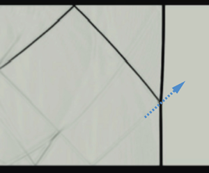
  $x=1860$ mm). The schematics provide an illustration of the TP local trajectory (dotted green line) and of the important velocities discussed in the following sections.
3.2. Downstream evolution of the shock wave
As the IS moves downstream from the entrance, the transient phenomena described previously tend to subside, and the IS and RS begin to converge. Figure 6 shows the propagation of the shock waves and the reflection patterns, recorded in experiments performed with  $H=70$ mm and
  $M=1.7$, as they reach various distances along the test section. These images have been generated by merging together multiple videos recorded at different positions along the test section. Each video corresponds to a particular streamwise location captured from a different experiment performed with the same inlet conditions. Since the incident shock wave propagates in a quiescent atmosphere, the experiments are highly repeatable, thus allowing the reconstruction of the instantaneous flow field over the entire test section. Whereas figures 6(a) and 6(b) depict a snapshot taken from a video recorded across the first location (from
  $x=0$ to
  $x=260$ mm), figure 6(g) required the use of images captured and combined from nine different locations. Schematic drawings are added to figures 6(c), 6(e) and 6(f) that show the different shock wave configurations at various streamwise locations. The velocity of the points at which the shock wave intersects the top wall and the bottom wall are marked by
  $V_{s,t}$ and
  $V_{s,b}$, respectively. The TP velocity is marked by
  $V_{TP}$, which has lateral and streamwise components
  $v_{TP}$ and
  $u_{TP}$ respectively. Videos of experiments and numerical simulation for
  $M=1.7$ and
  $H=70$ mm are provided as supplementary movies 1 and 2, respectively.
Figure 6(a), taken as the incident shock wave reaches  $x=128$ mm, depicts the shock reflection shortly after it has transitioned from RR to MR (RR
 $\leftrightarrow$MR). As the two incident shock waves move downstream, the 2
 $^{\rm nd}$IS propagates faster in the wake of the 1
 $^{\rm st}$IS, eventually catching up and merging with it. Figure 6(b) shows the 1
 $^{\rm st}$IS and 2
 $^{\rm nd}$IS as they get closer, just before they merge. Figure 6(c) shows one IS after merging. In addition, the 1
 $^{\rm st}$RS and 2
 $^{\rm nd}$RS also merge to form one RS. The RS seen in figure 6(c) reflects from the bottom wall, forming an RR pattern. It also shows that the reflected shock interacts with the SL formed by the MR, causing it to bend slightly. As the shock wave reflection transitions into MR, the TP moves toward the bottom wall, and the MS size increases. The TP propagates downwards until it impinges on the bottom wall and reflects towards the top wall, as seen in the shock reflection schematic of figure 6(c). The local trajectory of the TP is shown in the schematics by a dashed green line. Before the TP reaches the bottom wall, the IS size continuously diminishes until it completely disappears. Consequently, a new MS is formed as the TP now moves upwards, and the MS effectively begins to function as the IS. The IS
 $\leftrightarrow$MS reversal process repeats every time the TP impinges on one of the walls. Every TP impingement leads to the formation of a new RS that elongates as the IS moves away from the wall.
Figure 7 presents a schematic representation of the TP trajectory and the shock wave front evolution. The figure highlights the repeated IS $\leftrightarrow$MS transition and the changes that occur in the shock waves. The TP originates from the upper wall and follows the path of the incident shock wave as it propagates downwards. As the MS grows, the TP moves along the curved incident shock wave, which gradually begins to straighten. Consequently, the TP trajectory follows a curved path from the location of RR
 $\rightarrow$MR transition until it hits the bottom wall. After the first impingement, the newly formed MS and the accompanying TP propagate along the previous MS, which has taken up the role of IS and is relatively straight. Previous studies have recorded the evolution of the shock reflection pattern until the first impingement, after which the shock appears to be normal. However, analysis of the recordings shows that the shock front remains non-uniform and only becomes normal far downstream.

Figure 7. Illustration of the development of TP trajectory as the shock wave propagates downstream.
An oblique shock train forms behind the IS as seen in figure 6(d–g). When the incident shock propagates further downstream, every TP reflection leads to the formation of additional oblique shock waves. The oblique shock waves also propagate downstream but are slower than the IS, thus extending the length of the shock train. They also slow down and weaken, as seen in figure 6(e). As the distance between the reflections of the oblique shocks increases, the shock train widens. The tail of the shock train becomes a horizontally moving lateral shock wave that repeatedly interacts with the walls and the induced turbulent flow. The repeated interactions lead to its decay until it is no longer visible. Figure 6 shows that initially, the IS front does not propagate with a uniform velocity; however, as it moves downstream, it eventually becomes uniform. It is currently uncertain at which point downstream the shock becomes completely normal again after the expansion and what the mechanisms that govern it are. To provide new insights into the governing processes, the subsequent section tracks the TP trajectory and the shock front velocities far downstream in high temporal and spatial resolution.
3.3. Pressure field evolution downstream
Figure 8 presents eight sets of pressure profiles recorded in various  $x$ coordinates, at
  $H=70$ mm and
  $M=1.7$, obtained from pressure transducers flush mounted opposite to each other on the top and bottom walls. The locations of each pressure transducer couple are indicated in the figures. The pressure transducers located along the top wall are plotted in blue, whereas those along the bottom are plotted in orange.

Figure 8. Pressure profiles recorded at eight locations along the test section for  $H=70$ mm,
  $M=1.7$. Each figure shows two pressure profiles recorded at the same
  $x$ location, where the pressure transducers are flush mounted on opposite walls. The blue and orange lines represent top and bottom pressure transducer recordings, respectively. We set
  $t=0$ when the incident shock wave reaches the back-facing step corner.
Figure 8(a) shows the pressure at  $x=160$ mm, i.e.
  ${\sim }2.3H$ downstream of the back-facing step. Located fairly close to the step, the pressure profile exhibits a significant pressure drop occurring shortly after the arrival of the expanding shock wave. Located in a region of strong shear, recirculating flow and multiple standing shocks, the flow in this region remains highly unsteady for the entirety of the experimental duration. As described in previous sections, a more uniform shock front develops as it moves away from the back-facing step and the pressure profile tends towards a more distinct step function shape. The pressure transducers located at
  $x=475$ mm, shown in figure 8(c) do not show any distinct pressure drop as they are located away from the step and beyond the recirculating flow region. However, in accordance with the description presented in previous sections, the pressure profiles show that even far downstream of the step, the pressure behind the first pressure jump is followed by significant pressure fluctuations. These pressure fluctuations are caused by the reflected shock train that travels downstream behind the shock front. When the shock front propagates downstream and becomes more uniform, the amplitude of these fluctuations reduces. This feature is highlighted by the insets in figures 8(d) and 8(h) showing magnified images of the pressure profiles following the arrival of the shock front. A comparison of the two insets shows that the pressure fluctuations amplitude decreases, and the pressure behind the shock front becomes more uniform. However, comparing the different downstream locations shown in figure 8, it is evident that the number of reverberations increases as the shock propagates downstream. Comparing the pressure profiles with the spatial evolution shown in figure 6, as the shock train that follows the incident shock wave length breaks down, the amplitude of the fluctuations shown in figure 8 reduces. As the shock front propagates further downstream, the unsteady period exhibits smaller amplitude fluctuations but extends. For example, the pressures recorded at
  $x=685$ mm show significant sharp pressure jumps for
  $\sim$2.5 ms, however at
  $x=1464$ mm, pressure jumps, albeit weaker, persist for longer than 4.5 ms (when the experiment ends). Finally, also in accordance with the discussion presented in the previous sections, it should be noted that the pressure profiles on the top and bottom walls show pressure fluctuations that are out of phase. Depending on the response time of the system, the out-of-phase pressure fluctuation can cause structural vibrations and non-uniform side loading.
3.4. Triple point trajectory and incident shock wave velocity
Figure 6(a) shows that shortly after its formation, the MS propagates far behind the IS. However, figure 6(b) shows that about 0.22 ms later, the MS has moved in front of the IS. Between figures 6(b) and 6(c), the TP reflects from the bottom wall, an IS $\leftrightarrow$MS transition occurs, and in figure 6(c) the MS has moved ahead again. As the shock wave propagates downstream, this relative shift between the top and bottom parts of the shock wave repeats, showing that they are propagating with a non-uniform velocity. As mentioned previously, each impingement of the TP on a wall leads to an additional IS
 $\leftrightarrow$MS reversal process. Hence, to simplify the analysis, the following text focuses on three velocities: the velocities of the two intersections of the shock front with the top and bottom walls and that of the TP.
Figure 9 presents measurements obtained by tracking the TP and the top and bottom intersections of the shock front and the walls. The results are plotted from the moment the TP forms until it reaches  $x=1860$ mm. The experimental results presented in figure 9 were performed at
  $M=1.4$ (figure 9a–c) and
  $M=1.7$ (figure 9d–f) for
  $H=70$ mm, 100 mm and 130 mm. Videos were recorded at nine regions along the tunnel to compile the evolution of the shock wave along the whole test section. The TP spatial tracking is plotted in the top panels of figure 9. The bottom panels of figure 9 present the streamwise velocities measured from tracking the three locations along the incident shock wave, namely,
  $V_{s,t}$ (blue),
  $V_{s,b}$ (red) and
  $u_{TP}$ (orange). An overlap of
  $\sim$20 mm is kept between each imaging location to ensure spatial continuity of the data. The TP trajectory shown in the top panels of figure 9 shows that the distance between the locations at which the TP impinges on the top and bottom walls varies with
  $H$. The impingement locations on the bottom and top walls are highlighted on both panels in blue and orange vertical strips, respectively.

Figure 9. Experimental results obtained by tracking the TP trajectory and the top and bottom intersections of the shock front and the walls showing their streamwise velocities plotted vs  $x$: (a)
  $H=70$ mm,
  $M=1.4$; (b)
  $H=100$ mm,
  $M=1.4$; (c)
  $H=130$ mm,
  $M=1.4$; (d)
  $H=70$ mm,
  $M=1.7$; (e)
  $H=100$ mm,
  $M=1.7$; (f)
  $H=130$ mm,
  $M=1.7$. The top panels show the spatial locations of the TP (
 $y=0$ is located at the top wall where the TP forms), whereas the bottom panels show the streamwise velocities of the TP,
  $u_{TP}$, and the top and bottom intersection of the shock front with the walls,
  $V_{s,t}$ and
  $V_{s,b}$, respectively. The blue and orange vertical bars show the location of TP impingement on the bottom and top walls, respectively.
The plots of TP trajectories plotted for various  $M$ and
  $H$ in figure 9 further affirms that following its inception, the TP initially follows a curved trajectory along the expanding incident shock wave. The subsequent TP trajectories appear to be almost linear as the TP moves back along the MS of the previous reflection. It is also evident that, an increase in the expanded area height,
  $H$, leads to longer periods between subsequent TP impingement, whereas increasing the inlet incident Mach number,
  $M$, decreases it. It should be noted that the trajectory of the TP is incomplete, as there is a region of 125 mm gap between the two test section windows that cannot be filmed.
As shown in figure 4, when the shock wave propagates into the expanded section, it diffracts across the back-facing step corner, resulting in a significant velocity reduction, which is evident for all cases in figure 9. Previous studies, e.g. Jiang et al. (Reference Jiang, Takayama, Babinsky and Meguro1997) and Abate (Reference Abate1999), showed that while the section of the shock wave near the corner expands and impinges on the top wall as an oblique shock, the part that moves along the bottom straight wall decays while remaining normal to it. As the oblique shock impinges on the top wall and transitions to MR, its velocity near the wall,  $V_{s,t}$, is significantly higher than its velocity near the bottom wall,
  $V_{s,b}$. However, as seen in figure 9 both continue to decay. At the same time, when the TP moves along the curved incident shock wave, its velocity diminishes, conforming to the local velocity of the shock ahead. However, due to the compression facilitated by the reflected shock wave, the TP causes an increase in the local shock velocity. This effect is recorded vividly as the TP impinges on the bottom wall, where it converges with the IS and significantly accelerates as it reflects off the wall. Figure 9 shows that, as the TP propagates away from the bottom wall,
  $V_{s,b}$ begins to decrease again. At the same time,
  $V_{s,t}$ continues to decrease until the TP reaches the top wall and reflects off it. As this occurs,
  $V_{s,t}$ sharply increases but then similarly decreases as the TP propagates away. This process is repeated with every reverberation of the TP. Moving repeatedly between the top and bottom walls,
  $u_{TP}$ always lies between
  $V_{s,t}$ and
  $V_{s,b}$. Each consecutive reflection of the TP induces a smaller velocity increase. Figure 9(a), for example, highlights the first five reflections (marked with arrows, I–V); afterward, the velocity of all three seems to converge, reaching a pseudo-steady velocity, which we labelled as
  $u_{TPss}$ in subsequent sections.
3.5. Similarity and scaling
The six cases shown in figure 9 suggest that the trends discussed in the previous section persist when changing  $H$ and
  $M$. The distinction between the cases depends on the experimental conditions: (a) for a given
  $M$, increasing
  $H$ will increase the time between the TP impingement on the walls and decreases
  $u_{TPss}$; (b) for a given
  $H$, increasing
  $M$ will decrease the time between the TP impingement on the walls and increase
  $u_{TPss}$.
Using these observations, we were able to scale the results shown in figure 9 and have re-plotted the TP trajectories and streamwise velocities,  $u_{TP}$ in a non-dimensional form which is presented in figure 10. The test section height
  $H$ is used to normalise the TP spatial positions in both
  $x$ and
  $y$ directions. The results are shown in the upper panel of figure 10 for
  $M=1.4$ and
  $M=1.7$. The lower panel in figure 10 shows that
  $u_{TP}$ can also be normalised using the pseudo-steady-state streamwise TP velocity,
  $u_{TPss}$, which is also the normal shock wave velocity far downstream of the expansion. Although not shown here,
  $V_{s,b}$ and
  $V_{s,t}$ also converge in the normalised plots since the corresponding velocities equalise every time the TP impinges on a wall. Although figure 10 shows that the TP trajectories and velocities collapse for a given
  $M$, the corresponding scaling between various
  $M$ remains unknown. The non-dimensional plots provide a tool to predict the distance required to reach a normal uniform shock front. In these figures, the shock becomes normal after
  ${\sim }15H$ for
  $M=1.4$ and
  ${\sim }17H$, for
  $M=1.7$. Note that for
  $M=1.7$ and
  $H=130$ mm, the shock front does not reach a steady velocity even 2 m downstream of the step expansion. To the best of the authors’ knowledge, there is no method to predict
  $u_{TPss}$ given the
  $H/h$ and
  $M$.
$M$.

Figure 10. Normalised TP trajectories and velocities for all test cases. The spatial dimensions are normalised by the test section height  $H$, and the velocities are normalised by the TP velocity in the steady state
  $u_{TPss}$.
3.6. Comparing the experiments with LES and GSD
A survey of previous studies on shock–structure interaction presented in § 1 suggests that LES numerical simulations and GSD are two techniques that can potentially predict  $u_{TPss}$ for various
  $M$ and
  $H/h$. Figure 11 compares experiments with LES and GSD for two fundamentally different geometries in which the shock wave enters the expansion region at
  $M=1.7$ and propagates through an expansion of
  $H/h=1.75$. The first case presented in figure 11(a) examines a smooth and gradual shock expansion over a fifth-order polynomial spanning 15 step heights. The second case presented in figure 11(b) considers the case of the sharp area expansion, which is described in the previous sections. These provide us with the means to assess the applicability of each technique in predicting the downstream behaviour of the shock wave.

Figure 11. (a) A comparison between experiments, LES and GSD results for the case of a gradual expansion for  $M=1.7$ and
  $H=100$ mm along a fifth-order polynomial curve with a length of 15 step heights. (b) A comparison between experiments, LES and GSD results for a step expansion for
  $M=1.7$ and
  $H=100$ mm. The shock fronts are extracted from the snapshots and overlaid in the bottom panels of (a) and (b).
Figure 11(a) displays a comparison of four snapshots taken at different times showing the advancing shock locations along the gradual expansion. The numerical schlieren results from LES (computed as the magnitude of the density gradient vector) and the solution for the shock front from GSD are presented below the experimental results. In this case, there are no reflections, and the only effect of the expansion is a slight curving of the shock front. As the shock wave reaches the end of the expansion seen in time  $t=1.166$ ms, it has reverted back into a normal shock and moves with a uniform velocity. The shock fronts extracted from all three sets of results are overlaid at the bottom panel and show excellent agreement. GSD is well suited for the case of a gradual expansion without reflections where the effects of flow features behind the shock front are not significant. Hence, both GSD and LES provide a good estimate for the shock propagation downstream of the expansion region. Figure 11(b) presents a comparison between experiments, LES and GSD for the step expansion case at five downstream locations. First, this figure shows that the complex nature of the flow field is well resolved by the LES simulation, including the incident shock wave, reflected shocks, and subsequent shock interaction with the flow near the entrance region. Some differences are seen close to the back-facing step at later times due to the formation of a highly turbulent SLr. In accordance with previous studies (e.g. Bazhenova et al. Reference Bazhenova, Gvozdeva and Zhilin1980; Ridoux et al. Reference Ridoux, Lardjane, Monasse and Coulouvrat2019), GSD properly captures the shock diffraction across the back-facing step (
 $t=0.052$ ms and
  $t=0.122$ ms). However, the results shown in figure 11(b) show that since GSD cannot predict any of the flow features behind the shock front, it begins to deviate from the experiments and LES after the formation of MR (see
  $t=0.310$ ms). The shock fronts overlay at the bottom panel of figure 11(b) shows that as the shock continues to propagate downstream, GSD significantly overestimates the propagation of the shock front.
Figures 12(a) and 12(b) show a qualitative comparison between the normalised TP trajectory and velocity presented in figure 10(b) and those obtained from the LES simulations for  $M=1.7$ and
  $H=100$ mm. This figure demonstrates that the numerical simulation accurately predicts the propagation of the TP and its velocity. The good quantitative and qualitative agreement between experiments and computations in figures 11(b) and 12 provides confidence that the LES simulations can be reliably used to increase the parameter space for the step case, allowing us to find the dependency of
  $u_{TPss}$ on
  $M$ and
  $H$.
$H$.

Figure 12. A comparison between normalised (a) TP trajectories and (b) TP velocities obtained from three experiments with various  $H$ and the normalised LES results performed for
  $M=1.7$ and
  $H=100$ mm.
3.7. Predicting the steady-state velocity of the shock wave far downstream
To extend the results presented previously, we have performed a series of numerical simulations for both gradual and step expansion with 48 different parameter configurations each, ranging from  $H/h=1$ (no step) to
  $H/h=5$ and for
  $M=1.1$ to
  $M=1.8$. All the simulations were run until the shock front became normal downstream of the expansion. In addition, we have computed the downstream velocity of the shock front from GSD for both cases. Figure 13(a) shows the steady-state downstream shock front Mach number
  $M_{ss}$ plotted against the inlet Mach number after subtracting 1 from both for ease of analysis. Similarly, the steady-state streamwise TP Mach numbers
  $M_{TPss}$, which are also the steady-state incident Mach numbers far downstream,
  $M_{ss}$, are plotted in figure 13(c). The
  $M_{TPss}$ experimental values for the step expansion acquired from figure 9 are also overlaid on figure 13(c). In both cases, the results show that for the Mach numbers and expansion ratios simulated here, the relation between the inlet and downstream shock velocities can be approximated by fitting linear trend lines. The results of the linear fitting to the computational fluid dynamics (CFD) are plotted in figures 13(a) and 13(c) with solid lines and with dashed lines for GSD. The slopes of the linear fits shown in figures 13(a) and 13(c),
  $d(M_{TPss}-1)/d(M-1)$, are plotted in figures 13(b) and 13(d), respectively, against test section expansion ratios,
  $H/h$. Fitting a power law to the slopes (also shown in a log–log plot in the inset) provides a power of
  $-$0.42 for the case of a gradual expansion and
  $-$0.48 for the case of a step expansion from the CFD data. As discussed in the previous section, GSD provides a very good estimation for the shock front velocity downstream of a gradual expansion, as is evident in figure 13(b). However, the GSD results for the step expansion show a clear divergence as the
  $H/h$ increases. Nevertheless, in the current parameter space, GSD only overestimates the shock Mach number downstream by less than 6 % in relation to the CFD. The largest disparity for
  $H/h=5$ and
  $M=1.8$ where the shock downstream velocity is estimated to be 1.38 and 1.46 from the numerical simulation and GSD, respectively. Using the results shown in figures 13(b) and 13(c), we propose a new approximate method to predict the downstream shock velocity for both cases as
 \begin{equation} M_{ \it ss}\approx\left(\frac{H}{h}\right)^{n}(M-1)+1,\end{equation}
where  $n=-0.42$ for gradual expansion and
  $n=-0.48$ for the step expansion case. One should note that these coefficients should be considered as appropriate empirical approximations only for the range of parameters presented in figure 13. Using the non-dimensional TP velocities shown in figure 10 and (3.1) one can now adequately predict the evolution of the incident shock wave propagating downstream of the sharp expansion, relying only on inlet Mach number and test section height.

Figure 13. (a) Comparison of numerical and GSD estimates of the steady-state Mach number ( $M_{ss}-1$) vs inlet
  $M-1$ for the gradual expansion cases at various
  $H/h$ and
  $M$. (b) Power-law fitting to the linear slopes of the lines shown in (a) plotted against
  $H/h$. (c) Comparison of numerical and GSD estimates of the steady-state TP Mach number (
 $M_{TPss}-1$) vs inlet
  $M-1$ for the step expansion cases at various
  $H/h$ and
  $M$. (d) Power-law fitting to the linear slopes of the lines shown in (c) plotted against
  $H/h$. The insets in (b) and (d) show the power-law in log–log plots.
4. Summary and discussion
A complex and highly transient flow field develops when a normal shock wave propagates across a sharp area expansion. Multiple reflections form as the incident shock wave refracts across the corner, impinging on the wall of the expanded region, initially reflecting in a RR pattern before transitioning into a MR. Initially, as the shock propagates into the expanded region, its velocity decreases rapidly and multiple shock reflections are formed. The propagation of the shock wave near the expansion region is characterised by highly transient flow where numerous shock–shock, shock–wall and shock–vortex interactions occur. These interactions cause the shock velocity to fluctuate significantly for an extended duration as it propagates away from the corner. As the shock front continues to propagate downstream, it evolves to form a steady normal shock with a constant velocity. The following sections discuss new observations and insights that can be derived based on the results we have presented previously.
4.1. The governing mechanism of transient shock reflection decay
The process by which the normal shock front attains a uniform velocity is governed by the dynamics of the TP. Initially, the shock velocity varies significantly due to its highly non-uniform expansion. The shock propagates as a normal decaying shock wave at the bottom wall but impinges as an oblique shock at a shallow angle on the top wall. As it propagates downstream and undergoes RR $\rightarrow$MR transition, a normal accelerated MS is formed and increases in length as the TP propagates away from the wall. By the time at which the TP impinges on the bottom wall, the MS spans the entire cross-section of the expanded region. However, the recordings shown in figure 6 and the velocity measurements presented in figure 9 reveal that its velocity remains non-uniform. As the TP propagates away from the wall, the velocity of the foot of the MS decays. The TP reflects off the wall, reversing the direction of its propagation, forming a new inverted MR. The reflection process leads to the formation of a new MS that propagates faster. As the TP moves away from the wall, this new MS begins to slow down, but by the time the TP reflects off the top wall and returns, it does not decay to the same velocity it had prior to the reflection. This process repeats itself numerous times as the TP reverberates between the top and bottom walls, undergoing successive acceleration and deceleration cycles with each reflection. However, every TP reflection leads to a smaller velocity increase, eventually settling to a steady-state velocity. This process of TP reverberations across the shock front is the mechanism that equalises the momentum behind the shock, leading to a decay of the velocity fluctuations.
4.2. The evolution of the transient flow field behind the shock front
We have found that for the range of Mach numbers we study here, a mostly uniform shock velocity is attained after  ${\approx }15\unicode{x2013}17H$, where the shock reaches a pseudo-steady state. To the best of the authors’ knowledge, there is no theory that accounts for the cumulative effect of the repeated reflections reverberating between the walls on the final strength of the shock waves or the rate by which the shock attains a uniform velocity. Although (3.1) provides an estimate for this velocity, the locations where it occurs remains an empirical observation. However, far downstream, the incident shock wave will attain a constant velocity and that the pressure behind it will steady as well. However, the results shown here indicate that whereas the major pressure fluctuations diminish, the pressure behind the shock front continues to fluctuate for an extended duration. Although some of our measurements extend beyond 25
 $H$ after the sharp area expansion, we never measure a truly steady pressure field behind the shock front. Remnants of the reflected shock continue to propagate behind the incident shock wave, forming a shock train with diminishing strength. Eventually, far downstream, the shock reflection becomes a relatively weak shock that tends to move at the local speed of sound, generating decreasing pressure fluctuations. The reduction in shock strength can be inferred from the pressure plots shown in figure 8. Moreover, the strength reduction is also evident in the schlieren results shown in figure 6, where the shock train remains visible in later times due to the high sensitivity of the schlieren, but the SL disappears. Furthermore, from the numerical simulations, we have plotted the local speed of sound and pressure fields in the vicinity of the shock front as it progresses downstream in figures 14(a) and 14(b), respectively. The figure shows that near the expansion region, there are significant variations in the pressure behind the shock front. As the shock propagates downstream and becomes uniform, so do the properties behind it. To further illustrate the nature of the decay process by which the shock front attains uniform velocity, we have plotted the local speed of sound and the pressure directly behind the shock front as it propagates downstream in figures 14(c) and 14(d). These ensemble plots depict the speed of sound and absolute pressure from the LES along a vertical line 1 mm behind the TP as the shock wave propagates downstream. The extracted series of one-dimensional data, collected at various time instances are combined and stacked together in chronological order to create the 2-D maps shown in figures 14(c) and 14(d). These plots provide a quantitative visualisation of the spatiotemporal variation of properties behind the TP emphasising that as the shock propagates downstream, its strength becomes more uniform, as do the properties behind it. Following the initial formation of the TP, every reflection generates a significant jump in properties, but as it propagates away from the wall, its strength reduces. This feature is also evident in its velocity evolution shown in figure 9. Figures 14(c) and 14(d) show that as the TP propagates away from the wall, it moves into regions in which the local speed of sound and pressure are lower. This explains why its speed must be reduced to account for the reduction in the ambient properties. However, as discussed in the previous sections, the variations of properties behind the shock wave diminish and attain uniform values far downstream of the area expansion.

Figure 14. Local speed of sound and pressure maps plotted from numerical simulations for  $H=70$ mm and
  $M=1.7$. The top two panels show the instantaneous local speed of sound (a), and pressure field (b), plotted in various locations along the test section. The bottom two panels show an ensemble plot of the development of the local speed of sound (c) and the pressure field immediately behind the shock front as it propagates along the test section (d).
4.3. The pressure field downstream of the area expansion
The fluctuations in pressure caused by the shock wave and its ensuing shock train, as recorded by pressure transducers mounted flush with the surface, are depicted in figure 8. However, this figure does not capture the progression of pressure across the entire area behind the shock wave at a specific moment. To address this, we have used the numerical simulation to illustrate the pressure profile trailing the shock front at different times as it moves downstream. Figure 15 presents the pressure field evolution along the bottom wall on a  $x\unicode{x2013}t$ diagram for
  $M=1.7$ and
  $H=70$ mm. This figure shows the progression of the incident shock wave and the points at which the reflected shock impinges on the wall. The effects of the standing shocks located at the expansion region are vividly seen in figure 15 as a series of sharp pressure jumps along the recirculating region. As the incident shock wave propagates further downstream, additional standing shocks form with diminishing strengths. Four cross sections of the
  $x\unicode{x2013}t$ diagram are plotted in figure 16.

Figure 15. Pressure field evolution along the bottom wall on a  $x\unicode{x2013}t$ diagram for
  $M=1.7$ and
  $H=70$ mm, obtained from numerical simulations.

Figure 16. Pressure distribution along the bottom wall at (a)  $t=0.72$ ms, (b)
  $t=2.1$ ms, (c)
  $t=2.6$ ms and (d)
  $t=3.2$ ms calculated from the numerical simulation for
  $M=1.7$ and
  $H=70$ mm.
Initially, as the shock begins to propagate downstream, the flow field behind it is highly transient and rapidly evolves, as described in § 3.1 and seen in figure 16(a). However, the additional pressure plots presented in figure 16 show that as the shock wave propagates further downstream and tends to form a more uniform pressure front, the pressure field behind it can be segmented into three distinct areas that are marked on figure 16(d). (I) Expansion of the fast incoming flow undergoes rapid depressurisation as it enters the large cross-section region and forms a recirculating low-pressure zone. The strong shear flow forms a turbulent region that is characterised by significant pressure variations in the vicinity of the back-facing step. (II) Further downstream, as the flow clears the detached region, the pressure recovers and reaches a nearly uniform state. Some pressure fluctuations do appear in this region, but they are not caused by shock waves but probably due to some unsteadiness occurring in the SLr. Reviewing the videos of the flow does not show any additional moving shock waves at later times. (III) Closer to the shock front, the shock train generates multiple sharp pressure jumps with every reflection. As discussed in § 3.2, the reflections at the tail of the shock train propagate slower than those close to the incident shock wave. Figure 16 suggests that this region undergoes transient loading that can lead to vibration and structural damage. Increasing the expansion ratio will lead to fewer pressure jumps, but with higher amplitudes (not shown here).
5. Conclusion
The transient flow field that develops following an abrupt area expansion has been studied using a combination of experiments and numerical simulations. Schlieren imaging and pressure recordings are used to capture the shock wave refraction and reflection patterns that form downstream of the area expansion. The experimental results have been compared to GSD and high-fidelity LES numerical simulations for both gradual and step expansion. We have found that GSD provides a good estimation of the shock evolution in the case of a gradual expansion but over predicts the shock velocity in the step case. The numerical results have been used to extend the parameter space up to an inlet Mach number of 1.8 and a cross-section area expansion ratio of 5. We have used the recorded data to study the evolution of the shock front non-uniform velocity and the decay of the transient phenomena as the shock wave propagates away from the abrupt area expansion. Both the pressure and the shock velocity measurements show that, as the shock wave propagates downstream, its velocity remains unsteady and non-uniform for an extended duration. Using an unusually long test section, we were able to record the shock wave evolution far downstream of the area expansion, enabling tracking of the shock front as it attains a pseudo-steady state at a distance of about 15–17 $H$.
$H$.
By studying the dynamics of the TP in relation to the shock wave's downstream propagation, we have identified the governing mechanism that leads to the formation of a uniform shock front far downstream from an abrupt area expansion. Repeated reverberation of the TP between the top and bottom walls transfers momentum across the shock front, which is seen as non-uniform repeated acceleration and deceleration of the propagating shock front. The transient nature of the shock dynamics downstream of the abrupt expansion introduces significant variations in the pressure field behind the shock front. As the shock front propagates far downstream, the amplitude of the speed and pressure fluctuations behind the shock subsides, leading to the development of a uniform velocity normal shock wave. The results show that increasing the incident shock inlet Mach number or increasing the expansion ratio will extend the distance by which the shock front attains a uniform velocity.
Comparing experiments performed with various incident Mach numbers and expansion ratios, we were able to conclude that similarity exists in the evolution of the shock front. The results show that the TP trajectory, and with it the evolution of the shock front, can be scaled using the expanded region height, and its velocity can be scaled using the velocity of the shock wave far downstream of the expansion. Using the numerical simulations, we have developed a new empirical relation for predicting the shock velocity far downstream of the expansion for both gradual and abrupt step expansion. This constitutive model depends only on the inlet shock Mach number, the expansion ratio, and an empirical geometry-dependent coefficient.
The presented results offer new insights into the dynamics that cause the decay of transient phenomena resulting from a shock wave interacting with an abrupt expansion. The similar nature of the shock dynamics combined with the method of estimating the shock speed far downstream provides a viable technique to predict the distance by which a uniform shock front develops following an abrupt area expansion.
Supplementary movies
Supplementary movies are available at https://doi.org/10.1017/jfm.2024.814.
Acknowledgements
J.T. Jose is partially supported by a Technion Post-Doctoral fellowship. The authors would also like to acknowledge the computational resources and support graciously provided by the CFDLAB at the Technion.
Funding
The results presented here are based upon work supported by the Israel Science Foundation grant 3113/21 and by the Zuckerman STEM Leadership Program.
Declaration of interest
The authors report no conflict of interest.


 Open access