2.1. The household’s problem

The representative household consumes a continuum of goods defined over the measure $N_{t}$ : $C_{t}=\left ( \int _{0}^{N_{t}}c_{t}(\omega )^{\frac{\theta -1}{\theta }}d\omega \right ) ^{\frac{\theta }{\theta -1}}$ where the elasticity of substitution among goods is constant and given by $\theta \gt1$ . The nominal price of a particular good $\omega$ is denoted as $p_{t}(\omega )$ . The aggregation of individual goods results in the welfare-based (CPI) price index: $P_{t}=\left ( \int _{0}^{N_{t}}p_{t}(\omega )^{1-\theta }d\omega \right ) ^{\frac{1}{1-\theta }}$ . The representative household maximizes the continuation value of its utility ( $V$ ) which has Epstein-Zin form:

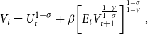(1) \begin{equation} V_{t}=U_{t}^{1-\sigma }+\beta \!\left [ E_{t}V_{t+1}^{\frac{1-\gamma }{1-\sigma }}\right ] ^{\frac{1-\sigma }{1-\gamma }}, \end{equation}

with respect to its flow budget constraint (derived below). $\beta \in (0,1)$ is the subjective discount factor. Utility ( $U$ ) at period $t$ is derived from consumption ( $C_{t}$ ) and leisure ( $1-L_{t}$ ) and is of the non-separable form proposed by Greenwood et al. (Reference Greenwood, Hercowitz and Huffmann1988):

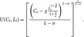(2) \begin{equation} U(C_{t},L_{t})=\left [ \frac{\left ( C_{t}-\chi \frac{L_{t}^{1+\frac{1}{\varphi }}}{1+\frac{1}{\varphi }}\right ) ^{1-\sigma }}{1-\sigma }\right ] ^{\frac{1}{1-\sigma }}. \end{equation}

In the expression (2), $\sigma$ is related to the inverse of the intertemporal elasticity of substitution (IES) as $\sigma ^{-1}/(1+\varphi )$ , where $\varphi$ is the Frisch elasticity of labor supply to wages. $\chi \gt0$ pins down hours worked in steady state. The connection between the coefficient of relative risk aversion ( $CRRA$ ) and parameter $\gamma$ of the recursive utility in equation (1) is given by [for steps of the derivations see Swanson (Reference Swanson2012)]:

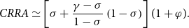\begin{equation*} \textit{CRRA}\simeq \left [ \sigma +\frac {\gamma -\sigma }{1-\sigma }\left ( 1-\sigma \right ) \right ] (1+\varphi ). \end{equation*}

The previous expression tells us that CRRA increases with Frisch elasticity. With GHH utility, the wealth effect of the technology shock on labor supply is eliminated, and labor input becomes persistently procyclical. Unlike separable preferences, labor does not have insurance property in the case of bad shocks.Footnote ⁷ Hence, more flexible labor supply ( $\varphi$ higher) implies more risks (asset returns more procyclical) and households show higher aversion to risks (CRRA is higher). As a result, the propagation of the technology shock is stronger: consumption and dividends exhibit higher comovement and carry higher a price of risk.

Households possess two types of assets: shares in a mutual fund of firms and government bonds. Let $x_{t}$ denote the share in the mutual fund of firms entering period $t$ . In each period, the mutual fund pays the representative household the total profit (in units of currency) of all firms that produce in that period, $P_{t}N_{t}d_{t}$ . In period $t$ , the representative household purchases $x_{t+1}$ shares in a mutual fund of $N_{H,t}\equiv N_{t}+N_{E,t}$ firms where the first term refer to firms already operating at time $t$ while the second term stands for the new entrants. Only $N_{t+1}=(1-\delta )N_{H,t}$ firms will produce and pay dividends at time $t+1$ . As the household has no information about which $\delta$ share of firms are induced to leave the market at the end of period $t$ , it finances the continuing operation of all preexisting firms and all new entrants during period $t$ .

The nominal price of a claim to the future profit stream of the mutual fund of $N_{H,t}$ firms at time $t$ equals to $S_{t}^{\text{ex,nom}}\equiv P_{t}S_{t}^{ex}$ where the superscript $\text{ex,nom}$ marks the ex-dividend price in nominal terms. At time $t$ , the representative household holds nominal bonds and a share $x_{t}$ in the mutual fund. It receives labor income, $W_{t}L_{t}$ , interest income $i_{t-1}$ on nominal bonds. The share in the mutual fund brings dividend income (in nominal terms), $D_{t}^{\text{nom}}\equiv P_{t}d_{t}$ , plus the current nominal value of selling the shares, $S_{t}^{\text{ex,nom}}$ . Therefore, the period budget constraint of the representative household (in units of currency) can be written as:

\begin{equation*} B_{N,t+1}+S_{t}^{\text{ex,nom}}N_{H,t}x_{t+1}+P_{t}C_{t}=(1+i_{t-1})B_{N,t}+(D_{t}^{\text{nom}}+S_{t}^{\text{ex,nom}})N_{t}x_{t}+W_{t}L_{t}+T_{t}^{L}\end{equation*}

where $D_{t}^{\text{nom}}$ stands for the nominal value of dividends, $D_{t}^{\text{nom}}\equiv P_{t}d_{t}$ , $1+i_{t}$ is the gross nominal interest rate, and $T_{t}^{L}$ are lump-sum taxes in nominal terms.

Based on the Dixit-Stiglitz functional form for the consumption bundle and price aggregators, the connection between relative prices and the number of firms (varieties) in the symmetric equilibrium is given by:

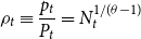(3) \begin{equation} \rho _{t}\equiv \frac{p_{t}}{P_{t}}=N_{t}^{1/(\theta -1)} \end{equation}

where $1/(\theta -1)$ is net markup. The consumer price index ( $P_{t}$ ) differs from the producer price index ( $p_{t}$ ) as the former does not include the effect of rising varieties captured $N_{t}^{1/(\theta -1)}$ .

Let PPI and CPI inflation rates be denoted, respectively, by

\begin{align*} \Pi _{t} & =1+\pi _{t}=\frac{p_{t}}{p_{t-1}}\\ \Pi _{t}^{C} & =1+\pi _{t}^{C}=\frac{P_{t}}{P_{t-1}} \end{align*}

where $\pi _{t}$ and $\pi _{t}^{C}$ are the net while $\Pi _{t}$ and $\Pi _{t}^{C}$ are the gross PPI and CPI inflation rates, respectively. Hence, the connection between PPI and CPI inflation comes from the variety effect:

(4) \begin{equation} \frac{\Pi _{t}}{\Pi _{t}^{C}}=\left ( \frac{N_{t}}{N_{t-1}}\right ) ^{1/(\theta -1)}. \end{equation}

Next, we list the optimality conditions of the households.

The intratemporal condition is given by:

(5) \begin{equation} w_{t}=\chi L_{t}^{1/\varphi }. \end{equation}

The bond Euler equation:

\begin{equation*} 1=E_{t}\!\left ( M_{t,t+1}\frac {1+i_{t}}{\Pi _{t+1}^{C}}\right ), \end{equation*}

where the stochastic discount factor is given by:

(6) \begin{equation} M_{t,t+1}=\beta \frac{\text{MUC}_{t+1}}{\text{MUC}_{t}}\left ( \frac{V_{t+1}^{1/(1-\sigma )}}{\tilde{V}_{t}^{1/(1-\gamma )}}\right ) ^{\sigma -\gamma }\text{where }\tilde{V}_{t}\equiv E_{t}V_{t+1}^{\frac{1-\gamma }{1-\sigma }}\text{.} \end{equation}

Based on the function form in expression (2), the marginal utility of consumption is given by

(7) \begin{equation} \text{MUC}_{t}\equiv \left ( C_{t}-\chi \frac{L_{t}^{1+\frac{1}{\varphi }}}{1+\frac{1}{\varphi }}\right ) ^{-\sigma }. \end{equation}

The share Euler equation can be written as:

\begin{equation*} 1=(1-\delta )E_{t}\!\left ( M_{t,t+1}\frac {S_{t+1}^{\text{ex}}+d_{t+1}}{S_{t}^{\text{ex}}}\right ), \end{equation*}

where $S_{t}^{\text{ex}}\equiv S_{t}^{\text{ex,nom}}/P_{t}$ is the real ex-dividend share price and firm-level dividends, $d_{t}$ , follow:

\begin{equation*} d_{t}=\left ( 1-\frac {1}{\mu _{t}}-\frac {\phi _{P}}{2}\pi _{t}^{2}\right ) \frac {Y_{t}}{N_{t}}. \end{equation*}

2.2. The firms’ problem

There are two types of firms. Final good firms bundle goods produced by intermediaries. The cost-minimization problem of the final good firms leads to the total demand schedule for product $\omega$ :

(8) \begin{equation} y_{t}(\omega )=\left ( \frac{p_{t}(\omega )}{P_{t}}\right ) ^{-\theta }(C_{t}+\text{PAC}_{t}), \end{equation}

where $\text{PAC}_{t}=N_{t}\text{pac}_{t}$ denotes the nominal value of aggregate price adjustment costs [firm-level price adjustment costs are defined in equation (10)]. Intermediaries take the demand schedule in equation (8) as given when maximizing their profits.

There is a mass of intermediary firms. Firm $\omega$ employs labor, $l_{t}(\omega )$ , in order to produce output, $y_{t}(\omega )$ , using a constant-return-to-scale technology: $y_{t}(\omega )=Z_{t}l_{t}(\omega )$ where $Z_{t}$ is a stationary productivity shock:

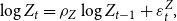\begin{equation*} \log Z_{t}=\rho _{Z}\log Z_{t-1}+\varepsilon _{t}^{Z}\text {,}\end{equation*}

where $\varepsilon _{t}^{Z}$ is an independently and identically distributed (iid) stochastic technology disturbance with mean zero and variance $\sigma _{Z}^{2}$ . The unit cost of production is the real marginal cost which is given by $w_{t}/Z_{t}$ where $w_{t}\equiv W_{t}/P_{t}$ is the real wage.

There is also a mass of prospective entrants. Firms pay an entry cost of $f_{E}$ in consumption units. Each period $\delta$ fraction of firms exit. New entrants ( $N_{E}$ ) and incumbents survive with probability $1-\delta$ . The model features a time-to-build lag in the sense that firms entering at time $t$ start to produce one period later. Therefore, the number of active firms at period $t$ , $N_{t}$ , is described by:

(9) \begin{equation} N_{t}=(1-\delta )(N_{t-1}+N_{E,t-1}). \end{equation}

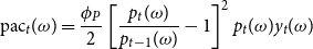
Adjusting prices is costly for intermediary goods-producing firms. Hence, nominal rigidity is introduced in the form of price adjustment costs that can be described with a quadratic function as in Rotemberg (Reference Rotemberg1982):

(10) \begin{equation} \text{pac}_{t}(\omega )=\frac{\phi _{P}}{2}\left [ \frac{p_{t}(\omega )}{p_{t-1}(\omega )}-1\right ] ^{2}p_{t}(\omega )y_{t}(\omega ) \end{equation}

where $\phi _{P}$ governs the strength of price adjustment costs. The real profits of firm $\omega$ at time $t$ (transferred back to households in the form of dividends) are given by:

(11) \begin{equation} d_{t}(\omega )=\frac{p_{t}(\omega )}{P_{t}}y_{t}(\omega )-w_{t}l_{t}(\omega )-\frac{\text{pac}_{t}(\omega )}{P_{t}}. \end{equation}

Firms face a death shock occurring with probability $\delta \in (0,1)$ in each period. In each period, firm $\omega$ continues with probability $1-\delta$ and maximizes profits by choosing $p_{t}(\omega )$ optimally:

(12) \begin{equation} \underset{p_{t}(\omega )}{\max }E_{0}\left \{{\displaystyle \sum \limits _{t=0}^{\infty }} [\beta (1-\delta )]^{t}M_{t,t+1}d_{t}(\omega )\right \}, \end{equation}

with respect to equations (3), (11), and (8). Optimal choice of the firm leads to the pricing condition:

\begin{equation*} \frac {p_{t}(\omega )}{P_{t}}=\mu _{t}\frac {w_{t}}{Z_{t}}\end{equation*}

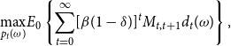
where $\mu _{t}$ denotes the gross markup function which is time-varying due to sticky prices:

\begin{align*} \mu _{t} & \equiv \frac{\theta }{(\theta -1)\left ( 1-\frac{\phi _{P}}{2}\pi _{t}^{2}\right ) +\phi _{P}\pi _{t}(1+\pi _{t})-\beta E_{t}\!\left \{ \Upsilon _{t+1}\right \} }\\ \text{with }\Upsilon _{t+1} & \equiv (1-\delta )M_{t,t+1}\phi _{P}\pi _{t+1}\frac{Y_{t+1}}{Y_{t}}\frac{N_{t}}{N_{t+1}}\left ( 1+\pi _{t+1}\right ) \end{align*}

where $\pi _{t}\equiv \log\! (p_{t}/p_{t-1})=\log\! (\Pi _{t})$ . In the zero inflation steady state ( $\pi =0$ ), the gross markup is given by $\mu \equiv \theta/(\theta -1)$ . $M_{t,t+1}$ is the stochastic discount factor defined in equation (6).

The value of the firm is linked to the entry cost (free entry condition) as:

\begin{equation*} S_{t}^{\text{ex}}=f_{E}. \end{equation*}

The free entry condition helps to pin down the number of firms in equilibrium.

2.3. Monetary policy

Monetary policy is described by a simple Taylor rule of the form:

(13) \begin{equation} R_{t}=\frac{1}{\beta }R_{t-1}^{\rho }\left [ (\Pi _{t})^{\phi _{\pi }}\left ( Y_{t}^{R}/Y_{t-1}^{R}\right ) ^{\phi _{Y}}\right ] ^{1-\rho }, \end{equation}

where $R_{t}\equiv 1+i_{t}$ is the gross nominal interest rate and inflation is zero in the steady state. Coibion and Gorodnichenko (Reference Coibion and Gorodnichenko2011) as well as Sims (Reference Sims2013) mention two reasons why it is better to include output growth in the Taylor rule instead of measures of the output gap: (i) output growth is observable in real time to policymakers while output gap estimates display great variety and (ii) output growth targeting induces welfare gains relative to output gap targeting. Hence, our robustness check with a Taylor rule includes output growth as a measure of the output gap.

2.4. Equilibrium

In the symmetric equilibrium, all firms make identical choices so that $p_{t}(\omega )=p_{t}$ , $d_{t}(\omega )=d_{t}$ , $y_{t}(\omega )=y_{t}$ , $S_{t}^{\text{ex}}(\omega )=S_{t}^{\text{ex}}$ , $l_{t}(\omega )=l_{t}$ , $\mu _{t}(\omega )=\mu$ , and $\text{pac}_{t}(\omega )=\text{pac}_{t}$ . Net bond holdings are zero $B_{t}=B_{t+1}=0$ and $x_{t}=x_{t+1}=1$ .

The labor market clearing is given by:

(14) \begin{equation} L_{t}=N_{t}l_{t}. \end{equation}

The aggregate production function can be derived as:

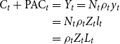\begin{align*} C_{t}+\text{PAC}_{t} & =Y_{t}=N_{t}\rho _{t}y_{t}\\ & =N_{t}\rho _{t}Z_{t}l_{t}\\ & =\rho _{t}Z_{t}L_{t} \end{align*}

The last row contains the aggregate production function, and the term $\rho _{t}$ can be interpreted as an endogenous component of productivity. The full list of equilibrium conditions can be found in the online appendix.

2.5. Asset prices

In this subsection, we show how we price claims on various cash flows such as consumption, output, dividends, and labor income.

The real cum-dividend price, $S_{t}^{\mathcal{Q}}$ , of a cash flow $\{\mathcal{Q}_{t+s}\}_{s=0}^{\infty }$ is given by

\begin{equation*} S_{t}^{\mathcal {Q}}\equiv E_{t}\!\left [{ \sum \limits _{s=1}^{\infty }} M_{t,t+s}\mathcal {Q}_{t+s}\right ] \end{equation*}

Note that we price a claim on consumption ( $\mathcal{Q}_{t}=C_{t}$ ), labor income ( $\mathcal{Q}_{t}=\text{LI}_{t}=\frac{W_{t}}{P_{t}}L_{t}$ ), etc. The stochastic discount factor is model-specific and is used to price the cash flow of various claims.

The previous expression can alternatively be written recursively as:

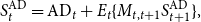\begin{equation*} S_{t}^{\text{AD}}=\text{AD}_{t}+E_{t}\{M_{t,t+1}S_{t+1}^{\text{AD}}\}, \end{equation*}

where $\mathcal{Q}_{t}=\text{AD}_{t}=N_{t}d_{t}$ , and $S_{t}^{\text{AD}}$ is the cum-dividend price of the aggregate dividend claim.

The previous expression can be written in Euler equation form as:

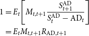\begin{align*} 1 & =E_{t}\!\left [ M_{t,t+1}\frac{S_{t+1}^{\text{AD}}}{S_{t}^{\text{AD}}-\text{AD}_{t}}\right ] \\ & =E_{t}M_{t,t+1}R_{\text{AD},t+1} \end{align*}

where the return on the AD claim is given by:

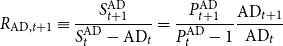(15) \begin{equation} R_{\text{AD},t+1}\equiv \frac{S_{t+1}^{\text{AD}}}{S_{t}^{\text{AD}}-\text{AD}_{t}}=\frac{P_{t+1}^{\text{AD}}}{P_{t}^{\text{AD}}-1}\frac{\text{AD}_{t+1}}{\text{AD}_{t}} \end{equation}

where $P_{t}^{\text{AD}}\equiv S_{t}^{\text{AD}}/\text{AD}_{t}$ is the price-dividend ratio. Our measure of equity risk premium is the levered excess return based on aggregate dividends:

\begin{equation*} \text{EQPR}_{t}=\phi _{{lev}}(\ln R_{\text{AD},t}-\ln R_{f,t-1}), \end{equation*}

where the excess return is leveraged (see the leverage factor $\phi _{{lev}}$ ) as in Croce (Reference Croce2014). Aggregate dividends are linked to aggregate output and, hence, follow its procyclical pattern.

2.6. The adjusted wealth portfolio

We follow Li and Palomino (Reference Li and Palomino2014) and use the so-called return representation of the pricing kernel to identify its short- and long-run components. The return representation includes the return on the adjusted wealth portfolio in the pricing kernel instead of the continuation value of utility which is difficult to interpret. In particular, the cash flow of the adjusted wealth portfolio (containing the consumption and labor income claims) is linked to current and future consumption and labor income streams.

Let $Q_{t}$ denote cash flow for the claim on the adjusted wealth portfolio:

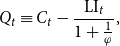(16) \begin{equation} Q_{t}\equiv C_{t}-\frac{\text{LI}_{t}}{1+\frac{1}{\varphi }}, \end{equation}

where $\text{LI}_{t}=\frac{W_{t}}{P_{t}}L_{t}$ . The SDF in equation (6) can be written in its return form as (for steps of the derivations see the online appendix of LP):

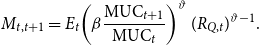(17) \begin{equation} M_{t,t+1}=E_{t}\!\left ( \beta \frac{\text{MUC}_{t+1}}{\text{MUC}_{t}}\right ) ^{\vartheta }(R_{Q,t})^{\vartheta -1}. \end{equation}

where $\vartheta \equiv \frac{1-\gamma }{1-\sigma }$ . We take the natural log of equation (17) and identify the short- and long-run components as in Li and Palomino (Reference Li and Palomino2014):

(18) \begin{equation} m_{t,t+1}=\vartheta \ln \beta +E_{t}m_{t,t+1}^{\text{SR}}+E_{t}m_{t,t+1}^{\text{LR}} \end{equation}

where

(19) \begin{align} m_{t,t+1}^{\text{SR}} &\equiv -\vartheta \Delta \text{muc}_{t+1}-(1-\vartheta )\Delta q_{t+1} \end{align}

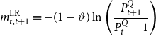(20) \begin{align} m_{t,t+1}^{\text{LR}} &\equiv -(1-\vartheta )\ln \left ( \frac{P_{t+1}^{Q}}{P_{t}^{Q}-1}\right )\end{align}

where $\Delta \text{muc}_{t+1}=\ln\! (\Delta \text{MUC}_{t+1})$ , $\Delta q_{t+1}=\ln\! (\Delta Q_{t+1})$ , and $\ R_{Q,t}$ is decomposed into the log of price-cash flow ratio and the log of the growth rate of $Q$ [similar to equation (15)]. Hence, the short-run component, $m_{t,t+1}^{\text{SR}}$ contains the log of consumption and labor income growth while the long-run component is related to the log of price-cash flow ratio on the adjusted wealth portfolio.

The price-cash-flow ratio and the return on the $Q$ claim is, however, related to the discounted future utility from future consumption and labor income streams. In the entry model, bad shocks to current consumption and labor income are also bad news for future consumption and labor income implying long-run risks. Hence, the short- and long-term components comove positively with firm entry resulting in more volatile pricing kernel and a higher price of risk on the consumption and labor income claims.

2.7. Closed-form illustration

To understand determinants of the excess return on the adjusted wealth portfolio, we assume that $M_{t,t+1}$ and $R_{Q,t+1}$ are jointly conditionally lognormally distributed and derive an analytical expression for the excess return on claim $Q$ as follows (for similar derivations see LPFootnote ⁸ ):

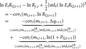(21) \begin{align} & \ln E_{t}R_{Q,t+1}-\ln R_{f,t}+\frac{1}{2}[\text{std}_{t}(\ln E_{t}R_{Q,t+1})]^{2}\nonumber \\ &\quad =-\text{cov}_{t}(m_{t,t+1},\ln R_{Q,t+1})\nonumber \\ & \quad=\underset{\simeq \text{corr}_{t}(m_{t,t+1},m_{t+1}^{\text{SR}})\text{std}_{t}(m_{t,t+1})\text{std}_{t}(m_{t,t+1}^{\text{SR}})}{\underbrace{-\text{cov}_{t}(m_{t,t+1},\Delta q_{t+1})}}\\ &\qquad+ \underset{\simeq \text{corr}_{t}(m_{t,t+1},m_{t+1}^{\text{LR}})\text{std}_{t}(m_{t,t+1})\text{std}_{t}(m_{t,t+1}^{\text{LR}})}{\underbrace{-\text{cov}_{t}(m_{t,t+1},\ln\! (1+P_{Q,t+1}))}}\nonumber \end{align}

where $R_{f,t}$ is the one-period gross real risk-free rate satisfying $1/R_{f,t}=E_{t}M_{t,t+1}$ , $m_{t,t+1}=\ln M_{t,t+1}$ and $q_{t}=\ln\! (Q_{t})$ . In the first row of equation (21), $\frac{1}{2}[\text{std}_{t}(\ln E_{t}R_{Q,t+1})]^{2}$ is the usual Jensen’s inequality term that pops up in lognormal approximations. The last row of equation (21) decomposes the covariances into correlations and standard deviations as well as makes use of expressions (19) and (20). As long as the correlation between $m$ and $m^{\text{LR}}$ (or, equivalently, the correlation between $m^{\text{SR}}$ and $m^{\text{LR}}$ as $m=m^{\text{SR}}+m^{\text{LR}}$ ) is positive, the excess return has a component that compensates for long-run risks. Below we show that the long-run component positively comoves with the short-run component and the whole pricing kernel in two ways: (i) by presenting impulse responses and (ii) unconditional correlations of $m^{\text{LR}}$ with $m^{\text{SR}}$ and $m$ as well as standard deviations.

4.1. Impulse responses from the benchmark model

To explain the mechanisms in the entry model, we consider impulse responses and simulated model moments compared to the data. Model moments are based on simulations for 10,000 quarters using second-order perturbation. We start with the impulse responses. In particular, we consider a positive one-standard deviation productivity shock which induces the entry of new firms due to positive profit opportunities. The impact of positive technology shock to macro- and finance variables is shown on Figures 2 and 3, respectively.

Figure 2 shows that a positive technology shock triggers firm entry leading to the growth in the log of the number of firms ( $n$ ) and a rise in the log of relative prices ( $\rho$ ).Footnote ¹⁰ The positive wealth effect of the productivity boosts consumption ( $c$ ), output ( $y$ ), and labor ( $l$ ) as well with similar rising pattern over time. Figure 3 presents that the log of labor income ( $li$ ) and aggregate dividends ( $ad$ ) both expand after a positive technology shock. Investors require higher return on consumption and labor income claims as well as the adjusted wealth portfolio (see variables $r_{C}$ , $r_{\text{LI}}$ , and $r_{Q}$ , respectively, on Figure 3) also react more in the entry model. Further, the persistent rise in expected consumption, labor income, and aggregate dividends implies long-run risks. The graphs are displayed for the cases of IES $\gt$ 1 (our benchmark) and IES $\lt$ 1. IES $\gt$ 1 implies that the substitutability between current and future consumption is high, and there is complementarity between current utility and the continuation value of utility. An IES $\lt$ 1 leads to consumption smoothing.

Consistent with the results in Tables 2 and 3 (see the subsection “long-run risks” below), Figure 1 shows that the entry model enhances the propagation of technology shocks. In particular, the variables in the entry model display greater and more persistent response to TFP shocks relative to the no-entry model. The persistent variation in the entry model survives in the case of separable preferences too, see Figures 4 and 5.

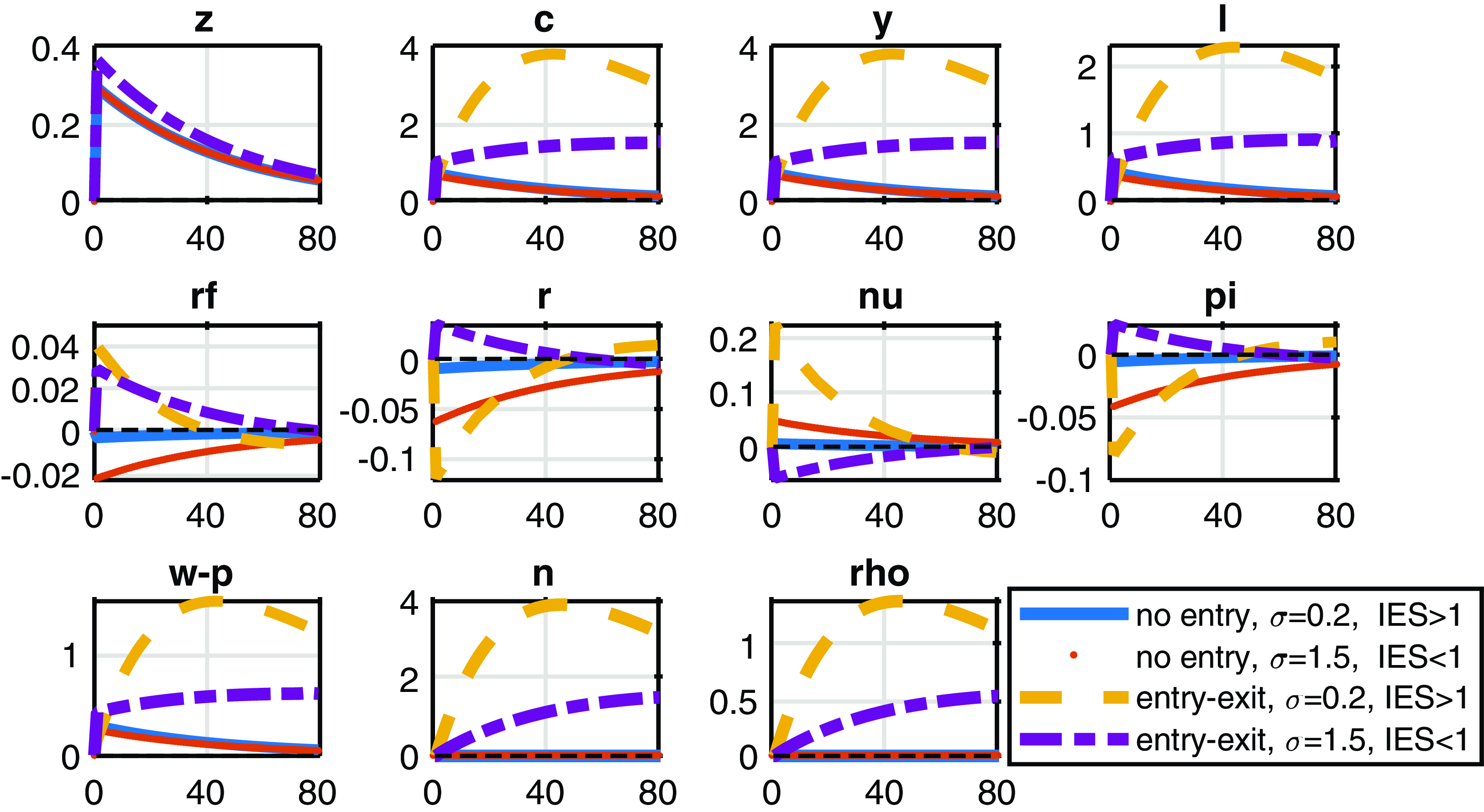
Figure 2. The response of macroeconomic variables to a positive technology shock. Notes: the responses from the no-entry (solid) and entry (dashed) models are displayed. Vertical axes measure percentage deviation of the variables from the steady state. The log deviation of nominal and risk-free real interest rates ( $r$ and $r_{f}$ ) and the inflation ( $\pi$ ) are annualized. For instance, $z$ is the log of temporary exogenous technology in percentage deviation from the steady state: $z_{t}=100\ln(Z_{t}/Z)$ . The rest of the variables are consumption, $c$ , output, $y$ , labor, $l$ , the markup, $\mu$ , real wage, $w-p$ , number of firms, $n$ , variety effect, and $rho$ .

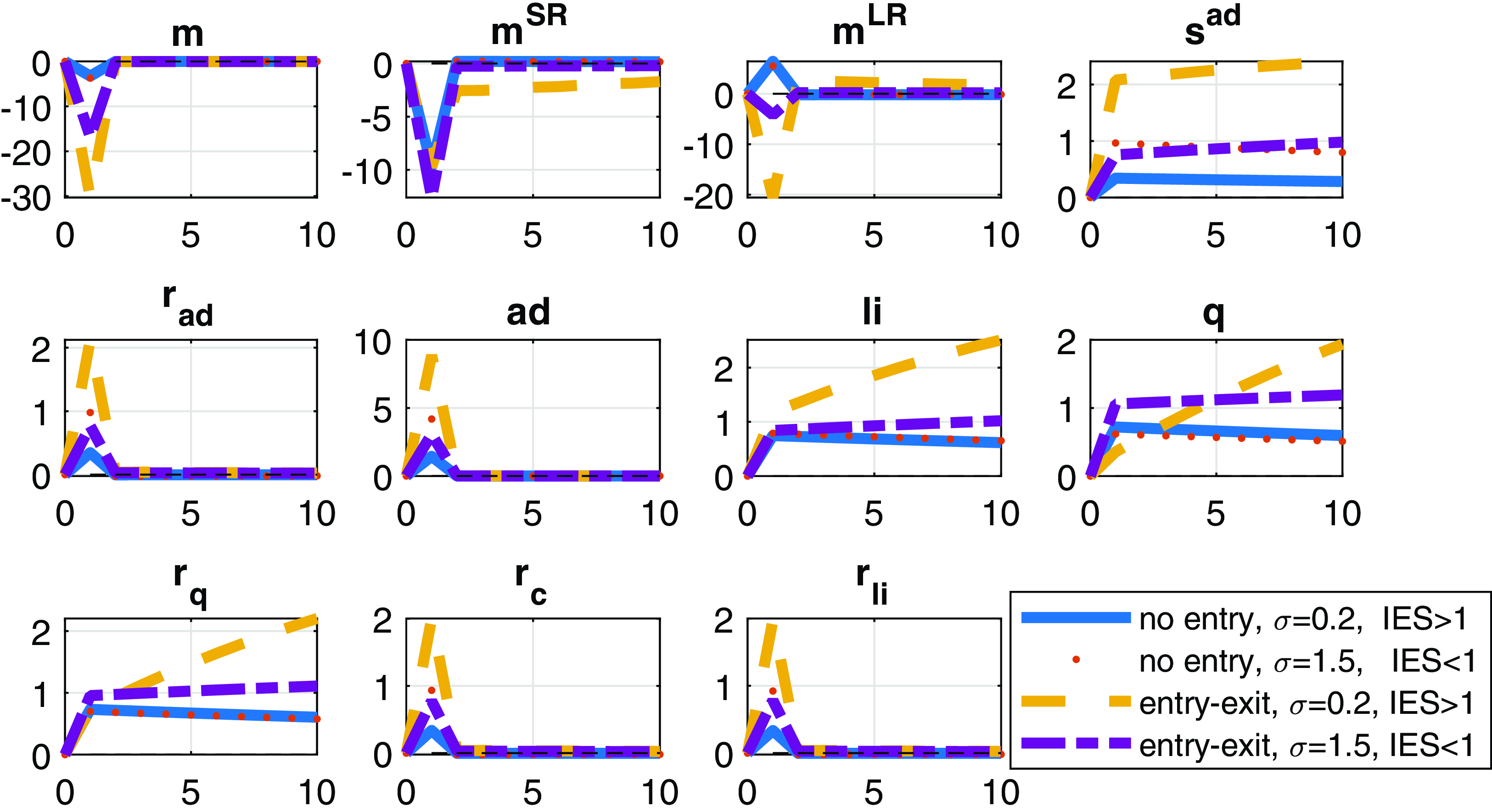
Figure 3. The response of financial variables to a positive technology shock. Notes: the responses from the no-entry (solid) and entry (dashed) models are displayed. Vertical axes measure percentage deviation of the variables from the steady state. Log-returns ( $r_{q}$ , $r_{c}$ , $r_{\text{li}}$ , and $r_{\text{ad}}$ ) are annualized. The following list of variables is displayed. $m$ is real the pricing kernel with short-run, $m^{\text{SR}}$ and long-run components, $m^{\text{LR}}$ . The price of the aggregate dividend claim, $s^{\text{ad}}$ , the payoff on the composite claim, $q$ , aggregate dividends, ad, return on aggregate dividend claim, $r_{\text{ad}}$ , return on the consumption claim, $r_{c}$ , labor income, $\text{li}$ , and return on the labor income claim, $r_{\text{li}}$ .

It is of interest to compare our results to Li and Palomino (Reference Li and Palomino2014) who used separable preferences, several types of shocks (transitory technology, permanent technology, and monetary policy shocks) as well as price and wage rigidity. They plot growth rates in response to each of their shocks. To make the comparison in a transparent way, we display variables of our model with separable preferences as growth rates on Figure 6. Our impulse responses are made for the case of flexible prices (no price rigidity) so that they reflect the effect of firm entry only. Inspecting the plots of LP (see, e.g. Figure 2 in their online appendix), there is virtually no persistence in their growth rates even with permanent shocks: the main variables of interest such as consumption growth return to the steady state even after one period (in their baseline scenario as well as in the case of either price or wage rigidity). However, consumption growth in the entry model exhibits persistence even in response to transitory technology shocks in the absence of price rigidity.

Next, we explain how long-run risk emerges in the entry model.

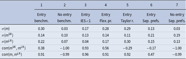
Table 2. The decomposition of the pricing kernel

Notes: This table contains unconditional correlations and standard deviations from the log of the pricing kernel ( $m$ ) which is decomposed into short- and long-run parts (see $m^{\text{SR}}$ and $m^{\text{LR}}$ , respectively ) in the spirit of Li and Palomino (Reference Li and Palomino2014). The abbreviation benchm. refers to the benchmark parametrization. Flex. pr. refers to the case of flexible prices. Taylor refers to a Taylor-type interest rate rule with the inclusion of a response to the output gap and having interest rate smoothing. Columns 1–5 are generated by GHH preferences while columns 6 and 7 use separable preferences.

Table 3. Finance moments and properties of consumption growth

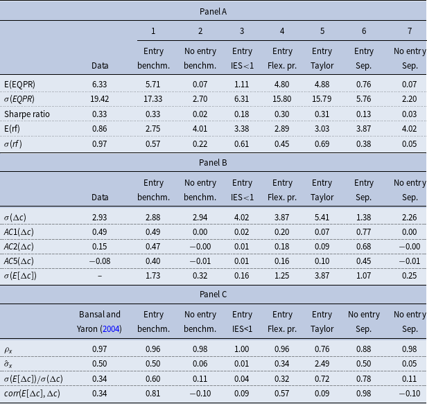
Notes: notations are identical to Table 2. In the rows, E(.), $\sigma (.)$ , and corr(.,.) refer to unconditional mean, standard deviation, and correlations, respectively. AC1, 2, and 5 refer to first-, second-, and .fifth-order autocorrelations, respectively. Panel A contains financial moments. Panel B contains statistics related to consumption growth. In Panel C, we fit the expected consumption growth, $E[\Delta (c)]$ from the entry and no-entry models to an AR(1) process $x_t=\rho _{x} x_{t-1}+\sigma _{x} \epsilon _{x,t}$ , where $\epsilon _{x,t} \sim N(0,1)$ , and compare to the exogenous consumption growth process in Bansal and Yaron (Reference Bansal and Yaron2004). We report the persistence parameter and the annualized volatility parameter, $\tilde{\sigma }_{x}$ , from the fitted AR(1) process.

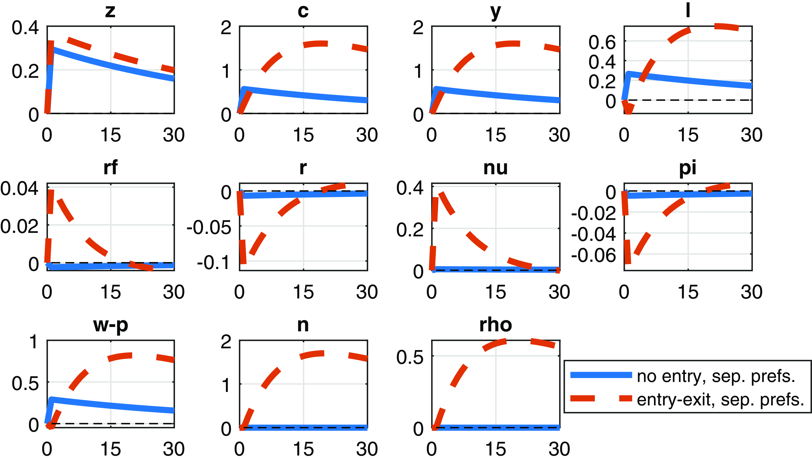
Figure 4. Impulse responses of selected variables to a positive technology shock. Separable preferences of the form $\frac{C^{1-\sigma }}{1-\sigma }-\chi \frac{L^{1+\frac{1}{\varphi }}}{1+\frac{1}{\varphi }}$ are considered.

Figure 5. Impulse responses of selected variables to a positive technology shock. Separable preferences of the form $\frac{C^{1-\sigma }}{1-\sigma }-\chi \frac{L^{1+\frac{1}{\varphi }}}{1+\frac{1}{\varphi }}$ are considered.

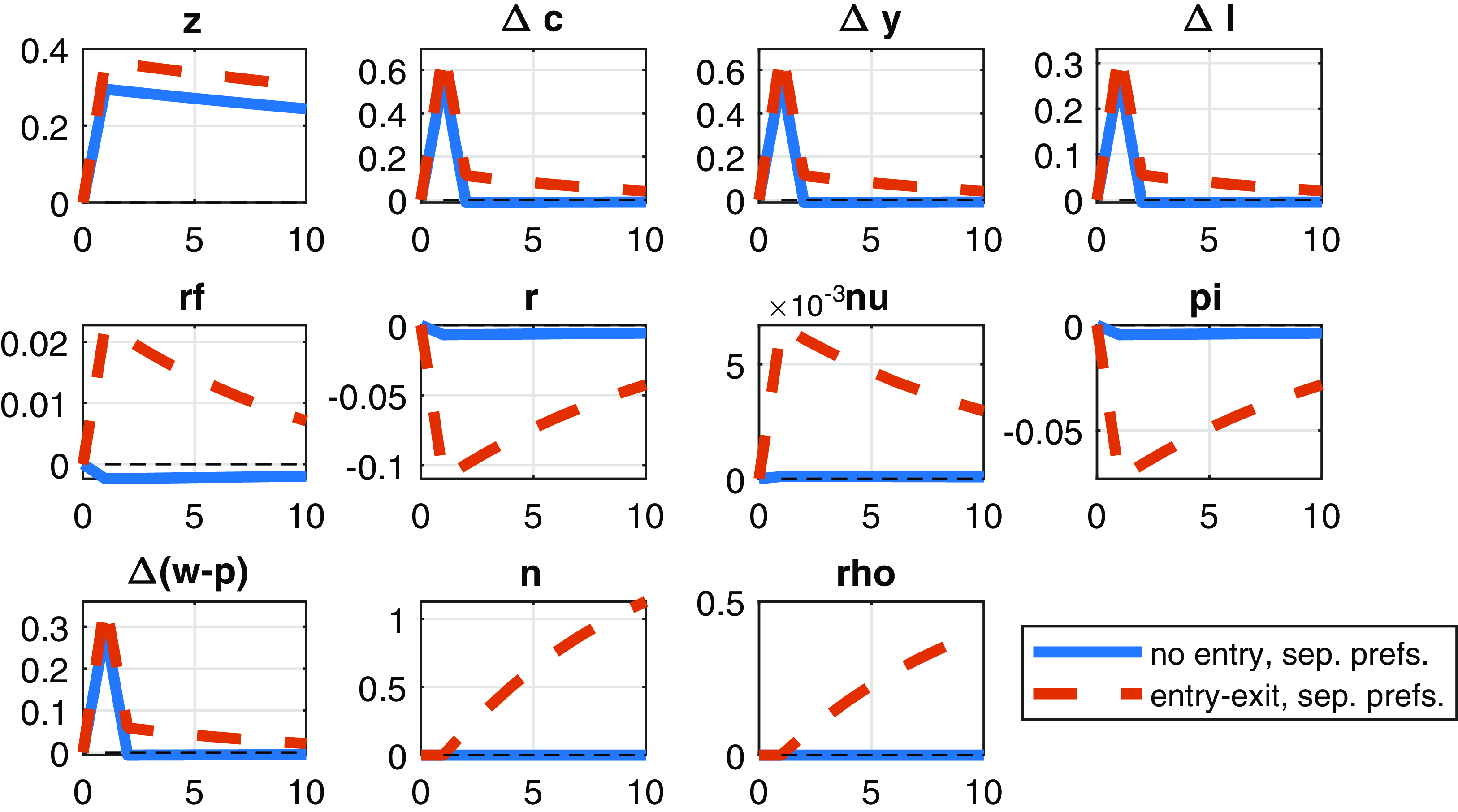
Figure 6. Impulse responses of selected variables to a positive technology shock. Separable preferences of the form $\frac{C^{1-\sigma }}{1-\sigma }-\chi \frac{L^{1+\frac{1}{\varphi }}}{1+\frac{1}{\varphi }}$ are considered. Prices are flexible in this case (see the negligible change in the markup $\mu$ , which is constant with flexible prices).

4.2. Long-run risks

We show the response of the log of the pricing kernel ( $m$ ) as well as its short-run and long-run components (see $m^{\text{SR}}$ and $m^{\text{LR}}$ , respectively) to a positive TFP shock on Figure 3. The sign of the $m^{\text{LR}}$ component differs across the entry and no-entry models. The $m^{\text{SR}}$ and $m^{\text{LR}}$ components move in the same direction in the entry model generating excess movement in $m$ as well as the returns. Hence, the long-term component of the excess return in equation (21) is positive only in the entry model. This can be explained as follows.

In endowment, economy models such as Bansal and Yaron (Reference Bansal and Yaron2004) with long-run risks the short- and long-run components are driven by separate shocks. In our production models, technology shocks contribute to both the short- and long-run components. Hence, the stochastic discount factor is not only driven by the volatility of each of the components but their correlation [see equation (21)] is also important to determine the volatility of the pricing kernel ( $m$ ) and the excess return. In the entry model, shocks move the current and expected consumption as well as the short and long components of the $m$ in the same direction leading to long-run risks.

In Table 2, we report the unconditional standard deviations and correlations between short- and long-run components of the pricing kernel as an approximation to the conditional ones in the decomposition above. Simulated moments in column 2 and 3 are produced with the benchmark model using the benchmark parameterization in Table 1. Column 3–5 include robustness checks with respect to the (i) IES (inversely related to $\sigma$ ), (ii) flexible prices, and (iii) a Taylor rule (with response to output gap as well as interest rate smoothing—see the Taylor rule calibration at the bottom of Table 1). Columns 2–5 are based on non-separable preferences of GHH type. Results in columns 6 and 7 are based on separable preferences using the benchmark calibration.

The results in Table 2 confirm findings from the impulse responses: the short- and long-run components comove positively only in the case of the entry model marking the presence of long-run risks. Further, the standard deviations of $m^{\text{SR}}$ , $m^{\text{LR}}$ , and $m$ are all higher with increasing variety relative to the case of fixed variety. Importantly, the no-entry model in column 2 (based on the benchmark non-separable utility) or in column 7 (employing separable preferences) is unable to produce long-run risks (the correlation between the short- and long-term components is negative).

4.3. The fit to financial data and moments of the consumption growth

Table 3 contains selected macro- and finance moments. The first column contains macroeconomic and finance data moments based on US data 1929–1998 from Bansal and Yaron (Reference Bansal and Yaron2004). In this subsection, we mainly focus on comparing simulated data from the benchmark entry and no-entry models in columns 1 and 2. A separate section below focuses on the robustness checks in columns 3–7.

Interest rates, returns, inflation, and consumption growth are all annualized percentages. Consistent with the method in Bilbiie et al. (Reference Bilbiie, Ghironi and Melitz2007), model-based macroeconomic and financial variables are taken logs and transformed such that they do not include the variety effect and, hence, are comparable with data moments, for example $y_{t}\equiv \ln\! (P_{t}Y_{t}/p_{t})=\ln\! (Y_{t}/\rho _{t})$ . The table contains three panels. Panel A and B contain financial and macroeconomic moments, respectively.Footnote ¹¹ Panel C compares statistics from the Bansal and Yaron (Reference Bansal and Yaron2004) model to our models. We start with the discussion of Panel A.

Panel A shows that the entry model generates 90% of the empirical excess return with a volatility closely matching the data, whereas the no-entry model produces zero mean and little variation in the excess return. The unconditional mean of the risk-free rate is somewhat in excess of the data while its standard deviations are lower than data. Importantly, our results are not coupled with excessively high mean and/or standard deviation of the risk-free rates so that our model is not subject to the risk-free rate puzzle.Footnote ¹²

Panel B shows that both the entry and the no-entry models are calibrated such that they reproduce the standard deviation of realized consumption growth ( $\sigma (\Delta c)$ ). Yet, only the entry model produces positive first-order autocorrelation of consumption growth. Hence, consumption growth in the entry model contains a persistent predictable component unlike the no-entry model where consumption growth is i.i.d. and, hence, unpredictable. Delayed firm entry induces low-frequency movements in productivity engineering predictable movements in expected consumption growth. Indeed, there is significant variation in expected consumption growth, $\sigma (E[\Delta c])$ , in the entry model. Whereas the standard deviation of expected consumption growth has little variability in the no-entry model (less than 20 percent of the corresponding value in the entry model). On the downside, we note, however, that the entry model overpredicts the autocorrelations at lags two and five.

Panel CFootnote ¹³ shows the coefficient and the standard error from an AR(1) process fitted to expected consumption growth which is an exogenous process in the endowment model of Bansal and Yaron (Reference Bansal and Yaron2004). While the estimated autoregressive parameters from our models, $\rho _{x}$ , are close to identical to Bansal and Yaron (Reference Bansal and Yaron2004), we find that the estimated standard deviation, $\tilde{\sigma }_{x}$ , is somewhat larger in the entry model than their endowment model. The estimated standard deviation from the no-entry model is close to zero implying that expected consumption growth exhibits zero variation in the no-entry model. We further find that the relative standard deviation and correlation of expected consumption growth are also higher than the ones in Bansal and Yaron.

4.4. Properties of dividend growth, the price-dividend ratio, and variety growth

Table 4 compares data and model moments on dividend growth, price-dividend ratio, and variety growth. Specifically, panel A compares statistics of dividend growth and the price-dividend ratio across the entry and no-entry models to make the following observations. First, the standard deviation of aggregate dividend growth, $\sigma (\Delta (\text{ad}))$ , is about half of what we see in the data. Second, the correlation between aggregate dividend and consumption growth, $\text{corr}(\Delta (\text{ad}),\Delta c)$ , is overestimated by the entry model. Third, the entry model produces a positive autocorrelation in aggregate dividend growth, $\text{AC1}(\Delta (\text{ad}))$ , that is slightly in excess of the data. The latter can still be interpreted as a success as the no-entry model predicts that the autocorrelation of aggregate dividends is zero. Fourth, the standard deviation of the price-dividend ratio, $\sigma (p-d)$ , is also better captured by the entry model but is still half of the data.

Table 4. Properties of dividend growth, the price-dividend ratio, and variety growth

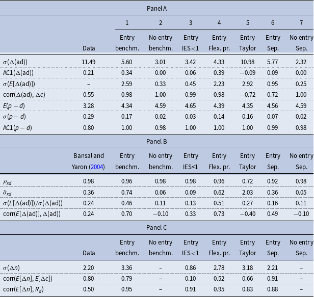
Notes: notations are identical to Table 2. Panel A contains statistics related to aggregate dividend growth and the log of the price-dividend ratio. In Panel B, we fit the expected aggregate dividend growth, $E[\Delta (\text{ad})]$ from the entry and no-entry models to an AR(1) process $xd_t=\rho _{xd} xd_{t-1}+\sigma _{xd} \epsilon _{xd,t}$ , where $\epsilon _{xd,t} \sim N(0,1)$ , and compare to the exogenous dividend growth process in Bansal and Yaron (Reference Bansal and Yaron2004). We report the persistence parameter and the annualized volatility parameter, $\tilde{\sigma }_{xd}$ , from the fitted AR(1) process. Panel C compares moments from the entry model to statistics estimated by Scanlon (Reference Scanlon2019) using US trademark data to proxy variety growth over 1927–2016.

Panel B shows that the entry model has a persistence similar to the exogenous process in Bansal and Yaron ( $\rho _{\text{xd}}$ ) and somewhat higher standard deviation ( $\tilde{\sigma }_{\text{xd}}$ ). Further, we find that the relative standard deviation and correlation between expected and realized dividend growth is overestimated by the entry model to some extent.

Finally, panel C assesses model fit to variety data from Scanlon (Reference Scanlon2019). He proxied the appearance of new products with US trademarks data 1927–2016. In particular, the standard deviation of product growth in the entry model is not distant from the data. Further, the confluence of future product growth and consumption as well as stock returns based on firm-level dividends is also well-captured by the entry model.

4.5. The role of model ingredients

It is of interest to explore whether it is the firm entry mechanism that brings the high equity premium and not other features of our model. In particular, we assess the role of (i) the choice of the elasticity of intertemporal substitution (EIS), (ii) the choice of preferences (separable or non-separable in consumption and hours worked), (iii) price rigidity, and (iv) the form of the Taylor rule. Finally, we highlight why firm entry is more successful in matching financial data relative to LP.

4.5.3. The role of price rigidity and the inclusion of a Taylor rule

With flexible prices, firms operate at their optimal (constant) markups and labor demand is less procyclical. Hence, asset payoffs and returns which are linked to macroeconomic variables through dividends exhibit lower degree of procyclicality, and investors demand lower risk premia. With flexible prices, equity premium drops by about 100 basis points to 480 basis points (see column 4 of Table 3).

Realized consumption growth, however, exhibits higher variation with flexible prices as there is a tighter link between consumption and the technology shock in the absence of markup fluctuations. The volatility of expected consumption growth which is needed for significant long-run risks is lower with flexible prices. The correlation between the short and long parts of the pricing kernel is also lower with flexible prices implying a reduction in long-run risks and risk premia relative to the case of sticky prices.

The specification of interest rate rules has non-negligible impact on equity premia.Footnote ¹⁵ We display impulse responses of model variables to a one-standard deviation technology shock with three different interest rate rules on Figures 7 and 8.

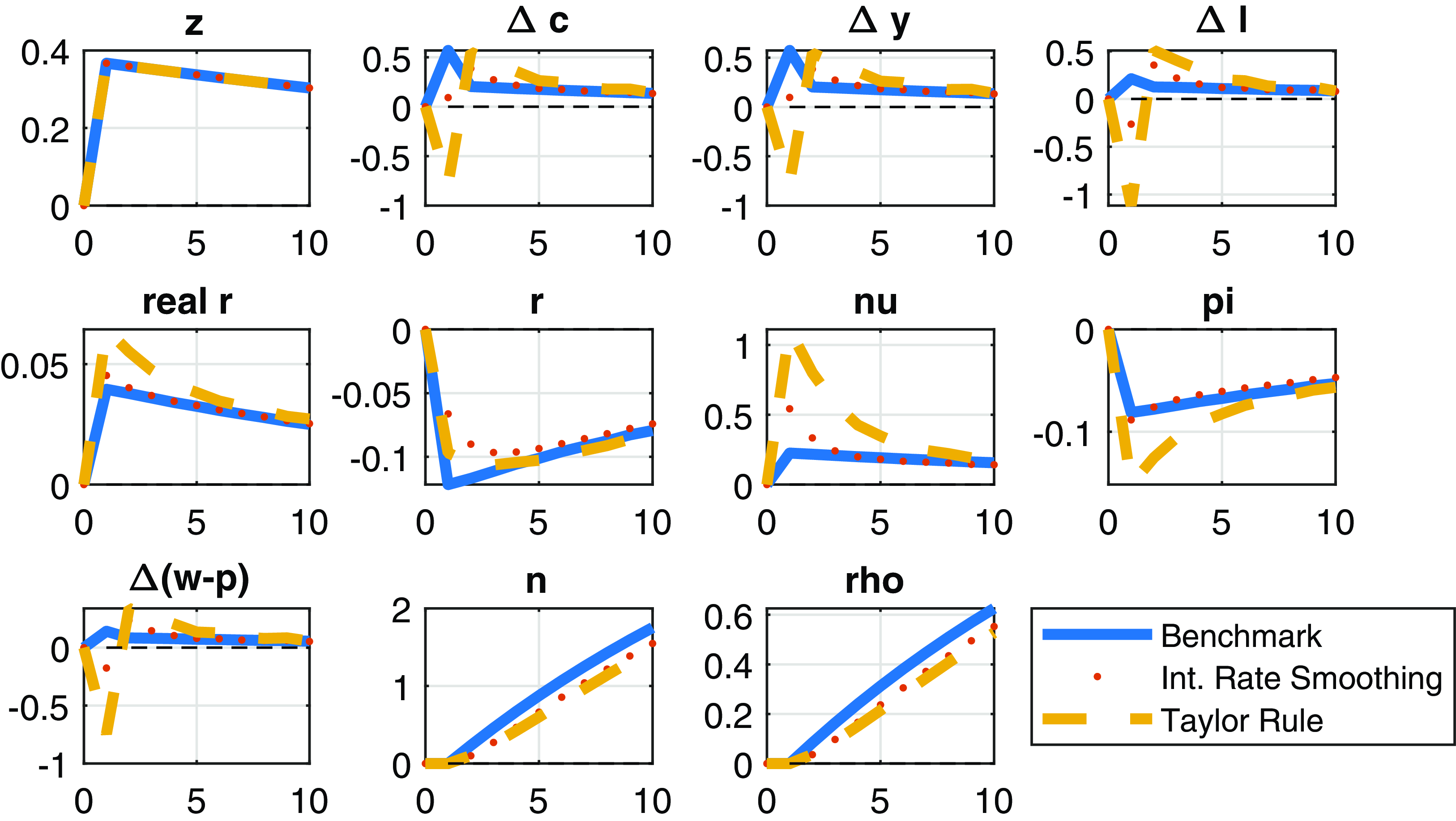
Figure 7. The comparison of three types of interest rate rules in our benchmark model: (i) benchmark rule with response to contemporaneous inflation only (solid); (ii) interest rate rule with smoothing parameter of 0.5 (dotted); (iii) Taylor-type interest rate rule (in line with the calibration in Table 1) with interest rate smoothing as well as response to the output growth (dashed).

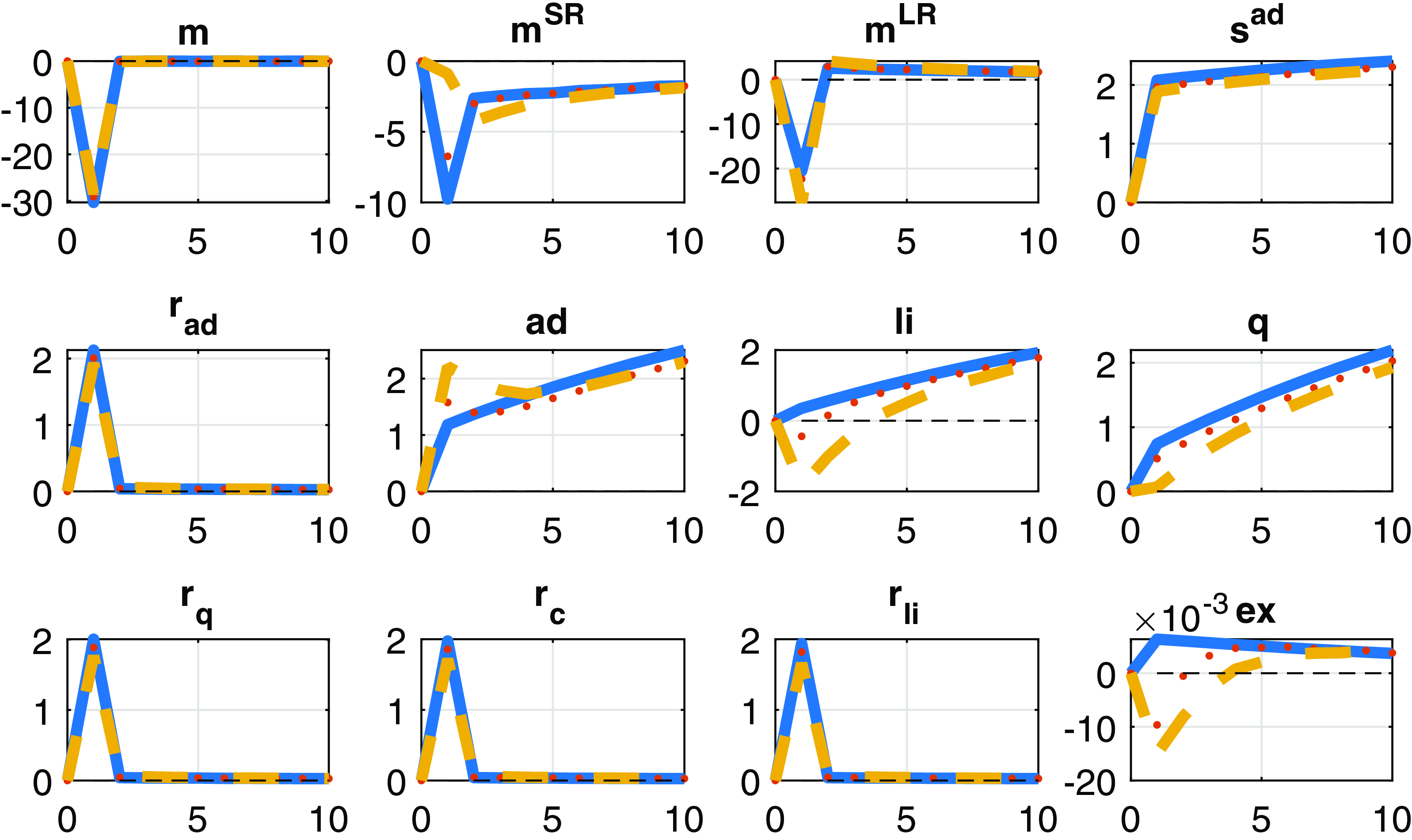
Figure 8. The comparison of three types of interest rate rules in our benchmark model: (i) benchmark rule with response to contemporaneous inflation only (solid); (ii) interest rate rule with smoothing parameter of 0.5 (dotted); (iii) Taylor-type interest rate rule (in line with the calibration in Table 1) with interest rate smoothing as well as response to the output growth (dashed). Ex means the expected excess return on the aggregate dividend claim.

The introduction of interest rate smoothing implies smaller changes in the interest rates and, in equilibrium, less procyclicality and variation in macroeconomic variables reducing the risk premia. The standard deviation of realized consumption growth reduces to 2.44 from 2.88 (benchmark) after the introduction of a small degree of interest smoothing of 0.5 (not reported in the tables). The unconditional mean of the equity premium also reduces to 5.15 from 5.71 (not reported in the tables).

The short-run component of the pricing kernel also displays smaller variation with interest rate smoothing. After a positive shock to technology consumption growth barely moves on impact with interest rate smoothing and leading to lower expected risk premia, $E_{t}[r_{\text{ad},t+1}-r_{f,t}]$ (called “ex” in the bottom right corner of Figure 8) which reduces by −0.014 percentage points on impact.

However, introducing reaction to the output growth by itself raises the standard deviation of variables as well as the risk premia. Taylor-type rules with interest rate smoothing and a reaction to the growth rate of output induce the highest increase in the real interest (called "real r" on the figure) triggering even negative growth rates on impact.

Finally, we consider a Taylor rule with an interest rate smoothing coefficient of 0.7 and a reaction of 0.125 to output growth. Figure 8 shows that the autocorrelation in the short-run component of the pricing kernel changes with a Taylor rule. The latter has the consequence of a negative correlation between the short- and long-run components of the pricing kernel which, by itself, reduces long-run risks and the risk premium. This reduction is, however, mitigated by the rise in the volatility of the expected consumption growth engineering higher standard deviation in the long-run component of the pricing kernel.

Interest rate smoothing dominates the effects of the reaction to the output growth in terms of risk premia: the risk premium decreases by 100 basis points to 488 basis points (see column 5 of Table 3). However, the standard deviation of realized consumption growth is dominated by the reaction to output growth and is more volatile in the Taylor rule scenario.