


1. Introduction
Given a real number $\omega \geqslant 1$ and integers $m,\,r$
 satisfying $0\leqslant r\leqslant m$
 , set
, set

where the binomial coefficient $\binom{m}{i}$ equals $\prod _{k=1}^i\frac {m-k+1}{k}$
 for $i>0$
 and $\binom{m}{0}=1$
 . The weighted binomial sum $g_{\omega,m}(r)$
 and the partial binomial sum $s_m(r)=g_{1,m}(r)$
 appear in many formulas and inequalities, e.g. the cumulative distribution function $2^{-m}s_m(r)$
 of a binomial random variable with $p=q=\tfrac {1}{2}$
 as in remark 5.3, and the Gilbert–Varshamov bound [Reference Ling and Xing6, Theorem 5.2.6] for a code $C\subseteq \{0,\,1\}^n$
 . Partial sums of binomial coefficients are found in probability theory, coding theory, group theory, and elsewhere. As $s_m(r)$
 cannot be computed exactly for most values of $r$
 , it is desirable for certain applications to find simple sharp upper and lower bounds for $s_m(r)$
 . Our interest in bounding $2^{-r}s_m(r)$
 was piqued in [Reference Glasby and Paseman4] by an application to Reed–Muller codes $\textrm{RM}(m,\,r)$
 , which are linear codes of dimension $s_m(r)$
 .
.
Our main result is a generalized continued fraction $a_0 + \mathcal{K}_{i=1}^{r} \frac {b_i}{a_i}$ (using Gauss’ Kettenbruch notation) for $Q:=\frac {(r+1)}{s_m(r)}\binom{m}{r+1}$
 . From this we derive useful approximations to $Q,\, 2+\frac {Q}{r+1}$
 , and $s_m(r)$
 , and with these find a maximizing input $r_0$
 for $g_{\omega,m}(r)$
 .
.
The $j$ th tail of the generalized continued fraction $\mathcal{K}_{i=1}^{r} \frac {b_i}{a_i}$
 is denoted by ${\mathcal {T}}_j$
 where
where

If ${\mathcal {T}}_j=\frac {B_j}{A_j}$ , then ${\mathcal {T}}_j=\frac {b_j}{a_j+{\mathcal {T}}_{j+1}}$
 shows $b_jA_j-a_jB_j={\mathcal {T}}_{j+1}B_j$
 . By convention we set ${\mathcal {T}}_{r+1}=0$
 .
.
It follows from $\binom{m}{r-i}=\binom{m}{r}\prod _{k=1}^i\frac {r-k+1}{m-r+k}$ that $x^i\binom{m}{r}\leqslant \binom{m}{r-i}\le y^i\binom{m}{r}$
 for $0\leqslant i\leqslant r$
 where $x:=\frac {1}{m}$
 and $y:=\frac {r}{m-r+1}$
 . Hence $\frac {1-x^{r+1}}{1-x}\binom{m}{r}\leqslant s_m(r)\leqslant \frac {1-y^{r+1}}{1-y}\binom{m}{r}$
 . These bounds are close if $\frac {r}{m}$
 is near 0. If $\frac {r}{m}$
 is near $\tfrac {1}{2}$
 then better approximations involve the Berry–Esseen inequality [Reference Nagaev and Chebotarev7] to estimate the binomial cumulative distribution function $2^{-m}s_m(r)$
 . The cumulative distribution function $\Phi (x)=\frac {1}{\sqrt {2\pi }}\int _{-\infty }^xe^{-t^2/2}\,dt$
 is used in remark 5.3 to show that $|2^{-m}s_m(r)-\Phi (\frac {2r-m}{\sqrt {m}})|\leqslant \frac {0.4215}{\sqrt {m}}$
 for $0\leqslant r\leqslant m$
 and $m\ne 0$
 . Each binomial $\binom{m}{i}$
 can be estimated using Stirling's approximation as in [Reference Stănică10, p. 2]: $\binom{m}{i}=\frac {C_i^m}{\sqrt {2\pi p(1-p)m}}\left (1+O\left (\frac {1}{m}\right )\right )$
 where $C_i=\frac {1}{p^p(1-p)^{1-p}}$
 and $p=p_i=i/m$
 . However, the sum $\sum _{i=0}^r\binom{m}{i}$
 of binomials is harder to approximate. The preprint [Reference Worsch11] discusses different approximations to $s_m(r)$
 .
.
Sums of binomial coefficients modulo prime powers, where $i$ lies in a congruence class, can be studied using number theory, see [Reference Granville5, p. 257]. Theorem 1.1 below shows how to find excellent rational approximations to $s_m(r)$
 via generalized continued fractions.
Theorem 1.1 Fix $r,\,m\in {\mathbb {Z}}$ where $0\leqslant r\leqslant m$
 and recall that $s_m(r)=\sum _{i=0}^r\binom{m}{i}$
 .
.
(a) If $b_i=2i(r+1-i)$
 , $a_i=m-2r+3i$ for $0\leqslant i\leqslant r$, then
\[ Q:=\frac{(r+1)\binom{m}{r+1}}{s_m(r)}=a_0+{\vcenter{\hbox{ $\mathcal{K}$}}}_{i=1}^{r} \frac{b_i}{a_i}. \]
, $a_i=m-2r+3i$ for $0\leqslant i\leqslant r$, then
\[ Q:=\frac{(r+1)\binom{m}{r+1}}{s_m(r)}=a_0+{\vcenter{\hbox{ $\mathcal{K}$}}}_{i=1}^{r} \frac{b_i}{a_i}. \]
(b) If $1\leqslant j\leqslant r$
, then ${\mathcal {T}}_j=R_j/R_{j-1}>0$ where the sum $R_j:= 2^j j!\sum _{k=0}^{r-j}\binom{r-k}{j}\binom{m}{k}$ satisfies $b_j R_{j-1} - a_j R_j = R_{j+1}$. Also, $(m-r)\binom{m}{r}-a_0R_0=R_1$.


Since $s_m(m)=2^m$ , it follows that $s_m(m-r)=2^m-s_m(r-1)$
 so we focus on values of $r$
 satisfying $0\leqslant r\leqslant \lfloor \frac {m}{2}\rfloor$
 . Theorem 1.1 allows us to find a sequence of successively sharper upper and lower bounds for $Q$
 (which can be made arbitrarily tight), the coarsest being $m-2r\leqslant Q\leqslant m-2r+\frac {2r}{m-2r+3}$
 for $1\leqslant r<\frac {m+3}{2}$
 , see proposition 2.3 and corollary 2.4.
The fact that the tails ${\mathcal {T}}_1,\,\ldots,\,{\mathcal {T}}_r$ are all positive is unexpected as $b_i/a_i$
 is negative if $\frac {m+3i}{2}< r$
 . This fact is crucial for approximating ${\mathcal {T}}_1=\mathcal{K}_{i=1}^{r} \frac {b_i}{a_i}$
 , see theorem 1.3. Theorem 1.1 implies that ${\mathcal {T}}_1{\mathcal {T}}_2\cdots {\mathcal {T}}_r=R_r/R_0$
 . Since $R_0=s_m(r)$
 , $R_r=2^rr!$
 , ${\mathcal {T}}_j=\frac {b_j}{a_j+{\mathcal {T}}_{j+1}}$
 and $\prod _{j=1}^rb_j=2^r(r!)^2$
 , the surprising factorizations below follow c.f. remark 2.1.
Corollary 1.2 We have $s_m(r)\prod _{j=1}^r{\mathcal {T}}_j=2^rr!$ and $r!s_m(r)=\prod _{j=1}^r(a_j+{\mathcal {T}}_{j+1})$
 .
.
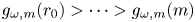
Suppose that $\omega >1$ and write $g(r)=g_{\omega,m}(r)$
 . We extend the domain of $g(r)$
 by setting $g(-1)=0$
 and $g(m+1)=\frac {g(m)}{\omega }$
 in keeping with (1.1). It is easy to prove that $g(r)$
 is a unimodal function c.f. [Reference Byun and Poznanović2, § 2]. Hence there exists some $r_0\in \{0,\,1,\,\ldots,\,m\}$
 that satisfies

As $g(-1)< g(0)=1$ and $\left (\frac {2}{\omega }\right )^m=g(m)>g(m+1)=\frac {2^m}{\omega ^{m+1}}$
 , both chains of inequalities are non-empty. The chains of inequalities (1.3) serve to define $r_0$
 .
.
We use theorem 1.1 to show that $r_0$ is commonly close to $r':=\lfloor \frac {m+2}{\omega +1}\rfloor$
 . We always have $r'\leqslant r_0$
 (by lemma 3.3) and though $r_0-r'$
 approaches $\frac {m}{2}$
 as $\omega$
 approaches 1 (see remark 4.4), if $\omega \geqslant \sqrt {3}$
 then $0\leqslant r_0 - r'\leqslant 1$
 by the next theorem.
Theorem 1.3 If $\omega \geqslant \sqrt {3}$ , $m\in \{0,\,1,\,\ldots \}$
 and $r':=\lfloor \frac {m+2}{\omega +1}\rfloor$
 , then $r_0\in \{r',\,r'+1\}$
 , that is

Sharp bounds for $Q$ seem powerful: they enable short and elementary proofs of results that previously required substantial effort. For example, our proof in [Reference Glasby and Paseman4, Theorem 1.1] for $\omega =2$
 of the formula $r_0=\lfloor \frac {m}{3}\rfloor +1$
 involved a lengthy argument, and our first proof of theorem 1.4 below involved a delicate induction. By this theorem there is a unique maximum, namely $r_0=r'=\lfloor \frac {m+2}{\omega +1}\rfloor$
 when $\omega \in \{3,\,4,\,5,\,\ldots \}$
 and $\omega \ne m+1$
 , c.f. remark 4.2. In particular, strict inequality $g_{\omega,m}(r'-1)< g_{\omega,m}(r')$
 holds.
Theorem 1.4 Suppose that $\omega \in \{3,\,4,\,5,\,\ldots \}$ and $r'=\lfloor \frac {m+2}{\omega +1}\rfloor$
 . Then

with equality if and only if $\omega =m+1$ .
.
Our motivation was to analyse $g_{\omega,m}(r)$ by using estimates for $Q$
 given by the generalized continued fraction in theorem 1.1. This gives tighter estimates than the method involving partial sums used in [Reference Glasby and Paseman4]. The plots of $y=g_{\omega,m}(r)$
 for $0\leqslant r\leqslant m$
 are highly asymmetrical if $\omega -1$
 and $m$
 are small. However, if $m$
 is large the plots exhibit an ‘approximate symmetry’ about the vertical line $r=r_0$
 (see figure 1). Our observation that $r_0$
 is close to $r'$
 for many choices of $\omega$
 was the starting point of our research.

Figure 1. Plots of $y=g_{\omega,24}(r)$ for $0\leqslant r\leqslant 24$
 with $\omega \in \{1,\,\frac 32,\,2,\,3\}$
 , and $y=g_{3,12}(r)$
Byun and Poznanović [Reference Byun and Poznanović2, Theorem 1.1] compute the maximizing input, call it $r^*$ , for the function $f_{m,a}(r):=(1+a)^{-r}\sum _{i=0}^r\binom{m}{i}a^i$
 where $a\in \{1,\,2,\,\ldots \}$
 . Their function equals $g_{\omega,m}(r)$
 only when $\omega =1+a=2$
 . Some of their results and methods are similar to those in [Reference Glasby and Paseman4] which studied the case $\omega =2$
 . They prove that $r^*=\lfloor \frac {a(m+1)+2}{2a+1}\rfloor$
 provided $m\not \in \{3,\,2a+4,\,4a+5\}$
 or $(a,\,m)\ne (1,\,12)$
 when $r^*=\lfloor \frac {a(m+1)+2}{2a+1}\rfloor -1$
 .
.
In Section 2 we prove theorem 1.1 and record approximations to our generalized continued fraction expansion. When $m$ is large, the plots of $y=g_{\omega,m}(r)$
 are reminiscent of a normal distribution with mean $\mu \approx \frac {m}{\omega +1}$
 . Section 3 proves key lemmas for estimating $r_0$
 , and applies theorem 1.1 to prove theorem 1.4. Non-integral values of $\omega$
 are considered in Section 4 where theorem 1.3 is proved. In Section 5 we estimate the maximum height $g(r_0)$
 using elementary methods and estimations, see lemma 5.1. A ‘statistical’ approximation to $s_m(r)$
 is given in remark 5.3, and it is compared in remark 5.4 to the ‘generalized continued fraction approximations’ of $s_m(r)$
 in proposition 2.3.
2. Generalized continued fraction formulas
In this section we prove theorem 1.1, namely that $Q:=\frac {r+1}{s_m(r)}\binom{m}{r+1}=a_0+{\mathcal {T}}_1$ where ${\mathcal {T}}_1=\mathcal{K}_{i=1}^r\frac {b_i}{a_i}$
 . The equality $s_m(r)=\frac {r+1}{a_0+{\mathcal {T}}_1}\binom{m}{r+1}$
 is noted in corollary 2.2.
A version of theorem 1.1(a) was announced in the SCS2022 Poster room, created to run concurrently with vICM 2022, see [Reference Paseman9].
Proof Proof of theorem 1.1
Set $R_{-1}=Q\,s_m(r)=(r+1)\binom{m}{r+1}=(m-r)\binom{m}{r}$ and
and

Clearly $R_0=s_m(r)$ , $R_{r+1}=0$
 and $R_j>0$
 for $0\leqslant j\leqslant r$
 . We will prove in the following paragraph that the quantities $R_j$
 , $a_j=m-2r+3j$
 , and $b_j=2j(r+1-j)$
 satisfy the following $r+1$
 equations, where the first equation (2.1) is atypical:


Assuming (2.2) is true, we prove by induction that ${\mathcal {T}}_{j}=R_{j}/R_{j-1}$ holds for $r+1\geqslant j\geqslant 1$
 . This is clear for $j=r+1$
 since ${\mathcal {T}}_{r+1}=R_{r+1}=0$
 . Suppose that $1\leqslant j\leqslant r$
 and ${\mathcal {T}}_{j+1}=R_{j+1}/R_{j}$
 holds. We show that ${\mathcal {T}}_{j}=R_{j}/R_{j-1}$
 holds. Using (2.2) and $R_j>0$
 we have $b_jR_{j-1}/R_j-a_j=R_{j+1}/R_j={\mathcal {T}}_{j+1}$
 . Hence $R_j/R_{j-1}=b_j/(a_j+{\mathcal {T}}_{j+1})={\mathcal {T}}_j$
 , completing the induction. Equation (2.1) gives $Q=R_{-1}/R_0=a_0+R_1/R_{0}=a_0+{\mathcal {T}}_1$
 as claimed. Since $R_j>0$
 for $0\leqslant j\leqslant r$
 , we have ${\mathcal {T}}_{j}=R_{j}/R_{j-1}>0$
 for $1\leqslant j\leqslant r$
 . This proves the first half of theorem 1.1(b), and the recurrence ${\mathcal {T}}_j=b_j/(a_j+{\mathcal {T}}_{j+1})$
 for $1\leqslant j\leqslant r$
 , proves part (a).
We now show that (2.1) holds. The identity $R_0=2^00!\sum _{k=0}^r\binom{m}{k}=s_m(r)$ gives
gives

As $(i+1)\binom{m}{i+1}=(m-i)\binom{m}{i}$ , we get $R_{-1}-a_0R_0=2\sum _{k=0}^{r-1}\binom{r-k}{1}\binom{m}{k}=R_1$
 .
.
We next show that (2.2) holds. In order to simplify our calculations, we divide by $C_{j}:= 2^j j!$ . Using $(j+1)\binom{r-k}{j+1}=(r-k-j)\binom{r-k}{j}$
 gives
gives

noting that the term with $k=r-j+1$ in the first sum is zero as $\binom{j-1}{j}=0$
 . Using the abbreviation $L=\sum _{k=0}^{r-j}(k-2r+3j)\binom{r-k}{j}\binom{m}{k}$
 and using the identity $j\binom{r-k}{j}=(r+1-j-k)\binom{r-k}{j-1}$
 gives
gives

However, $k\binom{m}{k}=(m-k+1)\binom{m}{k-1}$ , and therefore,

Thus

Hence $\frac {R_{j+1}}{C_{j}}=\frac {b_{j}R_{j-1}}{C_{j}}-\frac {a_{j}R_{j}}{C_{j}}$ for $1\leqslant j\leqslant r$
 . When $j=r$
 , our convention gives $R_{r+1}=0$
 . This proves part (b) and completes the proof of part (a).
Remark 2.1 View $m$ as an indeterminant, so that $r!s_m(r)$
 is a polynomial in $m$
 over ${\mathbb {Z}}$
 of degree $r$
 . The factorization $r!s_m(r)=\prod _{j=1}^r(a_j+{\mathcal {T}}_{j+1})$
 in corollary 1.2 involves the rational functions $a_j+{\mathcal {T}}_{j+1}$
 . However, theorem 1.1(b) gives ${\mathcal {T}}_{j+1}=\frac {R_{j+1}}{R_{j}}$
 , so that $a_j+{\mathcal {T}}_{j+1}=\frac {a_{j}R_{j}+R_{j+1}}{R_j}=\frac {b_{j}R_{j-1}}{R_j}$
 . This determines the numerator and denominator of the rational function $a_j+{\mathcal {T}}_{j+1}$
 , and explains why we have $\prod _{j=1}^r(a_j+{\mathcal {T}}_{j+1})= \frac {R_0}{R_r}\prod _{j=1}^rb_{j}=r!s_m(r)$
 . This is different from, but reminiscent of, the ratio $p_{j+1}/p_j$
 described on p. 26 of [Reference Olds8]. $\diamond$
Corollary 2.2 If $r,\,m\in {\mathbb {Z}}$ and $0< r< m$
 , then

If $r=0$ , then $s_m(r)=\frac {(r+1)\binom{m}{r+1}}{m-2r+{\mathcal {T}}_1}$
 is true, but ${\mathcal {T}}_1=\mathcal{K}_{i=1}^r\frac {2i(r+1-i)}{m-2r+3i}=0$
 .
.
We will need some additional tools such as proposition 2.3 and corollary 2.4 below in order to prove theorem 1.3.
Since $s_m(m-r)=2^m-s_m(r-1)$ approximating $s_m(r)$
 for $0\leqslant r\leqslant m$
 reduces to approximating $s_m(r)$
 for $0\leqslant r\leqslant \lfloor \frac {m}{2}\rfloor$
 . Hence the hypothesis $r<\frac {m+3}{2}$
 in proposition 2.3 and corollary 2.4 is not too restrictive. Proposition 2.3 generalizes [Reference Olds8, Theorem 3.3].
Let ${\mathcal {H}}_j:=\mathcal{K}_{i=1}^j\frac {b_i}{a_i}$ denote the $j$
 th head of the fraction $\mathcal{K}_{i=1}^r\frac {b_i}{a_i}$
 , where ${\mathcal {H}}_0=0$
 .
.
Proposition 2.3 Let $b_i=2i(r+1-i)$ and $a_i=m-2r+3i$
 for $0\leqslant i\leqslant r$
 . If $r<\frac {m+3}{2}$
 , then $a_0+{\mathcal {H}}_r=\frac {(r+1)\binom{m}{r+1}}{s_m(r)}$
 can be approximated using the following chain of inequalities

Proof. Note that $r$ equals either $2\lfloor r/2\rfloor$
 or $2\lfloor (r-1)/2\rfloor +1$
 , depending on its parity.
We showed in the proof of theorem 1.1 that $\frac {(r+1)\binom{m}{r+1}}{s_m(r)}=a_0+{\mathcal {H}}_r=a_0+\mathcal{K}_{i=1}^r\frac {b_i}{a_i}$ . Since $r<\frac {m+3}{2}$
 , we have $a_i>0$
 and $b_i>0$
 for $1\leqslant i\leqslant r$
 and hence $\frac {b_i}{a_i}>0$
 . A straightforward induction (which we omit) depending on the parity of $r$
 proves that ${\mathcal {H}}_0<{\mathcal {H}}_2<\cdots <{\mathcal {H}}_{2\lfloor r/2\rfloor }<{\mathcal {H}}_{2\lfloor (r-1)/2\rfloor +1}<\cdots <{\mathcal {H}}_3<{\mathcal {H}}_1$
 . For example, if $r=3$
 , then

proves ${\mathcal {H}}_0<{\mathcal {H}}_2<{\mathcal {H}}_3<{\mathcal {H}}_1$ as the tails are positive. Adding $a_0$
 proves the claim.
In asking whether $g_{\omega,m}(r)$ is a unimodal function, it is natural to consider the ratio $g_{\omega,m}(r+1)/g_{\omega,m}(r)$
 of successive terms. This suggests defining

We will prove in lemma 3.1 that $t(r)$ is a strictly decreasing function that determines when $g_{\omega,m}(r)$
 is increasing or decreasing, and $t_{m}(r_0-1)\geqslant \omega >t_{m}(r_0)$
 determines $r_0$
 .
.
Corollary 2.4 We have $m-2r\leqslant \frac {(r+1)\binom{m}{r+1}}{s_m(r)}$ for $r\geqslant 0$
 , and
, and

Hence $\frac {m+2}{r+1}\leqslant t_m(r)+1$ for $r\geqslant 0$
 , and
, and

Also $\frac {m+2}{r+1}< t_m(r)+1$ for $r>0$
 , and the above upper bound is strict for $1< r<\frac {m+3}{2}$
 .
.
Proof. We proved $Q=\frac {(r+1)\binom{m}{r}}{s_m(r)}=(m-2r)+\mathcal{K}_{i=1}^r\frac {2i(r+1-i)}{m-2r+3i}$ in theorem 1.1. Hence $m-2r=\frac {(r+1)\binom{m}{r+1}}{s_m(r)}$
 if $r=0$
 and $m-2r<\frac {(r+1)\binom{m}{r+1}}{s_m(r)}$
 if $1\leqslant r<\frac {m+3}{2}$
 by proposition 2.3. Clearly $m-2r<0\le \frac {(r+1)\binom{m}{r+1}}{s_m(r)}$
 if $\frac {m+3}{2}\le r\le m$
 . Similarly $\frac {(r+1)\binom{m}{r+1}}{s_m(r)}= m-2r+\frac {2r}{m-2r+3}$
 if $r=0,\,1$
 , and again proposition 2.3 shows that ${\frac {(r+1)\binom{m}{r+1}}{s_m(r)}< m-2r+\frac {2r}{m-2r+3}}$
 if $1< r<\frac {m+3}{2}$
 . The remaining inequalities (and equalities) follow similarly since $t_m(r)+1=2+\frac {\binom{m}{r+1}}{s_m(r)}$
 and $2+\frac {m-2r}{r+1}=\frac {m+2}{r+1}$
 .
.
3. Estimating the maximizing input $r_0$

Fix $\omega >1$ . In this section we consider the function $g(r)=g_{\omega,m}(r)$
 given by (1.1). As seen in table 1, it is easy to compute $g(r)$
 if $r$
 is near $0$
 or $m$
 . For $m$
 large and $r$
 near $0$
 , we have ‘sub-exponential’ growth $g(r)\approx \frac {m^r}{r!\omega ^r}$
 . Similarly for $r$
 near $m$
 , we have exponential decay $g(r)\approx \frac {2^m}{\omega ^r}$
 . The middle values require more thought.
Table 1. Values of $g_{w,m}(r)$

On the other hand, the plots $y=g(r)$ , $0\leqslant r\leqslant m$
 , exhibit a remarkable visual symmetry when $m$
 is large. The relation $s_m(m-r)=2^m-s_m(r-1)$
 and the distorting scale factor of $\omega ^{-r}$
 shape the plots. The examples in figure 1 show an approximate left–right symmetry about a maximizing input $r\approx \frac {m}{\omega +1}$
 . It surprised the authors that in many cases there exists a simple exact formula for the maximizing input (it is usually unique as corollary 3.2 suggests). In figure 1 we have used different scale factors for the $y$
 -axes. The maximum value of $g_{\omega,m}(r)$
 varies considerably as $\omega$
 varies (c.f. lemma 5.1), so we scaled the maxima (rounded to the nearest integer) to the same height.
Lemma 3.1 Recall that $g(r)=\omega ^{-r} s_m(r)$ by (1.1) and $t(r)=\frac {s_m(r+1)}{s_m(r)}$
 by (2.3).
(a) $t(r-1)>t(r)>\frac {m-r}{r+1}$
for $0\leqslant r\leqslant m$ where $t(-1):=\infty$;(b) $g(r)< g(r+1)$
if and only if $t(r)>\omega$;(c) $g(r)\leqslant g(r+1)$
if and only if $t(r)\geqslant \omega$;(d) $g(r)> g(r+1)$
if and only if $\omega > t(r)$;(e) $g(r)\geqslant g(r+1)$
if and only if $\omega \geqslant t(r)$;(f) if $\omega >1$
then some $r_0\in \{0,\,\ldots,\,m\}$ satisfies $t(r_0-1)\geqslant \omega > t(r_0)$, and this condition is equivalent to
\[ g(0)<\cdots < g(r_0-1)\leqslant g(r_0) \quad {\rm and}\quad g(r_0)>\cdots >g(m). \]


Proof. (a) We prove, using induction on $r$ , that $t(r-1)>t(r)>\binom{m}{r+1}/\binom{m}{r}$
 holds for $0\leqslant r\leqslant m$
 . These inequalities are clear for $r=0$
 as $\infty >m+1>m$
 . For real numbers $\alpha,\,\beta,\,\gamma,\,\delta >0$
 , we have $\alpha \delta -\beta \gamma >0$
 if and only if $\frac {\alpha }{\beta }>\frac {\alpha +\gamma }{\beta +\delta }>\frac {\gamma }{\delta }$
 ; that is, the mediant $\frac {\alpha +\gamma }{\beta +\delta }$
 of $\frac {\alpha }{\beta }$
 and $\frac {\gamma }{\delta }$
 lies strictly between $\frac {\alpha }{\beta }$
 and $\frac {\gamma }{\delta }$
 . If $0< r\leqslant m$
 , then by induction

Applying the ‘mediant sum’ to $t(r-1)=\frac {s_m(r)}{s_m(r-1)}>\frac {\binom{m}{r+1}}{\binom{m}{r}}$ gives
gives

Therefore $t(r-1)>t(r)>\binom{m}{r+1}/\binom{m}{r}=\frac {m-r}{r+1}$ completing the induction, and proving (a).
(b,c,d,e) The following are equivalent: $g(r)< g(r+1)$ ; $\omega s_m(r)< s_m(r+1)$
 ; and $\omega < t(r)$
 . The other claims are proved similarly by replacing < with $\leqslant$
 , >, $\geqslant$
 .
.
(f) Observe that $t(m)=\frac {s_m(m+1)}{s_m(m)}=\frac {2^m}{2^m}=1$ . By part (a), the function $y=t(r)$
 is decreasing for $-1\leqslant r\leqslant m$
 . Since $\omega >1$
 , there exists an integer $r_0\in \{0,\,\ldots,\,m\}$
 such that $\infty =t(-1)>\cdots >t(r_0-1)\geqslant \omega > t(r_0)>\cdots > t(m)=1$
 . By parts (b,c,d,e) an equivalent condition is $g(0)<\cdots < g(r_0-1)\leqslant g(r_0)$
 and $g(r_0)>\cdots >g(m)$
 .
.
The following is an immediate corollary of lemma 3.1(f).
Corollary 3.2 If $t(r_0-1)>\omega$ , then the function $g(r)$
 in (1.1) has a unique maximum at $r_0$
 . If $t(r_0-1)=\omega$
 , then $g(r)$
 has two equal maxima, one at $r_0-1$
 and one at $r_0$
 .
.
As an application of theorem 1.1 we show that the largest maximizing input $r_0$ for $g_{\omega,m}(r)$
 satisfies $\lfloor \frac {m+2}{\omega +1}\rfloor \leqslant r_0$
 . There are at most two maximizing inputs by corollary 3.2.
Lemma 3.3 Suppose that $\omega >1$ and $m\in {\mathbb {Z}}$
 , $m\geqslant 0$
 . If $r':=\lfloor \frac {m+2}{\omega +1}\rfloor$
 , then

if $r'>1$ or $\omega \ne m+1$
 .
.
Proof. The result is clear when $r'=0$ . If $r'=1$
 , then $r'\leqslant \frac {m+2}{\omega +1}$
 gives $\omega \leqslant m+1$
 or $g(0)\leqslant g(1)$
 . Hence $g(0)< g(1)$
 if $\omega \ne m+1$
 . Suppose that $r'>1$
 . By lemma 3.1(c,f) the chain $g(0)<\dots < g(r')$
 is equivalent to $g(r'-1)< g(r')$
 , that is $t(r'-1)> \omega$
 . However, $t(r'-1)+1>\frac {m+2}{r'}$
 by corollary 2.4 and $r'\leqslant \frac {m+2}{\omega +1}$
 implies $\frac {m+2}{r'}\geqslant \omega +1$
 . Hence $t(r'-1)+1>\omega +1$
 , so that $t(r'-1)> \omega$
 as desired.
Proof Proof of theorem 1.4
Suppose that $\omega \in \{3,\,4,\,\ldots \}$ . Then $g(0)<\dots < g(r'-1)\leqslant g(r')$
 by lemma 3.3 with strictness when $\omega \ne m+1$
 . If $\omega =m+1$
 , then $r'=\lfloor \frac {m+2}{\omega +1}\rfloor =1$
 and $g(0)=g(1)$
 as claimed. It remains to show that $g(r')>g(r'+1)>\cdots >g(m)$
 . However, we need only prove that $g(r')> g(r'+1)$
 by lemma 3.1(f), or equivalently $\omega > t(r')$
 by lemma 3.1(d).
Clearly $\omega \geqslant 3$ implies $r'\leqslant \frac {m+2}{\omega +1}\leqslant \frac {m+2}{4}$
 . As $0\leqslant r'<\frac {m+3}{2}$
 , corollary 2.4 gives

Hence $\omega +1> t(r')+1$ holds if $\omega +1> \frac {m+2}{r'+1}+\frac {2r'}{(r'+1)(m-2r'+3)}$
 . Since $\omega +1$
 is an integer, we have $m+2=r'(\omega +1)+c$
 where $0\leqslant c\leqslant \omega$
 . It follows from $0\leqslant r'\leqslant \frac {m+2}{4}$
 that $\frac {2r'}{m-2r'+3}<1$
 . This inequality and $m+2\leqslant r'(\omega +1)+\omega$
 gives
gives

Thus $\omega +1>\frac {m+2}{r'+1}+\frac {2r'}{(r'+1)(m-2r'+3)}\geqslant t(r')+1$ , so $\omega >t(r')$
 as required.
Remark 3.4 The proof of theorem 1.4 can be adapted to the case $\omega =2$ . If $m+2=3r'+c$
 where $c\leqslant \omega -1=1$
 , then $\frac {2r'}{m-2r'+3}=\frac {2r'}{r'+c+1}<2$
 , and if $c=\omega =2$
 , then a sharper ${\mathcal {H}}_2$
 -bound must be used. This leads to a much shorter proof than [Reference Glasby and Paseman4, Theorem 1.1]. $\diamond$
4. Non-integral values of $\omega$

In this section, we prove that the maximum value of $g(r)$ is $g(r')$
 or $g(r'+1)$
 if $\omega \geqslant \sqrt {3}$
 . Before proving this result (theorem 1.3), we shall prove two preliminary lemmas.
Lemma 4.1 Suppose that $\omega >1$ and $r':=\lfloor \frac {m+2}{\omega +1}\rfloor$
 . If $\frac {m+2}{r'+1}\geqslant \sqrt {3}+1$
 , then

Proof. It suffices, by lemma 3.1(f) and lemma 3.3 to prove that $g(r'+1)>g(r'+2)$ . The strategy is to show $\omega >t(r'+1)$
 , that is $\omega +1>t(r'+1)+1$
 . However, $\omega +1>\frac {m+2}{r'+1}$
 , so it suffices to prove that $\frac {m+2}{r'+1}\geqslant t(r'+1)+1$
 . Since $r'+1\leqslant \frac {m+2}{\sqrt {3}+1}<\frac {m+2}{2}$
 , we can use corollary 2.4 and just prove that $\frac {m+2}{r'+1}\geqslant \frac {m+2}{r'+2}+\frac {2r'+2}{(r'+2)(m-2r'+1)}$
 . This inequality is equivalent to $\frac {m+2}{r'+1}\geqslant \frac {2r'+2}{m-2r'+1}$
 . However, $\frac {m+2}{r'+1}\geqslant \sqrt {3}+1$
 , so we need only show that $\sqrt {3}+1\geqslant \frac {2(r'+1)}{m-2r'+1}$
 , or equivalently $m-2r'+1\geqslant (\sqrt {3}-1)(r'+1)$
 . This is true since $\frac {m+2}{r'+1}\geqslant \sqrt {3}+1$
 implies $m-2r'+1\geqslant (\sqrt {3}-1)r'+\sqrt {3}>(\sqrt {3}-1)(r'+1)$
 .
.
Remark 4.2 The strict inequality $g(r'-1)< g(r')$ holds by lemma 3.3 if $r'>1$
 or $\omega \ne m+1$
 . It holds vacuously for $r'=0$
 . Hence adding the additional hypothesis that $\omega \ne m+1$
 if $r'=1$
 to lemma 4.1 (and theorem 1.3), we may conclude that the inequality $g(r'-1)\leqslant g(r')$
 is strict.
Remark 4.3 In lemma 4.1, the maximum can occur at $r'+1$ . If $\omega =2.5$
 and $m=8$
 , then $r'=\lfloor \frac {10}{3.5}\rfloor =2$
 and $\frac {m+2}{r'+1}=\frac {10}{3}\geqslant \sqrt {3}+1$
 however $g_{2.5,8}(2)=\frac {740}{125}< \frac {744}{125}=g_{2.5,8}(3)$
 . $\diamond$
Remark 4.4 The gap between $r'$ and the largest maximizing input $r_0$
 can be arbitrarily large if $\omega$
 is close to 1. For $\omega >1$
 , we have $r'=\lfloor \frac {m+2}{\omega +1}\rfloor <\frac {m+2}{2}$
 . If $1<\omega \leqslant \frac {1}{1-2^{-m}}$
 , then $g(m-1)\leqslant g(m)$
 , so $r_0=m$
 . Hence $r_0-r'>\frac {m-2}{2}$
 .
.
Remark 4.5 Since $r'\leqslant \lfloor \frac {m+2}{\omega +1}\rfloor < r'+1$ , we see that $r'+1\approx \frac {m+2}{\omega +1}$
 , so that $\frac {m+2}{r'+1}\approx \omega +1$
 . Thus lemma 4.1 suggests that if $\omega \gtrsim \sqrt {3}$
 , then $g_{\omega,m}(r)$
 may have a maximum at $r'$
 or $r'+1$
 . This heuristic reasoning is made rigorous in theorem 1.3. $\diamond$
Remark 4.6 Theorem 1.1 can be rephrased as $t_m(r)=\frac {s_m(r+1)}{s_m(r)}=\frac {m-r+1}{r+1}+\frac {{\mathcal {K}}_m(r)}{r+1}$ where
where

The following lemma repeatedly uses the expression $\omega >t_m(r+1)$ . This is equivalent to $\omega >\frac {m-r}{r+2}+\frac {{\mathcal {K}}_m(r+1)}{r+2}$
 , that is $(\omega +1)(r+2)>m+2+{\mathcal {K}}_m(r+1)$
 . $\diamond$
Lemma 4.7 Let $m\in \{0,\,1,\,\ldots \}$ and $r'=\lfloor \frac {m+2}{\omega +1}\rfloor$
 . If any of the following three conditions are met, then $g_{\omega,m}(r'+1)>\cdots >g_{\omega,m}(m)$
 holds: (a) $\omega \geqslant 2$
 , or (b) $\omega \geqslant \frac {1+\sqrt {97}}{6}$
 and $r'\ne 2$
 , or (c) $\omega \geqslant \sqrt {3}$
 and $r'\not \in \{2,\,3\}$
 .
.
Proof. The conclusion $g_{\omega,m}(r'+1)>\cdots >g_{\omega,m}(m)$ holds trivially if $r'+1\geqslant m$
 . Suppose henceforth that $r'+1< m$
 . Except for the excluded values of $r',\,\omega$
 , we will prove that $g_{\omega,m}(r'+1)>g_{\omega,m}(r'+2)$
 holds, as this implies $g_{\omega,m}(r'+1)>\cdots >g_{\omega,m}(m)$
 by lemma 3.1(f). Hence we must prove that $\omega >t_m(r'+1)$
 by lemma 3.1(d).
Recall that $r'\leqslant \frac {m+2}{\omega +1}< r'+1$ . If $r'=0$
 , then $m+2<\omega +1$
 , that is $\omega >m+1>t(1)$
 as desired. Suppose now that $r'=1$
 . There is nothing to prove if $m=r'+1=2$
 . Assume that $m>2$
 . Since $m+2<2(\omega +1)$
 , we have $2< m<2\omega$
 . The last line of remark 4.6 and (4.1) give the desired inequality:

In summary, $g_{\omega,m}(r'+1)>\cdots >g_{\omega,m}(m)$ holds for all $\omega >1$
 if $r'\in \{0,\,1\}$
 .
.
We next prove $g_{\omega,m}(r'+1)>g_{\omega,m}(r'+2)$ , or equivalently $\omega >t_m(r'+1)$
 for $r'$
 large enough, depending on $\omega$
 . We must prove that $(\omega +1)(r'+2)>m+2+\mathcal{K}_m(r'+1)$
 by remark 4.6. Writing $m+2=(\omega +1)(r'+\varepsilon )$
 where $0\leqslant \varepsilon <1$
 , our goal, therefore, is to show $(\omega +1)(2-\varepsilon )>{\mathcal {K}}_m(r'+1)$
 . Using (4.1) gives

where ${\mathcal {T}}>0$ by theorem 1.1 as $r'>0$
 . Rewriting the denominator using

our goal $(\omega +1)(2-\varepsilon )>{\mathcal {K}}_m(r'+1)$ becomes

Dividing by $(2-\varepsilon )(r'+1)$ and rearranging gives

This inequality may be written $(\omega ^2-1)+\lambda >\frac {2}{2-\varepsilon }+\mu (1-\varepsilon )$ where $\lambda =\frac {(\omega +1)(1+{\mathcal {T}})}{r'+1}>0$
 and $\mu =\frac {(\omega +1)^2}{r'+1}>0$
 . We view $f(\varepsilon ):=\frac {2}{2-\varepsilon }+\mu (1-\varepsilon )$
 as a function of a real variable $\varepsilon$
 where $0\leqslant \varepsilon <1$
 . However, $f(\varepsilon )$
 is concave as the second derivative $f''(\varepsilon )=\frac {4}{(2-\varepsilon )^3}$
 is positive for $0\leqslant \varepsilon <1$
 . Hence the maximum value occurs at an end point: either $f(0)=1+\mu$
 or $f(1)=2$
 . Therefore, it suffices to prove that $(\omega ^2-1)+\lambda >\max \{2,\,1+\mu \}$
 .
.
If $2\geqslant 1+\mu$ , then the desired bound $(\omega ^2-3)+\lambda >0$
 holds as $\omega \geqslant \sqrt {3}$
 . Suppose now that $2<1+\mu$
 . We must show $(\omega ^2-1)+\lambda >1+\mu$
 , that is $\omega ^2-2>\mu -\lambda =\frac {(\omega +1)(\omega -{\mathcal {T}})}{r'+1}$
 . Since ${\mathcal {T}}>0$
 , a stronger inequality (that implies this) is $\omega ^2-2\geqslant \frac {(\omega +1)\omega }{r'+1}$
 . The (equivalent) quadratic inequality $r'\omega ^2-\omega -2(r'+1)\geqslant 0$
 in $\omega$
 is true provided $\omega \geqslant \frac {1+\sqrt {1+8r'(r'+1)}}{2r'}$
 . This says $\omega \geqslant 2$
 if $r'=2$
 , and $\omega \geqslant \frac {1+\sqrt {97}}{6}$
 if $r'=3$
 . If $r'\geqslant 4$
 , we have

The conclusion now follows from the fact that $2>\frac {1+\sqrt {97}}{6} >\sqrt {3}$ .
.
Proof Proof of theorem 1.3
By lemma 4.1 it suffices to show that $g(r'+1)>g(r'+2)$ holds when $r'+1< m$
 and $\omega \geqslant \sqrt {3}$
 . By lemma 4.7(a), we can assume that $\sqrt {3}\leqslant \omega <2$
 and $r'\in \{2,\,3\}$
 . For these choices of $\omega$
 and $r'$
 , we must show that $\omega >t_m(r'+1)$
 by lemma 3.1 for all permissible choices of $m$
 . Since $(\omega +1)r'\leqslant m+2<(\omega +1)(r'+1)$
 , when $r'=2$
 we have $5<2(\sqrt {3}+1)\leqslant m+2<9$
 so that $4\leqslant m\leqslant 6$
 . However, $t_m(3)$
 equals $\tfrac {16}{15},\,\tfrac {31}{26},\,\tfrac {19}{14}$
 for these values of $m$
 . Thus $\sqrt {3}>t_m(3)$
 holds as desired. Similarly, if $r'=3$
 , then $8<3(\sqrt {3}+1)\leqslant m+2<12$
 so that $7\leqslant m\leqslant 9$
 . In this case $t_m(4)$
 equals $\tfrac {40}{33},\,\tfrac {219}{163},\,\tfrac {191}{128}$
 for these values of $m$
 . In each case $\sqrt {3}>t_m(4)$
 , so the proof is complete.
Remark 4.8 We place remark 4.4 in context. The conclusion of theorem 1.3 remains true for values of $\omega$ smaller than $\sqrt {3}$
 and not ‘too close to 1’ and $m$
 is ‘sufficiently large’. Indeed, by adapting the proof of lemma 4.7 we can show there exists a sufficiently large integer $d$
 such that $m > d^4$
 and $\omega > 1 + \frac {1}{d}$
 implies $g(r'+d) > g(r'+d+1)$
 . This shows that $r' \leqslant r_0 \leqslant r' +d$
 , so $r_0-r'\leqslant d$
 . We omit the technical proof of this fact. $\diamond$
Remark 4.9 The sequence, $a_0+{\mathcal {H}}_1,\,\ldots,\,a_0+{\mathcal {H}}_r$ terminates at $\frac {r+1}{s_m(r)}\binom{m}{r+1}$
 by theorem 1.1. We will not comment here on how quickly the alternating sequence in proposition 2.3 converges when $r<\frac {m+3}{2}$
 . If $r=m$
 , then $a_0=-m$
 and $\frac {m+1}{s_m(m+1)}\binom{m}{m+1}=0$
 , so theorem 1.1 gives the curious identity ${\mathcal {H}}_m=\mathcal{K}_{i=1}^m\frac {2i(m+1-i)}{3i-m}=m$
 . If $\omega$
 is less than $\sqrt {3}$
 and ‘not too close to 1’, then we believe that $r_0$
 is approximately $\lfloor \frac {m+2}{\omega +1}+ \frac {2}{\omega ^2 -1}\rfloor$
 , c.f. remark 4.8.
5. Estimating the maximum value of $g_{\omega,m}(r)$

In this section we relate the size of the maximum value $g_{\omega,m}(r_0)$ to the size of the binomial coefficient $\binom{m}{r_0}$
 . In the case that we know a formula for a maximizing input $r_0$
 , we can readily estimate $g_{\omega,m}(r_0)$
 using approximations, such as [Reference Stănică10], for binomial coefficients.
Lemma 5.1 The maximum value $g_{\omega,m}(r_0)$ of $g_{\omega,m}(r)$
 , $0\leqslant r\leqslant m$
 , satisfies

Proof. Since $g(r_0)$ is a maximum value, we have $g(r_0-1)\leqslant g(r_0)$
 . This is equivalent to $(\omega -1)s_m(r_0-1)\leqslant \binom{m}{r_0}$
 as $s_m(r_0)=s_m(r_0-1)+\binom{m}{r_0}$
 . Adding $(\omega -1)\binom{m}{r_0}$
 to both sides gives the equivalent inequality $(\omega -1) s_m(r_0)\leqslant \omega \binom{m}{r_0}$
 . This proves the upper bound.
Similar reasoning shows that the following are equivalent: (a) $g(r_0)> g(r_0+1)$ ; (b) $(\omega -1)s_m(r_0)> \binom{m}{r_0+1}$
 ; and (c) $g_{\omega,m}(r_0)>\frac {1}{(\omega -1)\omega ^{r_0}}\binom{m}{r_0+1}$
 .
.
In theorem 1.3 the maximizing input $r_0$ satisfies $r_0=r'+d$
 where $d\in \{0,\,1\}$
 . In such cases when $r_0$
 and $d$
 are known, we can bound the maximum $g_{\omega,m}(r_0)$
 as follows.
Corollary 5.2 Set $r' := \lfloor \frac {m+2}{\omega +1}\rfloor$ and $k := m+2 - (\omega +1)r'$
 . Suppose that $r_0 = r'+d$
 and $G=\frac {1}{(\omega -1)\omega ^{r_0-1}}\binom{m}{r_0}$
 . Then

Proof. By lemma 3.3, $r_0 = r'+d$ where $d\in \{0,\,1,\,\ldots \}$
 . Since $r' = \lfloor \frac {m+2}{\omega +1}\rfloor$
 , we have $m+2 = (\omega +1)r'+k$
 where $0\leqslant k< \omega +1$
 . The result follows from lemma 5.1 and $m = (\omega +1)(r_0-d)+k-2$
 as $\binom{m}{r_0+1}=\frac {m-r_0}{r_0+1}\binom{m}{r_0}$
 and $\frac {m-r_0}{r_0+1}$
 equals

The following remark is an application of the Chernoff bound, c.f. [Reference Worsch11, Section 4]. Unlike theorem 1.1, it requires the cumulative distribution function $\Phi (x)$ , which is a non-elementary integral, to approximate $s_m(r)$
 . It seems to give better approximations only for values of $r$
 near $\frac {m}{2}$
 , see remark 5.4.
Remark 5.3 We show how the Berry–Esseen inequality for a sum of binomial random variables can be used to approximate $s_m(r)$ . Let $B_1,\,\ldots,\,B_m$
 be independent identically distributed binomial variables with a parameter $p$
 where $0< p<1$
 , so that $P(B_i=1)=p$
 and $P(B_i=0)=q:= 1-p$
 . Let $X_i:= B_i-p$
 and $X:=\frac {1}{\sqrt {mpq}}(\sum _{i=1}^m X_i)$
 . Then

Hence $E(X)=\frac {1}{\sqrt {mpq}}(\sum _{i=1}^m E(X_i))=0$ and $E(X^2)=\frac {1}{mpq}(\sum _{i=1}^m E(X_i^2))=1$
 . By [Reference Nagaev and Chebotarev7, Theorem 2] the Berry–Esseen inequality applied to $X$
 states that

where the constant $C:= 0.4215$ is close to the lower bound $C_0=\frac {10+\sqrt {3}}{6\sqrt {2\pi }}=0.4097\cdots$
 and $\Phi (x)=\frac {1}{\sqrt {2\pi }}\int _{-\infty }^x e^{-t^2/2}\,dt=\frac {1}{2}\left (1+{\rm erf}\left (\frac {x}{\sqrt {2}}\right )\right )$
 is the cumulative distribution function for standard normal distribution.
Writing $B=\sum _{i=1}^mB_i$ we have $P(B\leqslant b)=\sum _{i=0}^{\lfloor b\rfloor }\binom{m}{i}p^iq^{m-i}$
 for $b\in {\mathbb {R}}$
 . Thus $X=\frac {B-mp}{\sqrt {mpq}}$
 and $x=\frac {b-mp}{\sqrt {mpq}}$
 satisfy

Setting $p=q=\tfrac {1}{2}$ , and taking $b=r\in \{0,\,1,\,\ldots,\,m\}$
 shows
shows

Remark 5.4 Let $a_0+{\mathcal {H}}_k$ be the generalized continued fraction approximation to $\frac {(r+1)\binom{m}{r+1}}{s_m(r)}$
 suggested by theorem 1.1, where ${\mathcal {H}}_k:=\mathcal{K}_{i=1}^k\frac {b_i}{a_i}$
 , and $k$
 is the depth of the generalized continued fraction. We compare the following two quantities:

The sign of $e_{m,r,k}$ is governed by the parity of $k$
 by proposition 2.3. We shall assume that $r\leqslant \frac {m}{2}$
 . As $\frac {2^m}{s_m(r)}$
 ranges from $2^m$
 to about 2 as $r$
 ranges from 0 to $\lfloor \frac {m}{2}\rfloor$
 , it is clear that the upper bound for $E_{m,r}$
 will be huge unless $r$
 satisfies $\frac {m-\varepsilon }{2}\le r\le \frac {m}{2}$
 where $\varepsilon$
 is ‘small’ compared to $m$
 . By contrast, the computer code [Reference Glasby3] verifies that the same is true for $E_{m,r}$
 , and shows that $|e_{m,r,k}|$
 is small, even when $k$
 is tiny, when $0\le r<\frac {m-\varepsilon }{2}$
 , see table 2. Hence the ‘generalized continued fraction’ approximation to $s_m(r)$
 is complementary to the ‘statistical’ approximation, as shown in table 2. The reader can extend table 2 by running the code [Reference Glasby3] written in the Magma [Reference Bosma, Cannon and Playoust1] language, using the online calculator http://magma.maths.usyd.edu.au/calc/, for example.
Table 2. Upper bounds for $|e_{m,r,k}|$ and $E_{m,r}$
 for $m=10^4$

Acknowledgements
SPG received support from the Australian Research Council Discovery Project Grant DP190100450. GRP thanks his family, and SPG thanks his mother.


