1 Introduction
Studies on the electoral consequences of natural disasters have examined whether voters issue blanket electoral punishment to incumbent politicians in the wake of such disasters, or whether they assess the response of incumbents and reward or punish based on the quality of relief efforts. Studying natural disasters—random events that are exogenous to actions taken by elected officials—is valuable because it provides insight into the logic (or lack thereof) behind retrospective voting.Footnote 1 That is, if voters punish politicians for the effects of random events without incorporating those officials’ responses, the accountability mechanism of elections is weakened.
Studies of the effects of disaster and relief have come to contradictory conclusions. Achen and Bartels (Reference Achen and Bartels2002, Reference Achen and Bartels2016) established a foundation for the study of “blind retrospection” by investigating the electoral consequences of shark attacks along the New Jersey shore in 1916, droughts and floods in twenty-six presidential elections across the 20th century, and droughts and floods in the 2000 presidential election. Across these cases, they find evidence that citizens punish incumbent party candidates for random events outside of their control.
In contrast, other research suggests that voters represent an “attentive electorate”, capable of assigning praise and blame after a natural disaster by incorporating not just the effects of disasters but also subsequent relief operations. Healy and Malhotra (Reference Healy and Malhotra2009) find no evidence that disaster damage influences presidential vote share but do uncover a relationship between relief spending and support for the incumbent party. Similarly, Healy and Malhotra (Reference Healy and Malhotra2010) and Gasper and Reeves (Reference Gasper and Reeves2011) find voters punish incumbent presidents for damage from severe weather but that positive electoral effects of disaster declarations overwhelm the negative effects of the disaster itself. A key difference between these findings relates to the inclusion of relief spending as a variable: studies that account for relief efforts generally find that voters balance their assessment of disaster and subsequent relief.
Whether and how voters respond to disaster relief, however, is likely to be a product of their expectations regarding how the state should respond, a perspective that should vary across time and space.Footnote 2 For example, voters who live in a country with a highly active government will have different expectations regarding government relief than voters who live in a country with a less active government. These expectations are likely to depend on voters’ understanding of the state’s role at the time of the disaster.
Studies that assess the attentive electorate have covered differentiation across “space”—that is, across countries in the modern political era. In addition to studies that focus on the United States, a considerable literature also examines natural disaster and relief operations in other countries (Bechtel and Hainmueller Reference Bechtel and Hainmueller2011; Cole et al. Reference Cole, Healy and Werker2012; Fair et al. Reference Fair, Kuhn, Malhotra and Shapiro2013; Gallego Reference Gallego2012). These comparative studies find that voters incorporate government relief in their response to natural disasters and that, in at least some cases, natural disasters can be an electoral boon to incumbent politicians.
Differentiation across time, however, has not been studied to the same extent. While Achen and Bartels study some cases in the pre-New Deal United States (such as the 1916 shark attacks), research that examines attentive retrospection has focused exclusively on the post-New Deal era. This is concerning because, as the federal government has expanded dramatically over time, it has likely shaped voters’ perception of what the government should do, adjusting citizen expectations of state action. While the federal government has always been involved in (disaster) relief in some form (Dauber Reference Dauber2013), national politicians in the pre-New Deal era generally agreed that relief of hardship was the responsibility of state and local governments (Sundquist Reference Sundquist1983).Footnote 3 Thus, while voters in the post-New Deal era may have come to expect the federal government to provide aid in response to disasters, the same may not be true for voters in the early 20th century. To the extent that voters held different expectations in the pre-New Deal era, they may have held elected officials to different standards as well.
We contribute to this fast-growing literature by estimating the net electoral effect of disaster and relief in a single case of catastrophic flooding: the 1927 Mississippi Flood. This case is particularly interesting because (a) relief was provided on a then unprecedented scale and (b) 1928 Republican presidential candidate Herbert Hoover was responsible for the distribution of aid. Using county-level data on the severity of damage and the extent of the government’s response and both difference-in-differences and synthetic control models, we estimate the effect of a disaster that was—by most measures—the most damaging river flood in US history. Contrary to studies that find support for the attentive retrospection hypothesis, we find that the flood cost Hoover 10.8 percentage points in affected counties, despite his close association with the relief efforts.
2 The Great Mississippi Flood and the 1928 Presidential Election in the South
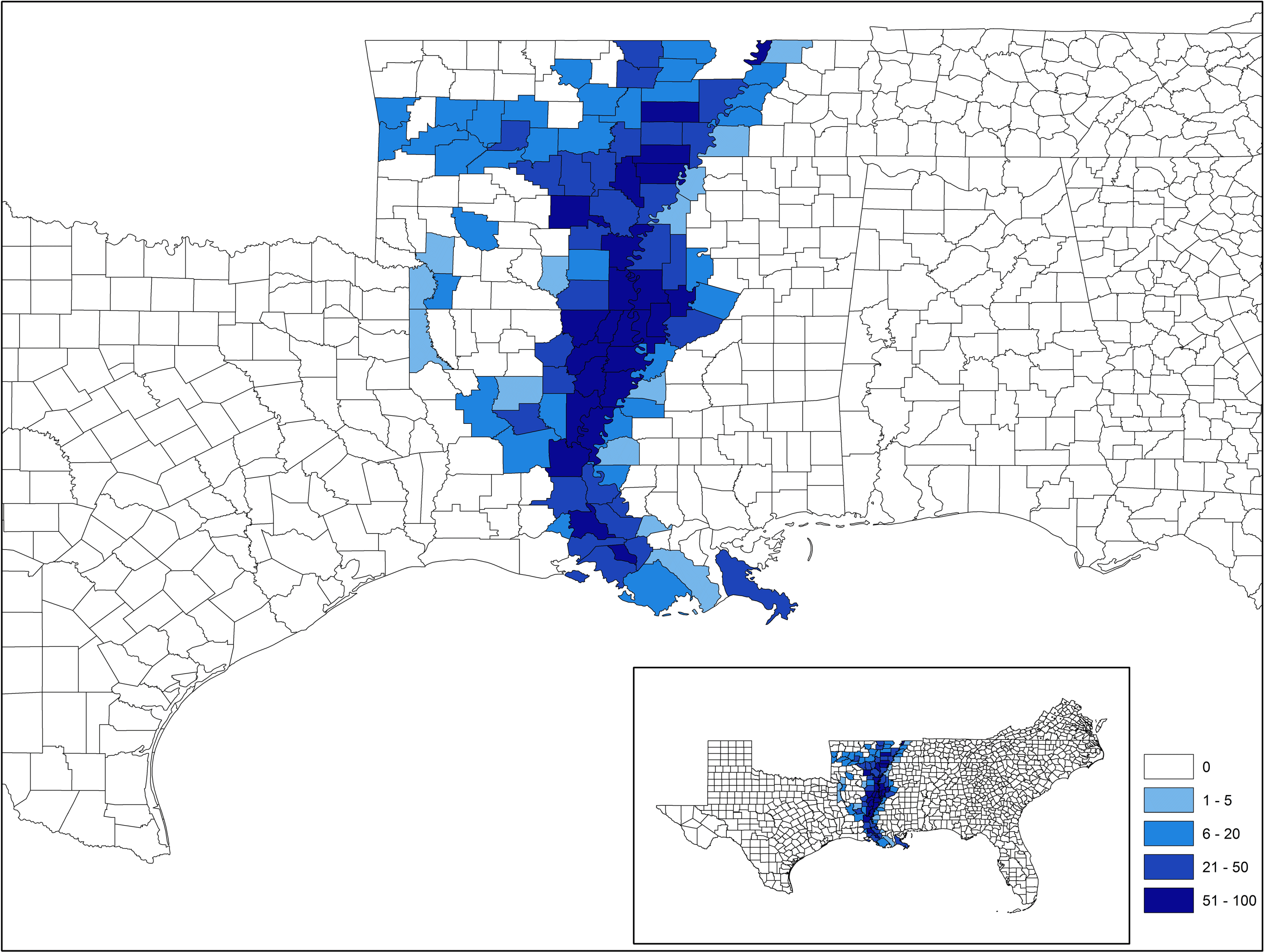
The Great Mississippi Flood of 1927 remains one of the largest natural disasters in American history. In the spring of 1927, a period of unusually heavy rainfall combined with significant deforestation resulted in the bursting of levees and major flooding in the Mississippi river valley (Daniel Reference Daniel1977). The flood’s devastation was unprecedented: over 26,000 square miles of land in 170 counties in Illinois, Kentucky, and—in particular—Tennessee, Arkansas, Mississippi, and Louisiana were flooded, and more than 750,000 people were forced to flee their homes (Spencer Reference Spencer1994; Kosar Reference Kosar2005). As Figure 1 illustrates, the flooding was particularly severe in Mississippi and Louisiana, with a considerable number of counties directly along the Mississippi River flooded entirely.

Figure 1. Flood severity by county during the Great Mississippi Flood of 1927. The percent of population affected by the Mississippi Flood, as reported by the Red Cross, across counties. More heavily flooded counties are shaded more darkly.
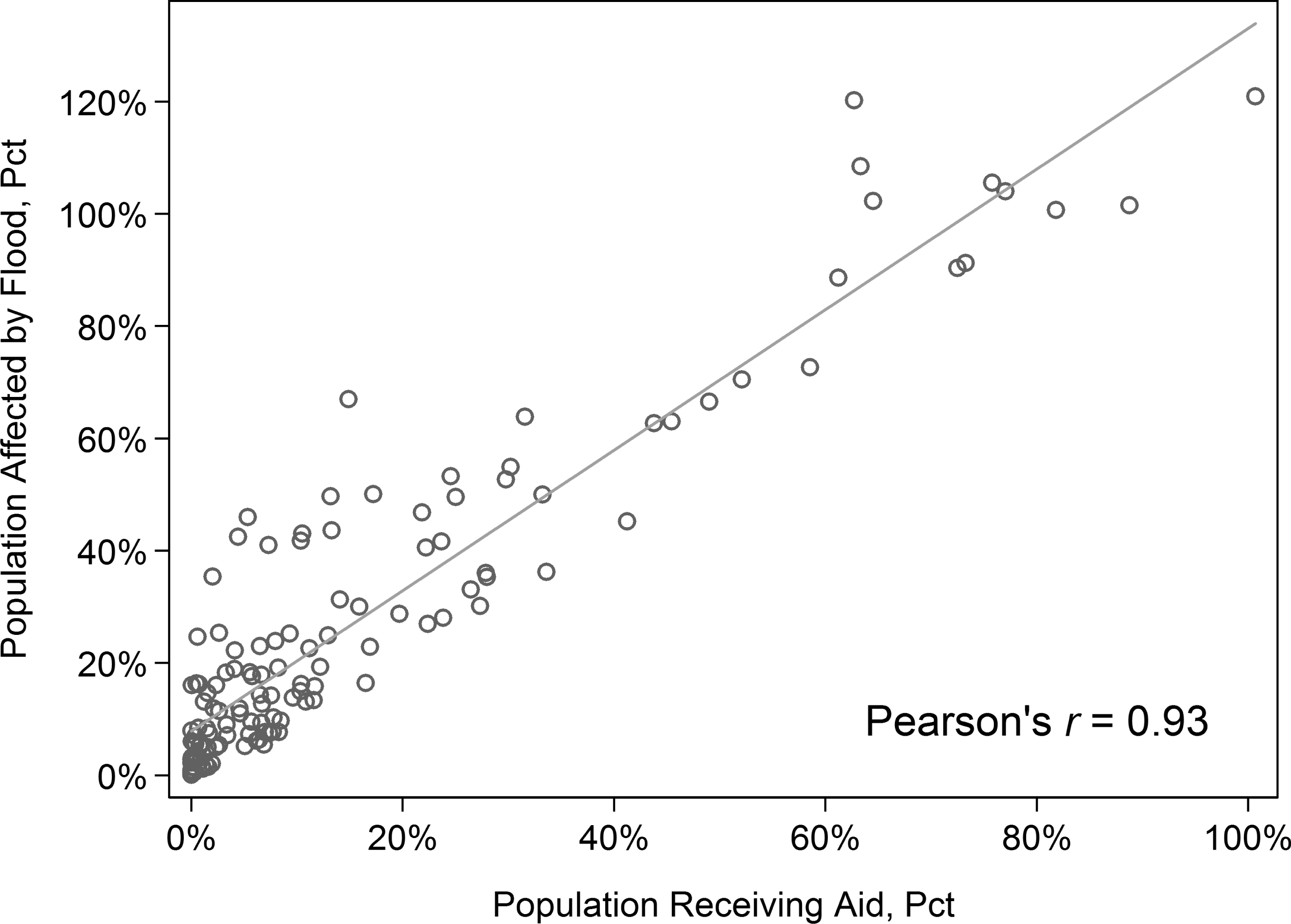
The flood was followed by a major relief operation organized by Republican President Calvin Coolidge’s administration.Footnote 4 The head of this operation was Herbert Hoover, then Secretary of Commerce and the GOP presidential nominee-to-be for 1928 (Barry Reference Barry1997, 240). Under Hoover’s leadership, more than 120,000 families across the South received Red Cross aid. Overall, the relief effort provided $32 million to the affected areas (Kosar Reference Kosar2005; Daniel Reference Daniel1977),Footnote 5 equivalent to $438 million in 2015 dollars. Importantly, the distribution of relief funds was generally seen as efficient and fair-minded: Figure 2 illustrates the strong correlation between flood damage and flood relief at the county level.Footnote 6 Compared to many other cases in the literature, this close correlation allows us to eliminate concerns regarding politically motivated relief distribution (Gallego Reference Gallego2012; Reeves Reference Reeves2011).

Figure 2. The correlation between flood severity and relief aid for treated counties in the US South (
![]() $n=98$
).
$n=98$
).
Hoover was also the public face of the relief operation, and made numerous site visits throughout the summer and fall of 1927. Newspapers and magazines reported on these visits, portraying Hoover as directly responsible for the relief efforts,Footnote 7 and local officials expressed their appreciation for the aid they received.Footnote 8 Hoover also referred to his role often throughout 1928, and his campaign created a film, entitled “Herbert Hoover, Master of Emergencies,” which showcased his humanitarian work during World War I and following the 1927 flood.Footnote 9
The Mississippi Flood thus offers a good test to assess the net effect of disaster and relief on an important election in the pre-New Deal United States. The disaster itself was significant, affecting a swath of voters across the American South. Relief efforts were considerable as well, and relief aid appears to have been distributed according to need. Finally, the Republican standard-bearer in 1928, Hoover, was visibly in charge of operations, making the link between politician and relief distribution particularly strong in this case.
3 Research Design
We focus our analysis on southern counties, among which 98 of 1,007 in our data experienced some flooding.Footnote
10
Our treatment variable is the percentage of individuals affected by the flood in each county
![]() $i$
, as documented by the Red Cross in their post-disaster report.Footnote
11
Since in this particular case disaster severity and aid are highly correlated (Figure 2), the measure of disaster damage includes the effect of both the natural disaster and subsequent relief efforts. In examining the 1927 Mississippi Flood, we can, therefore, assess the net effect by including only one measure in a statistical model. Because we expect the effect of flooding to vary with flood intensity, we bin this continuous treatment variable into a set of dummy variables representing varying levels of flood severity. We utilize a difference-in-differences approach, modeling the difference in Republican vote share between 1928 and 1924,
$i$
, as documented by the Red Cross in their post-disaster report.Footnote
11
Since in this particular case disaster severity and aid are highly correlated (Figure 2), the measure of disaster damage includes the effect of both the natural disaster and subsequent relief efforts. In examining the 1927 Mississippi Flood, we can, therefore, assess the net effect by including only one measure in a statistical model. Because we expect the effect of flooding to vary with flood intensity, we bin this continuous treatment variable into a set of dummy variables representing varying levels of flood severity. We utilize a difference-in-differences approach, modeling the difference in Republican vote share between 1928 and 1924,
![]() $v_{1928}^{i}-v_{1924}^{i}$
, as a function of a vector of covariates
$v_{1928}^{i}-v_{1924}^{i}$
, as a function of a vector of covariates
![]() $\unicode[STIX]{x1D6FE}$
, and a vector of treatment dummies,
$\unicode[STIX]{x1D6FE}$
, and a vector of treatment dummies,
![]() $\unicode[STIX]{x1D6FF}$
,
$\unicode[STIX]{x1D6FF}$
,
Note that we vary the number and construction of treatment dummies in several different specifications: we group all treated counties into a single treatment category; we split counties into three or five quantiles based on flood severity; and we also make subjective judgments regarding cutpoints in the treatment variable. The latter approach yields four categories, in which the percent of population impacted ranges from 0.1% to 5%, 5% to 20%, 20% to 50%, and 50% and up, respectively.
4 Results
We report the primary results, focused on the coefficient
![]() $\unicode[STIX]{x1D703}$
, in Figure 3. In each specification, we include the percent black from the 1920 US Census and a measure of county-level Protestantism, to control for the differential impact of Democratic presidential candidate Al Smith’s Catholicism across counties with different religious leanings.Footnote
12
Figure 3 plots coefficient estimates and 95% confidence intervals for our treatment dummies across specifications, with more heavily flooded categories always appearing lower on the graph’s
$\unicode[STIX]{x1D703}$
, in Figure 3. In each specification, we include the percent black from the 1920 US Census and a measure of county-level Protestantism, to control for the differential impact of Democratic presidential candidate Al Smith’s Catholicism across counties with different religious leanings.Footnote
12
Figure 3 plots coefficient estimates and 95% confidence intervals for our treatment dummies across specifications, with more heavily flooded categories always appearing lower on the graph’s
![]() $y$
-axis.
$y$
-axis.
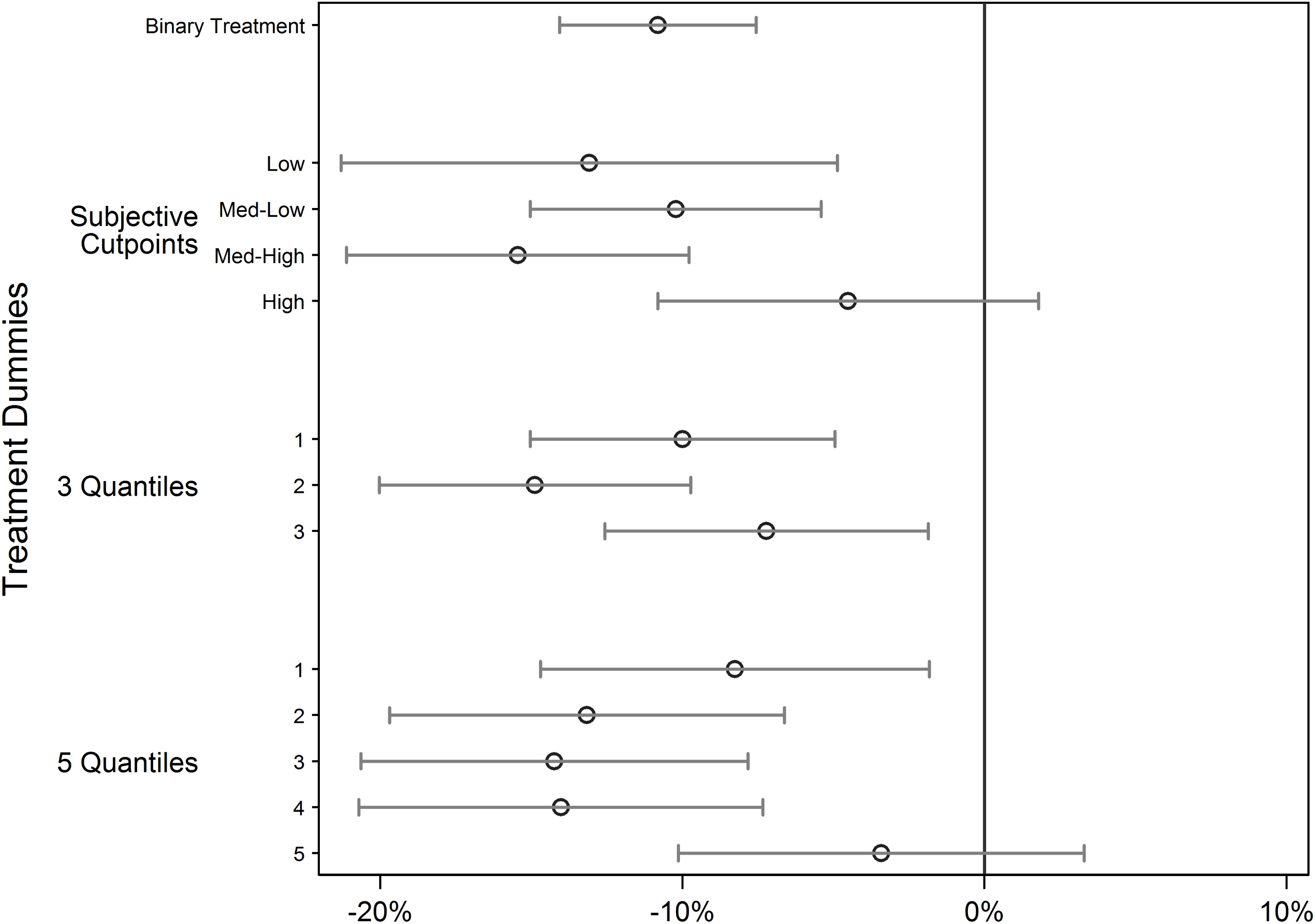
In the aggregate, we find a large negative effect,
![]() $-10.8$
percentage points averaged across all flooded counties. When we split the treatment group by treatment intensity, we find strong negative effects among the lightly and moderately flooded counties. As flood severity increases to the highest levels, the treatment effect is diminished somewhat, and disappears in some cases. Our preferred model for judging treatment effect heterogeneity, which uses subjective cutpoints, is instructive: we estimate that the flood cost Hoover 13.1%, 10.2%, and 15.5% of the two-party vote share in counties with low, medium-low, and medium-high levels of flooding and subsequent relief spending, constituting approximately three-quarters of flooded counties in the sample. However, in the most heavily hit counties, where 50% or more of the population was impacted, we cannot distinguish the flood’s effect from the null. Similar results are obtained when we use “objective” approaches to binning treated units, as shown in Figure 3.
$-10.8$
percentage points averaged across all flooded counties. When we split the treatment group by treatment intensity, we find strong negative effects among the lightly and moderately flooded counties. As flood severity increases to the highest levels, the treatment effect is diminished somewhat, and disappears in some cases. Our preferred model for judging treatment effect heterogeneity, which uses subjective cutpoints, is instructive: we estimate that the flood cost Hoover 13.1%, 10.2%, and 15.5% of the two-party vote share in counties with low, medium-low, and medium-high levels of flooding and subsequent relief spending, constituting approximately three-quarters of flooded counties in the sample. However, in the most heavily hit counties, where 50% or more of the population was impacted, we cannot distinguish the flood’s effect from the null. Similar results are obtained when we use “objective” approaches to binning treated units, as shown in Figure 3.

Figure 3. Effect estimates of flooding on Republican two-party vote share using different categories of flood severity. Coefficients and 95% confidence intervals are reported from linear models (
![]() $n=980$
). Categorizations include a binary treatment (top), subjective cutpoints in severity (0.1%–5%; 5%–20%; 20%–50%; and 50% and up) and objective cutpoints based on quantiles.
$n=980$
). Categorizations include a binary treatment (top), subjective cutpoints in severity (0.1%–5%; 5%–20%; 20%–50%; and 50% and up) and objective cutpoints based on quantiles.

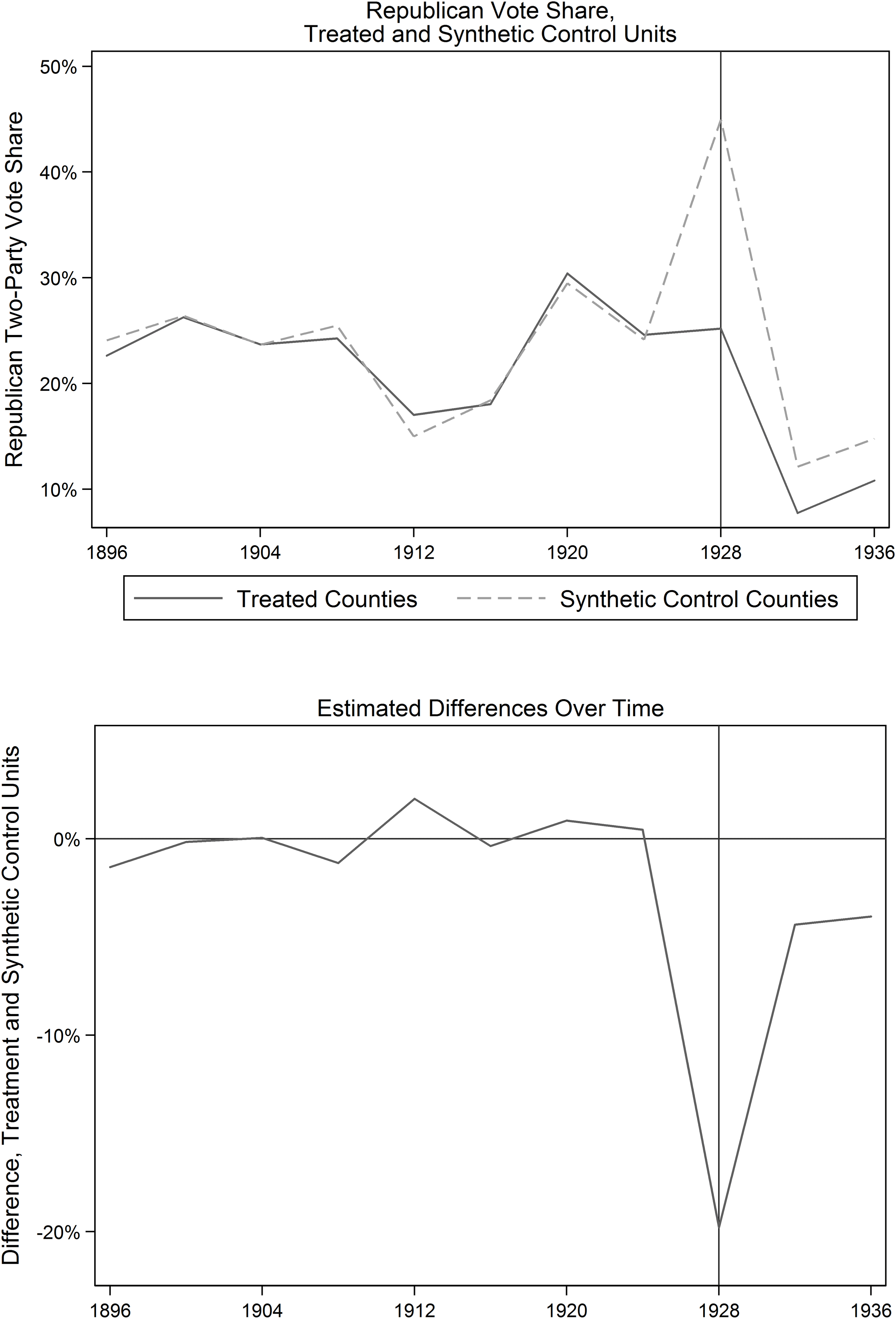
Figure 4. Estimate of the flood’s effect using a synthetic control model. The gap between treated counties (
![]() $n=95$
) and their synthetic control units, from 1896 to 1936. Treatment occurred prior to the 1928 election. The gap in 1928, our estimate of the SATT, is
$n=95$
) and their synthetic control units, from 1896 to 1936. Treatment occurred prior to the 1928 election. The gap in 1928, our estimate of the SATT, is
![]() $-$
19.8 percentage points.
$-$
19.8 percentage points.
The models reported in Figure 3 mimic standard approaches in the literature but rely on the so-called “parallel trends” assumption. Time-varying heterogeneity between treated and control units, if it exists, can bias our treatment effect estimates. Our treatment and control groups are substantially different in terms of their black and Protestant populations: counties in the treatment group have a mean black population of 44.5% and a mean Protestant population of 27.9%; the control group means in our southern sample are 26.8% and 37.2%, respectively. Although difference-in-differences models account for time-invariant heterogeneity, they do not account for heterogeneity that has disparate impact on outcomes across time. Both observed differences could produce bias toward a negative estimate that is specific to the 1928 election.Footnote 13
While the regression models we estimate control explicitly for both of these factors, we address lingering concerns over such heterogeneity using the synthetic control method (Abadie et al.
Reference Abadie, Diamond and Hainmueller2010). We employ this approach as a type of preprocessing, analogous to matching (Ho et al.
Reference Ho, Imai, King and Stuart2007), in an effort to account for both time-invariant and time-varying heterogeneity. For each treated county
![]() $i$
in the data, we follow a two-step approach: first, we select the donor pool of control counties that will be used in the synthetic control unit. We limit the donor pool to the 100 counties most closely matched to county
$i$
in the data, we follow a two-step approach: first, we select the donor pool of control counties that will be used in the synthetic control unit. We limit the donor pool to the 100 counties most closely matched to county
![]() $i$
in terms of pretreatment vote share.Footnote
14
Using this trimmed donor pool, we construct a synthetic control unit which most closely matches county
$i$
in terms of pretreatment vote share.Footnote
14
Using this trimmed donor pool, we construct a synthetic control unit which most closely matches county
![]() $i$
in terms of pretreatment vote share over the period 1896–1924.
$i$
in terms of pretreatment vote share over the period 1896–1924.
Under assumptions regarding match quality between a treated unit,
![]() $Y_{it}^{I}$
, and its synthetic control unit,
$Y_{it}^{I}$
, and its synthetic control unit,
![]() $\sum _{j=1}^{100}w_{j}Y_{jt}$
(where
$\sum _{j=1}^{100}w_{j}Y_{jt}$
(where
![]() $w$
is a vector of weights on the unit interval and
$w$
is a vector of weights on the unit interval and
![]() $Y_{jt}$
is a vector of control units comprising the donor pool), the difference in outcomes in 1928 represents an unbiased unit-specific treatment effect (Abadie et al.
Reference Abadie, Diamond and Hainmueller2010). Our estimand is the Sample Average Treatment Effect on the Treated (SATT), the mean of unit-specific treatment effects across 95 treated counties in the south.
$Y_{jt}$
is a vector of control units comprising the donor pool), the difference in outcomes in 1928 represents an unbiased unit-specific treatment effect (Abadie et al.
Reference Abadie, Diamond and Hainmueller2010). Our estimand is the Sample Average Treatment Effect on the Treated (SATT), the mean of unit-specific treatment effects across 95 treated counties in the south.
Figure 4 summarizes our results and illustrates the causal effect of the Mississippi Flood among southern counties affected by the flood. The top panel plots Republican two-party vote share for treatment and control groups from 1896 to 1936, while the bottom panel plots the mean difference in vote share between the two groups over the same period. Our approach yields high-quality matches on average over the period 1896 to 1924, before a precipitous drop in support for Hoover among flooded counties. The estimated difference in vote share in 1928 is
![]() $-$
19.8 percentage points, reducing Hoover’s vote share in flooded counties from 45% under the counterfactual to a mere 25.2% in reality. Unlike in the regression models reported previously, we do not observe meaningful treatment effect heterogeneity—our estimates range from a high of
$-$
19.8 percentage points, reducing Hoover’s vote share in flooded counties from 45% under the counterfactual to a mere 25.2% in reality. Unlike in the regression models reported previously, we do not observe meaningful treatment effect heterogeneity—our estimates range from a high of
![]() $-$
16.1 to a low of
$-$
16.1 to a low of
![]() $-$
24.2% across treatment levels and small changes across treatment levels are nonmonotonic. Treated counties at all levels of flood severity appear to have punished Hoover at the ballot box.
$-$
24.2% across treatment levels and small changes across treatment levels are nonmonotonic. Treated counties at all levels of flood severity appear to have punished Hoover at the ballot box.
5 Conclusion
Do voters punish incumbents indiscriminately for misfortune caused by natural disasters? Or do voters rationally evaluate the quality of relief efforts? Several recent studies cast doubt on the theory of blind retrospection, favoring a view of the electorate as “attentive”. But findings of voter attentiveness in the context of natural disasters have been drawn exclusively from cases in the post-New Deal era, while citizens’ expectations of government action have arguably expanded in line with the expansion of the state. To the extent that voters judge leaders’ performance relative to prevailing expectations, we expect reactions to natural disasters and subsequent relief efforts to vary across time and space.
We address external validity across time by studying the net effect of disaster and disaster relief in the case of the 1927 Mississippi Flood. Our analysis suggests that the effects of the flood on the 1928 presidential election were substantial and negative: we estimate that the flood cost Hoover 10.8 percentage points of the two-party vote share in affected counties. This estimate is not an artifact of modeling choice: in specifications that account for heterogeneity between treatment and control groups, our estimates of the flood’s effect increase further. Nor is it a function of sample selection: as we show in the Supplemental Appendix, our results are robust across a nationwide sample that includes an additional 35 flooded counties outside the South. This result is particularly surprising, given how extensive these relief efforts were at the time, and how closely associated Hoover himself was to the operation. The results seem to confirm concerns about external validity based on the context in which governments operate.
These findings generally support Achen and Bartels’ idea of blind retrospection, as the 1927 flood represents a hard case for the theory. But our results do not provide a full endorsement. While the net effect of the flood was broadly negative, we do not find that voters in harder-hit counties punished Hoover more. If anything, voters in counties that experienced less damage were more likely to punish Hoover—a distinction that runs counter to expectations of blind retrospection. Combined, our results raise two questions about retrospection in the wake of natural disasters—and the mechanisms by which it operates—that should guide future research. First, how does the extent to which voters are affected by a natural disaster shape their electoral behavior? Second, how do voters’ expectations of government response affect their vote choice in the wake of a disaster? By engaging these questions, scholars may be able to better understand the logic—or lack thereof—behind voters’ response to disaster and relief.
Supplementary material
For supplementary material accompanying this paper, please visit https://doi.org/10.1017/pan.2017.7.


