


Impact Statement
To devise efficient adaptation policies, it is key to understand the causes of past climate changes. Here, we present a method based on neural networks to estimate the past global mean surface temperature (GMST) anomalies caused by the changes in the greenhouse gas concentration, the variation of anthropogenic aerosols, and the variation driven by naturally occurring phenomena. This method is based on the training of a convolutional neural network using the estimations from 12 state-of-the-art climate models. Then we infer the most likely causes for the observed GMST changes from 1900 to 2014. The methodology presented could be applied in future studies to other variables or at the regional scale.
1. Introduction
Detection and attribution of climate change are key to understanding past climate change and devising adaptation policies. Detection aims to prove the existence of climate change exceeding its internal variability. Internal variability refers to climate variations resulting from processes intrinsic to the climate system. For instance, the global mean surface temperature (GMST) varies by a few tenths of degrees during the phases of the El Niño Southern Oscillation. Similarly, the Atlantic multidecadal variability can also influence the global climate. Boundary conditions of the climate system, known as forcings, can also cause climate change. The dominant forcings in the historical period (i.e., from 1850 to present day) are the increase in the greenhouse gases atmospheric concentration, the variations of the atmospheric aerosol concentration, the variations of solar insolation, the changes in land use, and stratospheric ozone concentrations. Anthropologically driven and naturally occurring forcings are generally considered separately. Attribution then aims to explain and quantify the impacts of the different forcings in the detected change, using both observations and climate models (Stott et al., Reference Stott, Gillet, Hegerl, Karoly, Stone, Zhang and Zwiers2010).
Hasselmann (Reference Hasselmann1993) defined a method to estimate the fingerprints of forced climate change based on the analysis of observation and the climate models. In the reference methods, such fingerprints are used to characterize the climate. The observations are linearly regressed onto the simulated responses of the external forcings using these fingerprints (Ribes et al., Reference Ribes, Planton and Terray2013). It is often assumed that the impacts of the forcings are additive. Detection and attribution studies often consider reduced dimensional data, using global spatial and temporal means. By doing so, they estimate a pseudo-invertible covariance matrix used for the linear regression (Zhang et al., Reference Zhang, Zwiers, Hegerl, Lambert, Gillett, Solomon, Stott and Nozawa2007). These methods have shown that global warming cannot be explained only by internal variability, and it was extremely likely that human activities had caused at least more than half of the observed increase in GMST from 1951 to 2010 (Gulev et al., Reference Gulev and Dentener2021).
State-of-the-art attribution methods have several limitations such as the additivity assumption of the influence of forcings, and attribute anomalies to more than two forcings are often difficult (Gillett et al., Reference Gillett, Kirchmeier-Young, Ribes, Shiogama, Hegerl, Knutti, Gastineau, John, Li and Nazarenko2021). We aim at exploring an alternative framework based on non-linear predictors to account for more complex interactions between the forcings. We then consider neural network regressors that have shown their ability to exploit spatial and temporal data structures, find patterns, and fuse heterogeneous sources of information efficiently in different domains of earth system sciences (Reichstein et al., Reference Reichstein, Camps-Valls, Stevens, Jung, Denzler and Carvalhais2019). We use convolutional neural networks (CNNs) and a variational inversion method, to perform climate change attribution. This accounts for the non-additivity in the forcings and is used to quantify the uncertainties in the attributed changes. Section 2 presents the data and the methodology. Section 3 is devoted to the results and Section 4 to the conclusions.
2. Data and Methods
2.1. Data
We use monthly air temperature from 1850 to 2014, from climate model simulations and observations. We use the outputs of the CMIP6 (Coupled Model Intercomparison Project 6; Eyring et al., Reference Eyring, Bony, Meehl, Senior, Stevens, Stouffer and Taylor2016) simulations performed with 12 ocean–atmosphere general circulation models (see Table 1 for details). We denote HIST as the historical simulations, using as varying boundary conditions all the external forcings. These forcings include the estimations of greenhouse gases, aerosols, ozone concentration, and the estimated past variation of solar activity and land use. Each climate model provides several simulation instances called members generated through a macro-perturbation of the initial conditions. We also use single-forcing simulations from the DAMIP (Gillett et al., Reference Gillett, Shiogama, Funke, Hegerl, Knutti, Matthes, Santer, Stone and Tebaldi2016) panel of CMIP6. These simulations used as varying boundary conditions only one of the external forcings, all the other external forcings being fixed at their value from 1850. We use the single-forcing simulations hist-aer denoted AER, hist-nat denoted NAT, and hist-GHG denoted GHG. They respectively use as varying forcing the anthropogenic aerosols, natural forcing (i.e., volcanic aerosol and solar variations), and greenhouse gases concentration. The effects of stratospheric ozone and land use were not investigated.
Table 1. Model and simulation used in this study.

Note. The numbers in the columns GHG, AER, and NAT provide the number of members used.
We also use observations (denoted OBS) of the 2 m air temperature over the continent from HadCRUT4 (Morice et al., Reference Morice, Kennedy, Rayner and Jones2012) blended with sea surface temperature from HadISST4 (Rayner et al., Reference Rayner, Parker, Horton, Folland, Alexander, Rowell, Kent and Kaplan2003). To make HIST and OBS comparable, we correct OBS of its blending effects using a 1.06 multiplier coefficient (Richardson et al., Reference Richardson, Cowtan and Millar2018). The missing values have been filled by kriging (Cowtan and Way, Reference Cowtan and Way2014).
All monthly data are converted into an annual mean and averaged spatially from 90
 $ {}^{\circ } $
S to 90
$ {}^{\circ } $
S to 90
 $ {}^{\circ } $
N. We then estimate the temperature anomalies in the 1900–2014 period (115 years). In each simulation (HIST, GHG, NAT, AER) we compute the mean temperature during the 1850–1900 period and remove it from the temperature. For the GISS-E2-1-G, we compute the temperature anomalies separately for the simulations using two different physics, with different schemes to calculate the aerosols indirect impact (Kelley et al., Reference Kelley, Schmidt, Nazarenko, Bauer, Ruedy, Russell, Ackerman, Aleinov, Bauer, Bleck, Canuto, Cesana, Cheng, Clune, Cook, Cruz, Del Genio, Elsaesser, Faluvegi, Kiang, Kim, Lacis, Leboissetier, LeGrande, Lo, Marshall, Matthews, McDermid, Mezuman, Miller, Murray, Oinas, Orbe, García-Pando, Perlwitz, Puma, Rind, Romanou, Shindell, Sun, Tausnev, Tsigaridis, Tselioudis, Weng, Wu and Yao2020). The same procedure is applied to OBS. Then, the time series of 115 years are normalized: for each model, we compute the maximum value of the ensemble mean of HIST and divide all the members of all simulation by this maximum. We also divide OBS by its maximum value.
$ {}^{\circ } $
N. We then estimate the temperature anomalies in the 1900–2014 period (115 years). In each simulation (HIST, GHG, NAT, AER) we compute the mean temperature during the 1850–1900 period and remove it from the temperature. For the GISS-E2-1-G, we compute the temperature anomalies separately for the simulations using two different physics, with different schemes to calculate the aerosols indirect impact (Kelley et al., Reference Kelley, Schmidt, Nazarenko, Bauer, Ruedy, Russell, Ackerman, Aleinov, Bauer, Bleck, Canuto, Cesana, Cheng, Clune, Cook, Cruz, Del Genio, Elsaesser, Faluvegi, Kiang, Kim, Lacis, Leboissetier, LeGrande, Lo, Marshall, Matthews, McDermid, Mezuman, Miller, Murray, Oinas, Orbe, García-Pando, Perlwitz, Puma, Rind, Romanou, Shindell, Sun, Tausnev, Tsigaridis, Tselioudis, Weng, Wu and Yao2020). The same procedure is applied to OBS. Then, the time series of 115 years are normalized: for each model, we compute the maximum value of the ensemble mean of HIST and divide all the members of all simulation by this maximum. We also divide OBS by its maximum value.
2.2. Methodology
First, we determine the relationship linking the GMST of HIST to that of GHG, AER, and NAT. We train a CNN using the time series of AER, GHG, and NAT as input, with a size of (3,115), and HIST as the target, with a size of (1,115). The resulting CNN estimates the GMST anomaly in the historical period from GHG, AER, and NAT GMST time series.
The CNN consists of 3 one-dimensional convolutional layers. The kernel size for all layers is 11, the input is zero-padded by 5 pixels, and the length of the layers is 10 in the CNN. Hyperbolic tangent is used as an activation function in the hidden layers to add non-linearities. The training phase is made of three steps using the mean square error (MSE): (a) we randomly select a climate model, (b) we randomly select an instance of each simulation (GHG, AER, NAT, and HIST), and (c) we train the network using the corresponding (GHG, AER, NAT) and HIST time series as input and target with a batch size of 100. We iterate this process
 $ 5\times {10}^6 $
times in total separated into 100 epochs of
$ 5\times {10}^6 $
times in total separated into 100 epochs of
 $ 5\times {10}^4 $
iterations. The procedure ensures that each model is used equally when training the CNN. The architecture and hyperparameters are chosen using a k-fold cross-validation technique. We considered the 12 models separately, leaving out the data of one climate model. We then train a CNN using the remaining 11 models and use the data from the excluded model as the validation set. The process is iterated by removing each model alternately and the mean validation error is estimated. The selected architecture provides the lowest mean validation error after varying the number of layers, the kernels sizes, and the lengths of the layers. The CNN is finally trained using the 12 models together.
$ 5\times {10}^4 $
iterations. The procedure ensures that each model is used equally when training the CNN. The architecture and hyperparameters are chosen using a k-fold cross-validation technique. We considered the 12 models separately, leaving out the data of one climate model. We then train a CNN using the remaining 11 models and use the data from the excluded model as the validation set. The process is iterated by removing each model alternately and the mean validation error is estimated. The selected architecture provides the lowest mean validation error after varying the number of layers, the kernels sizes, and the lengths of the layers. The CNN is finally trained using the 12 models together.
2.2.1. Variational inversion
The detection attribution problem aims at estimating the input time series (GHG, AER, and NAT) corresponding to the OBS time series. Therefore, we use a variational approach and the trained CNNs estimating the contribution of each forcing in the multi-model dataset. In geophysics, the variational inversion (Diouf et al., Reference Diouf, Thiria, Niang, Brajard and Crépon2011; Brajard et al., Reference Brajard, Santer, Crépon and Thiria2012) considers a physical phenomenon and an associated model M. The variational inversion seeks to infer the physical parameters that led to the observations, according to the geophysical model. It often implies the use of the adjoint model of M which estimates changes in the input in response to a disturbance of the output values calculated by M. The basic idea is to determine the minimum of a cost function J that measures the disagreements between the observations and the model estimations. Due to the complexity of the model, the desired minimum is classically obtained by using gradient methods, to estimate the control parameters. In our case, we use the CNN as a model M so this process is straightforward and the inversion is obtained using the classical backpropagation algorithm. In our case, the parameters we are looking for are the input of the CNN with OBS at output. The inversion is an “ill-posed” problem that has multiple solutions and needs the estimation of the parameter distribution; moreover, the method is sensitive to the initialization. To overcome these (Bauer et al., Reference Bauer, Tsigaridis, Faluvegi, Kelley, Lo, Miller, Nazarenko, Schmidt and Wu2020) problems, we repeat the process using different starting points. We use as a cost function the MSE and add a penalization term. This penalization is needed to keep a physically coherent solution. The cost function is
 $$ J(X)\hskip0.35em =\hskip0.35em MSE\left( OBS, CNN(X)\right)+B\times MSE\left(X, Xst\right) $$
where B is a scaling factor, set to 0.01, Xst the initial value of the inputs, and X input to be determined. This minimization is iterated until
 $ MSE\left( OBS, CNN(X)\right) $
is less than 0.05
$ MSE\left( OBS, CNN(X)\right) $
is less than 0.05
 $ {}^{\circ } $
C/
$ {}^{\circ } $
C/
 $ {}^{\circ } $
C. To choose the initial value Xst, we used multiple physically consistent values. For each of the 12 climate models, we randomly select 100 triplets of members of GHG, AER, and NAT for Xst and generate 1,200 variational inversions.
$ {}^{\circ } $
C. To choose the initial value Xst, we used multiple physically consistent values. For each of the 12 climate models, we randomly select 100 triplets of members of GHG, AER, and NAT for Xst and generate 1,200 variational inversions.
3. Results
3.1. Neural network performance
We evaluate the ability of the proposed approach to estimate the GMST from the HIST simulations using the k-fold cross-validation. For each climate model, we use a CNN trained with the data excluding that model using the 11 other climate models. Table 2 presents the training (validation) root mean square error (RMSE) in the first column (second column) when the CNN has seen the outputs (or not seen the outputs) from the climate model. All the RMSE is provided here for the normalized time series so that the unit is
 $ {}^{\circ } $
C per
$ {}^{\circ } $
C per
 $ {}^{\circ } $
C. We obtain a mean training RMSE of 0.15
$ {}^{\circ } $
C. We obtain a mean training RMSE of 0.15
 $ {}^{\circ } $
C/
$ {}^{\circ } $
C/
 $ {}^{\circ } $
C and a validation RMSE of 0.17
$ {}^{\circ } $
C and a validation RMSE of 0.17
 $ {}^{\circ } $
C/
$ {}^{\circ } $
C/
 $ {}^{\circ } $
C across the climate models. The training RMSE is only slightly lower than the validation RMSE so that the CNN avoids overfitting. The RMSE varies among the models, with values from 0.09
$ {}^{\circ } $
C across the climate models. The training RMSE is only slightly lower than the validation RMSE so that the CNN avoids overfitting. The RMSE varies among the models, with values from 0.09
 $ {}^{\circ } $
C/
$ {}^{\circ } $
C/
 $ {}^{\circ } $
C (0.1
$ {}^{\circ } $
C (0.1
 $ {}^{\circ } $
C/
$ {}^{\circ } $
C/
 $ {}^{\circ } $
C) in CanESM5 to 0.20
$ {}^{\circ } $
C) in CanESM5 to 0.20
 $ {}^{\circ } $
C/
$ {}^{\circ } $
C/
 $ {}^{\circ } $
C (0.24
$ {}^{\circ } $
C (0.24
 $ {}^{\circ } $
C/
$ {}^{\circ } $
C/
 $ {}^{\circ } $
C) in NorESM1-LM for the training (validation) RMSE. The reason for these differences remains to be fully investigated, but we suggest that the output of the CNN reflects the similarities among models, and a low performance reflects a singularity of the GMST simulated by one model. We verify that the validation performance of a simple baseline linear network consisting of only a linear layer has a larger mean validation error of 0.21
$ {}^{\circ } $
C) in NorESM1-LM for the training (validation) RMSE. The reason for these differences remains to be fully investigated, but we suggest that the output of the CNN reflects the similarities among models, and a low performance reflects a singularity of the GMST simulated by one model. We verify that the validation performance of a simple baseline linear network consisting of only a linear layer has a larger mean validation error of 0.21
 $ {}^{\circ } $
C/
$ {}^{\circ } $
C/
 $ {}^{\circ } $
C so that non-linearities do improve the performance.
$ {}^{\circ } $
C so that non-linearities do improve the performance.
Table 2. (First column) Training RMSE (
 $ {}^{\circ } $
C/
$ {}^{\circ } $
C/
 $ {}^{\circ } $
C) computed on the outputs of the climate model when that model is seen by the CNN; (Second column) Validation RMSE (
$ {}^{\circ } $
C) computed on the outputs of the climate model when that model is seen by the CNN; (Second column) Validation RMSE (
 $ {}^{\circ } $
C/
$ {}^{\circ } $
C/
 $ {}^{\circ } $
C) computed on the outputs of the climate model when the model is not seen by the CNN.
$ {}^{\circ } $
C) computed on the outputs of the climate model when the model is not seen by the CNN.
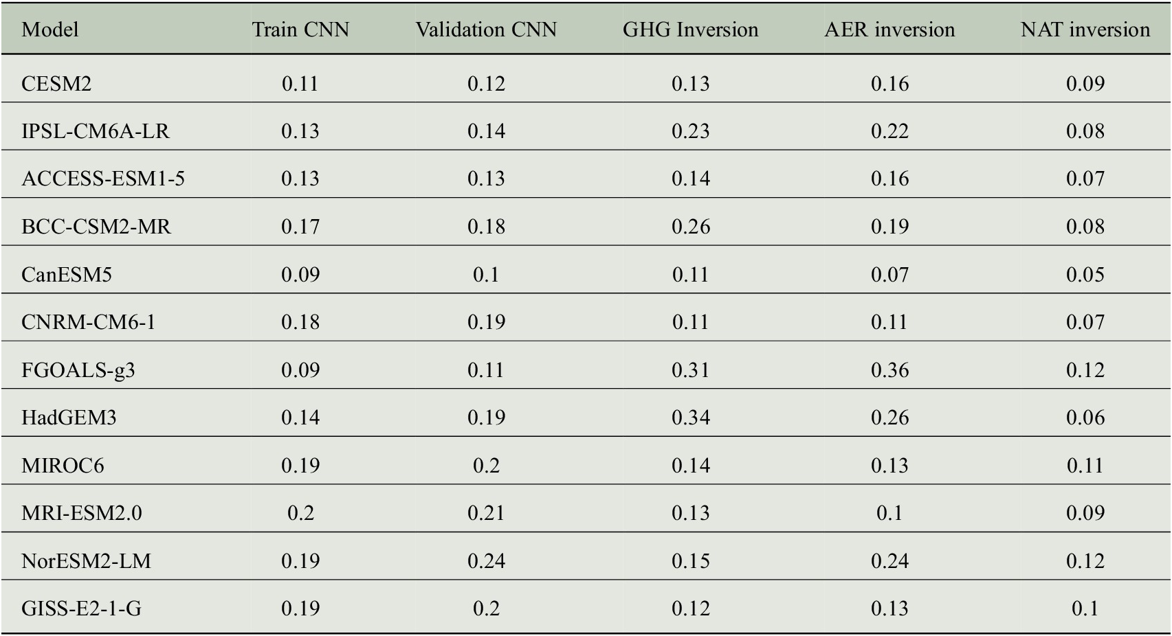
Note. (Last three columns) Mean RMSE (
 $ {}^{\circ } $
C) between the mean inversion of the effects of greenhouse gases (anthropogenic aerosols and natural forcings) and the GMST from the ensemble mean of GHG (AER and NAT).
$ {}^{\circ } $
C) between the mean inversion of the effects of greenhouse gases (anthropogenic aerosols and natural forcings) and the GMST from the ensemble mean of GHG (AER and NAT).
3.2. Variational inversion
To validate the variational inversion, we used the members of HIST as pseudo-observations and the k-fold framework. For each HIST members for each climate models, we produce the variational inversions with 100 randomly chosen starting points using the CNN trained from data excluding that climate model. Then, the inversions are denormalized. As an illustration, one HIST instance was chosen randomly and is shown in Figure 1, black line. The mean inversion with the forcing of greenhouse gases, anthropogenic aerosols, and natural forcings (Figure 1, red, blue, and green lines) is then compared to the ensemble mean GMST of GHG, AER, and NAT (Figure 1, purple, dark blue and beige lines in Figure 1). The color shades in Figure 1 quantify the spread among the inversions found from the different starting points, with one standard deviation. The spread of the simulations GHG, AER, and NAT illustrates one standard deviation across the available ensemble members. The greenhouse gases influence is variable among models, as the inversion results simulate in 2014 a GMST varying from 1
 $ {}^{\circ } $
C to 2
$ {}^{\circ } $
C to 2
 $ {}^{\circ } $
C. This reflects the different sensitivity of climate models. The result of the anthropogenic aerosols inversion also scale with the climate sensitivity, with a large cooling for sensitive models. Nevertheless, FGOALs-g3, IPSL-CM6A-LR, or BCC-CSM2-MR simulate weak anomalies for anthropogenic aerosols compared to AER but large anomalies for greenhouse gases. Conversely, HadGEM3 or NorESM2-LM simulates rather large anomalies for anthropogenic aerosols and for HadGEM3 rather weak anomalies for greenhouse gases. The inversions provide realistic values for the natural forcings that agree with the outputs from NAT, with time series with small anomalies, except for the cooling in 1963, 1982, and 1991, following the major eruptions of Agung, El Chichon, and Pinatubo. For all models, the inversions have a large spread, much larger than the spread of the simulations GHG, AER, or NAT. It reflects the diversity of starting points used in the inversions. In 7 out of 12 models, we found a good agreement between the inversions and the simulated anomalies forcings as the spread of inversions agrees with the mean simulated anomalies. However, for FGOALs-g3, BCC-CSM2-MR, HadGEM3, NorESM2-LM, IPSL-CM6A-LR, the inversion is biased.
$ {}^{\circ } $
C. This reflects the different sensitivity of climate models. The result of the anthropogenic aerosols inversion also scale with the climate sensitivity, with a large cooling for sensitive models. Nevertheless, FGOALs-g3, IPSL-CM6A-LR, or BCC-CSM2-MR simulate weak anomalies for anthropogenic aerosols compared to AER but large anomalies for greenhouse gases. Conversely, HadGEM3 or NorESM2-LM simulates rather large anomalies for anthropogenic aerosols and for HadGEM3 rather weak anomalies for greenhouse gases. The inversions provide realistic values for the natural forcings that agree with the outputs from NAT, with time series with small anomalies, except for the cooling in 1963, 1982, and 1991, following the major eruptions of Agung, El Chichon, and Pinatubo. For all models, the inversions have a large spread, much larger than the spread of the simulations GHG, AER, or NAT. It reflects the diversity of starting points used in the inversions. In 7 out of 12 models, we found a good agreement between the inversions and the simulated anomalies forcings as the spread of inversions agrees with the mean simulated anomalies. However, for FGOALs-g3, BCC-CSM2-MR, HadGEM3, NorESM2-LM, IPSL-CM6A-LR, the inversion is biased.

Figure 1. GMST for an HIST member (black) randomly chosen as pseudo-observation, the mean results of variational inversions from the same member for the (red) greenhouse gases, (blue) anthropogenic aerosols and (green) natural forcings effects and ensemble mean of the (purple) GHG, (dark blue) AER and (beige) NAT. The color shades show one standard deviation across the inversion or across the ensemble members.
The mean RMSEs between the mean inversions results of each HIST instance and the ensemble mean of the corresponding single-forcing simulation are presented in Table 2. RMSEs for BCC-CSM2-MR, IPSL-CM6A-LR, HadGEM3, and FGOALS-g3 RMSEs are large for the influence of greenhouse gases with, respectively, 0.26, 0.23, 0.34, and 0.31
 $ {}^{\circ } $
C. Similarly, the influence of anthropogenic aerosols is not well retrieved for FGOALS-g3 (RMSE of 0.36
$ {}^{\circ } $
C. Similarly, the influence of anthropogenic aerosols is not well retrieved for FGOALS-g3 (RMSE of 0.36
 $ {}^{\circ } $
C), HadGEM3 (0.26
$ {}^{\circ } $
C), HadGEM3 (0.26
 $ {}^{\circ } $
C) and NorESM2-LM (0.24
$ {}^{\circ } $
C) and NorESM2-LM (0.24
 $ {}^{\circ } $
C), and IPSL-CM6A-LR (0.22
$ {}^{\circ } $
C), and IPSL-CM6A-LR (0.22
 $ {}^{\circ } $
C). This confirms the analysis of Figure 1, where these models all simulate contrasted GMST in the results of anthropogenic aerosols and greenhouse gases inversion results.
$ {}^{\circ } $
C). This confirms the analysis of Figure 1, where these models all simulate contrasted GMST in the results of anthropogenic aerosols and greenhouse gases inversion results.
The validation RMSEs reflect the distance of the climate models from the multi-model average. This distance results from the different climate sensitivity in each model, as well as the implementation of anthropogenic aerosol forcing, which varies between models (Pincus et al., Reference Pincus, Forster and Stevens2016).
To attribute the observed changes, we apply the variational inversion to the observed GMST. The starting points provide 1,200 results of the effects of the greenhouse gases (Figure 2, red line), anthropogenic aerosol (Figure 2, blue line), and natural forcing (Figure 2, green line). The spread is evaluated using the standard deviation across the inversions (shades in Figure 2, left panel). The greenhouse gases and anthropogenic aerosols influence is smaller compared to many of the models illustrated in Figure 1, with variations consistent with that simulated in GHG and AER. The effect of natural forcings remains small compared to the results of Figure 1, with only a small decrease in the GMST in 1992 and 1993 following the Pinatubo eruption. The right panel Figure 2 illustrates the distribution of the results from the inversions in 1993 and 2014. We study in particular the year 1993 following the 1991 Pinatubo eruption and 2014 as it is the last year of the time series. The distribution shows a large spread for the effects of forcings associated with the diversity of the starting points used. When using the 95 percent intervals from the distribution of the inversion, the results show a range of [0.8
 $ {}^{\circ } $
C,1.9
$ {}^{\circ } $
C,1.9
 $ {}^{\circ } $
C] for greenhouse gases, [−0.7
$ {}^{\circ } $
C] for greenhouse gases, [−0.7
 $ {}^{\circ } $
C,-0.1
$ {}^{\circ } $
C,-0.1
 $ {}^{\circ } $
C] for anthropogenic aerosols, and [−0.1
$ {}^{\circ } $
C] for anthropogenic aerosols, and [−0.1
 $ {}^{\circ } $
C,0.3
$ {}^{\circ } $
C,0.3
 $ {}^{\circ } $
C] for natural forcings in 2014. In 1993, the effect of natural forcing is with a 95 percent intervals of [−0.5
$ {}^{\circ } $
C] for natural forcings in 2014. In 1993, the effect of natural forcing is with a 95 percent intervals of [−0.5
 $ {}^{\circ } $
C,0.1
$ {}^{\circ } $
C,0.1
 $ {}^{\circ } $
C] consistent with well-known effects of volcanic aerosols following the Pinatubo eruption (Gulev et al., Reference Gulev and Dentener2021). We can compare these results (Figure 2, right) to the results found in Gillett et al. (Reference Gillett, Kirchmeier-Young, Ribes, Shiogama, Hegerl, Knutti, Gastineau, John, Li and Nazarenko2021) using the same data but with the regularized optimal fingerprinting method. They found anomalies of [1.2
$ {}^{\circ } $
C] consistent with well-known effects of volcanic aerosols following the Pinatubo eruption (Gulev et al., Reference Gulev and Dentener2021). We can compare these results (Figure 2, right) to the results found in Gillett et al. (Reference Gillett, Kirchmeier-Young, Ribes, Shiogama, Hegerl, Knutti, Gastineau, John, Li and Nazarenko2021) using the same data but with the regularized optimal fingerprinting method. They found anomalies of [1.2
 $ {}^{\circ } $
C,1.9
$ {}^{\circ } $
C,1.9
 $ {}^{\circ } $
C] for greenhouse gases, [−0.7
$ {}^{\circ } $
C] for greenhouse gases, [−0.7
 $ {}^{\circ } $
C,-0.1
$ {}^{\circ } $
C,-0.1
 $ {}^{\circ } $
C] for anthropogenic aerosols, and [0.01
$ {}^{\circ } $
C] for anthropogenic aerosols, and [0.01
 $ {}^{\circ } $
C,0.06
$ {}^{\circ } $
C,0.06
 $ {}^{\circ } $
C] for natural forcings in the 2010–2019 decade. This suggests that the variational inversion provides coherent results values but with larger confidence intervals.
$ {}^{\circ } $
C] for natural forcings in the 2010–2019 decade. This suggests that the variational inversion provides coherent results values but with larger confidence intervals.
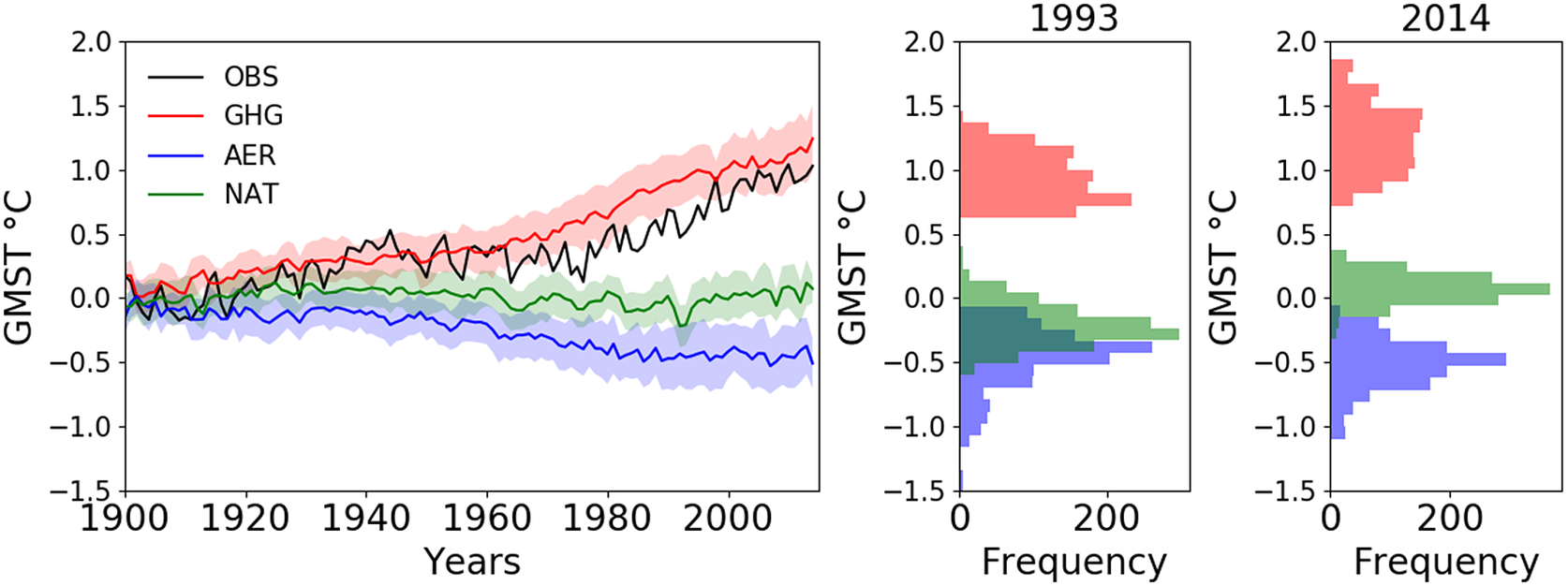
Figure 2. Left: (black) Observation in
 $ {}^{\circ } $
C and variational inversion for (red) greenhouse gases, (blue) anthropogenic aerosols, and (green) natural forcings. Shades show the standard deviation across the 1,200 varational inversion. (Right): Histogram from the inversion for (red) greenhouse gases,(blue) anthropogenic aerosols, and (green) natural forcings for the year 1993 and 2014.
$ {}^{\circ } $
C and variational inversion for (red) greenhouse gases, (blue) anthropogenic aerosols, and (green) natural forcings. Shades show the standard deviation across the 1,200 varational inversion. (Right): Histogram from the inversion for (red) greenhouse gases,(blue) anthropogenic aerosols, and (green) natural forcings for the year 1993 and 2014.
4. Conclusion
In this article, we proposed an original solution to the attribution problem that does not rely on the classical forcing additivity assumption. The estimation relies on a non-linear forcing combination model that is learned from climate models simulations using GMST as an example. Spatial information of data will be included in future works. We chose however to not use it in this study to compare our results to previous studies, using mostly the GMST. The results found are coherent with a previous study using the same dataset and a classic fingerprinting method (Gillett et al., Reference Gillett, Kirchmeier-Young, Ribes, Shiogama, Hegerl, Knutti, Gastineau, John, Li and Nazarenko2021) but with a larger uncertainty due in part to the different starting points of the inversion. For 4 of the 12 climate models, the validation score is lower. Other choices of architectures could be tested to combine more realistically the effects of forcings like recurrent neural networks more adapted to time series. Alternative variational inversion frameworks like other cost functions or starting points could also be tested. This new method could be applied in case a large non-additivity is expected in other variables (precipitation for example) or at the regional scale (Lehner and Coats, Reference Lehner and Coats2021).
Abbreviations
- AER
-
hist-aer simulations
- CMIP6
-
Coupled Model Intercomparison Project 6
- CNN
-
convolutionnal neural network
- GHG
-
hist-GHG simulations
- GMST
-
global mean surface temperature
- GSAT
-
global surface air temperature
- HIST
-
historical simulations
- MSE
-
mean square error
- NAT
-
hist-nat simulations
- OBS
-
observations
- RMSE
-
root mean square error
Acknowledgments
We are grateful for the technical assistance of Carlos Mejia, Alexandre Bône, and Michel Crépon. This work was performed using HPC ressources from GENCI-IDRIS (grant 2021-AD011013295).
Author Contributions
Conceptualization, methodology, and visualization: G.G, S.T., and C.B,; Software and formal analysis: C.B.; Writing: G.G., S.T., C.B., and P.G; Resources: G.G.; Investigation: C.B. and G.G; all authors approved the final submitted draft.
Competing Interests
The authors declare no competing interests exist.
Data Availability Statement
Data and codes can be found in https://gitlab.com/ConstantinBone/detection-and-attribution-of-climate-change-a-deep-learning-and-variational-approach.
Ethics Statement
The research meets all ethical guidelines, including adherence to the legal requirements of the study country.
Funding Statement
This research was supported by grants from the Sorbonne Center for Artificial Intelligence (SCAI). Part of this work has been supported by project ChairesIA 2019—DL4CLIM ANR-19-CHIA-0018-01. The funder had no role in study design, data collection and analysis, decision to publish, or preparation of the manuscript.
Provenance
This article is part of the Climate Informatics 2022 proceedings and was accepted in Environmental Data Science on the basis of the Climate Informatics peer review process.


 Open access