


1. Introduction
In order to give an answer to the important question of whether the big ice sheets of the world, in Greenland and the Antarctic, are decreasing, increasing or even in equilibrium, several attempts have been made to set up total mass balance equations. The debit side of these budgets contains two items, (a) Loss due to melting and evaporation (ablation), (b) Loss due to calving. Approximate values of the total loss and the loss due to calving per year for Greenland and Antarctica are shown in Table I. The values given in this table are attended with great uncertainty, but what can be deduced with certainty is that the loss due to calving constitutes a large part of the total loss (about 50 per cent for Greenland and about 90 per cent for Antarctica). Consequently, a necessary condition for finding a reliable mass balance for the big ice sheets is to obtain a rather accurate value of the loss of ice by calving.
Table I. Approximate Values of the Loss of Ice from the Greenland and Antarctic Ice Sheets

Seen in this context, the importance of throwing some light on the factors influencing the calving process is obvious. The considerations put forward in this paper are an attempt to do this.
2. Deformation and Stress in a Floating Glacier
In the following, the term “floating glacier” will be applied to the subject discussed, but it should be pointed out that floating ice shelves are also included.
Consider a portion of a floating glacier of constant thickness h (cf. Fig. 1). In order to keep an arbitrary proportion of the glacier in equilibrium in the sense that the rates of strain in all directions are equal to zero, the stress distribution must be purely hydrostatic, i.e. all shear stresses must be equal to zero, and all normal stresses equal to ρ i gy, where ρ i is the density of the ice (assumed constant), g the acceleration due to gravity, and y the vertical distance from the upper surface. At the front of the floating glacier (which for simplicity is assumed vertical) the normal stress is equal to the water pressure and distributed as shown in Figure 1, i.e. it varies linearly from zero at water level to the value ρ w gh′ = ρ i gh t the bottom surface. Comparing this stress distribution with that necessary for keeping the ice in equilibrium, it is seen that the actual stresses are insufficient to maintain equilibrium. The deviation between the hydrostatic pressure and the actual pressure is a tensile force N, and consequently the ice must expand in the direction of the tensile force, i.e. in the direction perpendicular to the front. This expansion has been considered by Reference WeertmanWeertman (1957).

Fig. 1. Longitudinal section of floating glacier
As will be seen from Figure 1, the deviation between the actual pressure and the hydrostatic pressure increases from the bottom to the top of the glacier, which means that the tensile force acts eccentrically. In other words, the floating glacier is subject to bending as well. Consequently, the upper layers will be stretched more than the lower layers, so that the front of the ice begins to rotate, overhanging more and more. This rotation cannot proceed without a simultaneous downward movement of the frontal part. This, in turn, causes upward-directed buoyancy forces to act on the front section of the glacier. If the front of the glacier is situated far from bedrock contact, then the necessary reaction to this upward-directed force must come from the neighbouring section of the glacier, which starts moving upwards for this reason. Applying this argument to consecutive sections of the floating glacier, it will he realised that in this way a series of undulations with their axes parallel to the ice front arc developed. The amplitude of the undulations decreases according to the distance from the ice front. This procedure takes place at the same time as the glacier is expanding. At some distance from the front the vertical deflection has in practice disappeared, and here the glacier is in a state of pure expansion. This is the state considered by Weertman, who also pointed out that his theory is valid only at some distance from the ice front.
The assumption that the ice front is situated far from bedrock contact is correct with regard to the big ice shelves of Antarctica. Elsewhere, the number of undulations developed depends on the distance between the front and the bedrock in the direction perpendicular to the ice front.
Now let us turn to the stress distribution in the glacier, proceeding with the descriptive account followed so far. A more precise treatment of the subject is given in section 3, where the theory is put in a mathematical form. It has already been stated that when stress deviation from hydrostatic pressure is considered, the glacier is subject to a tensile force acting on the front, and that the tensile stresses arc greatest at the upper surface of the glacier. As the frontal part moves downwards, transverse forces start acting on the glacier, inducing shear stresses in the ice body. In this way a rather complex state of stress is developed in the frontal part of the glacier.
As shown in section 4, the tensile stresses, as well as the shear stresses, reach their maximum at a cross-section situated at a distance from the front approximately equal to the thickness of the glacier. Since the combination of tensile stress and shear stress is very dangerous, from the point of view of fracture, it seems reasonable to assume that the mechanism described here will lead to fracture developing from the upper surface of the glacier, where the tensile stresses are greatest.
Several simplifications and inaccuracies have been made in the above considerations. The most important simplifications are discussed below.
The deviation between the hydrostatic pressure and the actual pressure acting at the front was claimed to be an eccentrically acting, tensile force. As the frontal part of the glacier moves downwards, however, the magnitude of the force, as well as the eccentricity, varies continuously. In fact, the force acting on the front becomes a compressive force from a certain moment, but an essential point is that the bending moment at the front increases slightly during the downward movement and, consequently, keeps the process going.
It was also assumed that the front was vertical. This is in practice the case as regards that part of the front above sea-level. According to Reference Swithinbank, Zumberge and HathertonSwithinbank and Zumberge (1965), p. 201 the shape of the front below sea-level may differ considerably from the vertical. Therefore, let us examine the effect of the front shapes shown in Figure 2. In addition to the normal force N, the action of which was considered above, the cross-section marked with the dotted line is now influenced also by a vertical force Q downward or upward, depending on whether the front is overhanging or not (Fig. 2a and b). This causes a movement of the frontal part in the direction of the force. By this movement, however, the force is decreased and, consequently, the glacier would approach a state of equilibrium in which the force had disappeared if the force Q were the only force acting on it. This shows that whatever the shape of the frontal part of the glacier, it will only modify, but not prevent, the deformation process previously described.

Fig. 2. Forces acting at the front of the glacier
3. Development of Basic Equations
3.1 General remarks
In this section the equations for the stresses and deformations of the floating glacier are set up. The theory developed is analogous to beam theory used for determining stresses and deflections of a beam of an elastic material. As is most frequently the case when dealing with a problem from nature, a correct treatment, if possible at all, will involve enormous mathematical troubles. In order to avoid these troubles a simplified system—a model—has to be introduced. Before describing the model adapted for the calculation, mention of the system proper would be appropriate.
We are dealing with a glacier which moves from land out into the sea (Fig. 3). At the point where the depth of the sea is equal to d i h, (d i = ρ i/ρ w) the frontal part of the glacier comes afloat. Observations, as well as theoretical considerations, indicate that the velocity is practically constant over the entire thickness of the glacier. If the extension of the glacier in the direction parallel to the front, i.e. normal to the plane of the paper (Fig. 3), is supposed large, the glacier may therefore with good approximation be regarded as moving into the sea as a rigid body. If the inclination of the ground over which the glacier moves is supposed slight, then the buoyancy forces resulting from the oblique, downward movement of the front into the sea, will be compensated by a simultaneous upward movement of the frontal part of the glacier (compare the remarks in connection with Figure 2, section 2). This means that, apart from the vertical deflections caused by the bending moment acting at the front, the glacier will move into the sea as a free-floating body. The extent of the floating part of the glacier increases in course of time, partly due to the supply of ice from the tributary of the glacier, which causes a translational movement, and partly due to the extension of the glacier itself owing to the tensile force mentioned in section 2.

Fig. 3. Longitudinal section of floating glacier
From time to time a piece of the frontal part of the glacier will break off, and in this way a state of equilibrium is attained in which the loss by calving balances the supply of ice from behind. If the supply of ice is supposed constant, the front of the glacier will fluctuate around a state of equilibrium.
The co-ordinate system used in the calculation forms part of the translational movement of the glacier. The velocity resulting from the extension of the glacier itself is neglected. Mathe-matically, this means that total derivatives
As shown by the calculations (see section 4), the position of the point of transition may vary considerably without influencing the deformation of the frontal part very much. For this reason, the point of transition is considered fixed, in relation to the co-ordinate system. This is tantamount to assuming the extent of the floating part of the glacier to be constant.
To sum up, the following approximations are made:
(a) The extent of the glacier in the direction parallel to the front is supposed large, i.e. we are dealing with the case of plane strain.
(b) Apart from the vertical deflections caused by the bending moment acting on the front, the glacier floats freely.
(c) The extent of the floating part of the glacier is assumed constant.
To these assumptions we add one more, viz.
(d) The thickness of the glacier is supposed constant. Actually, the thickness varies, duc to melting—possibly deposition of snow or ice—and also due to the extension creep which may cause thinning of the glacier.
3.2. The co-ordinate system
An x 1-axis is located at the middle surface of the undeflected glacier (parallel to sea-level), directed perpendicular to the ice front. The deviation of the middle surface of the glacier from the horizontal plane containing the x 1-axis is denoted u. The deflection u is positive in the upward direction. The x 2-direction is normal to the middle surface of the undeflected glacier with origin at the middle surface of the deflected glacier, and positive downwards (see Fig. 3).
3.3. Forces acting on a cross-section of the glacier
Consider a section of unit width in the direction normal to the plane of the paper. The stresses acting on a cross-section normal to the x 1-axis may be reduced to three forces, which can statically replace the stresses (see Fig. 4) viz.


Fig. 4. Forces acting on an element of the glacier
σ 11and σ 12 denote normal stress and shear stress, respectively. The sign-convention for forces and stresses will appear from Figure 4.
3.4. Equations of equilibrium
Since all movements are very slow, inertial forces may be neglected. Consequently, the equations of equilibrium used in statics can be applied. Neglecting the small contributions to the moment from the normal force and the horizontal component of the water pressure, the application of these equilibrium conditions to an element of the glacier leads to the well-known equations

and

In these equations q denotes the transverse load on the glacier, i.e.
Substituting Equation (6) into Equation (4) and introducing dimensionless variables

and

where L is the length of the floating part of the glacier, and the other symbols are as explained above, Equations (4) and (5) are rewritten


Differentiating Equation (8) once with respect to x′1 and substituting dQ′/dx′1 from Equation (7) leads to

The dimensionless normal force, obtained from an equilibrium condition, may be expressed by
3.5. Stress-strain relationship
So far, only statical conditions have been applied, which are independent of the rheological properties of the ice. In order to proceed further, the relationship between stress and strain for the ice must be considered. Ice is known to possess viscous as well as elastic properties. If, however, stress variations take place very slowly, as in the case here considered, the elastic terms occurring in the stress-strain relationship are negligible, and consequently ice may in this connection with good approximation be treated as a purely viscous material. Hence, applying the notation of Cartesian tensors the stress-strain relationship may he expressed by the equation

where
where θ is the temperature in degrees Celsius, and τ the effective shear stress defined by the equation:
where σ′ ij is the deviatoric stress
The effective shear stress varies considerably throughout the glacier. Moreover, the temperature varies in the vertical direction through the glacier. Evidence of such a variation is given for the Antarctic ice shelves (see Reference Bender and GowBender and Gow (1961)), for which the temperature difference between the upper and lower surfaces may amount to 20 deg or more. A similar temperature variation, perhaps not so marked, may be expected for the big ice streams of Greenland.
From these remarks, in conjunction with Equation (12), it follows that a correct treatment of the problem would require consideration of the great variation (by a factor ten or more) of the viscosity. This, however, would involve enormous mathematical troubles. Since a fundamentally correct solution may be obtained assuming the viscosity constant, and since the mathematical treatment is greatly facilitated by this assumption, the viscosity of the ice is supposed constant, although with this assumption the results obtained by the calculation (e.g. the width of the icebergs produced by calving or the time interval between two calvings) cannot be expected to agree with nature. On the other hand, the results will give an indication of the variation of these quantities with the mean temperature, density and thickness of the glacier.
3.6. Differential equation for the deflection curve
According to beam theory, the curvature of a beam of an elastic material having a narrow rectangular cross-section may to a first approximation be expressed by

where E is Young’s modulus of elasticity. Equation (14) is based on the assumption that plane cross-sections remain plane during the deformation.
Comparing the stress-strain relationships for the elastic material with that for the viscous material, it can be shown that the corresponding equation for an infinitely wide beam of a viscous material is expressed by

In this equation d/dt has been replaced by ∂/∂t in accordance with the remarks on p. 218.
In section 2 it was mentioned that only deviations of stress from the hydrostatic pressure will result in deformations. For this reason the moment forming part of the right-hand side of Equation (15) equals the moment of the stress deviation between the actual normal stresses and the hydrostatic pressure. Since the quantity previously denoted by M is the moment of the actual stresses, it may be realised that M in Equation (15) should be replaced with

Substituting this expression into Equation (15) and introducing dimensionless variables, this equation is rewritten
The dimensionless time is introduced as t′ = t/T, where T is a fixed time interval.
Differentiating Equation (16) twice with respect to x 1 and substituting


where c = ρ w ghT/μ is a dimensionless constant. Equation (17) is the differential equation for the deflection curve of the floating glacier, and is analogous with the differential equation for the deflection curve of a beam on an elastic foundation.
3.7. Boundary conditions
At the transition from the grounded part of the glacier to the part afloat, i.e. for x′1 = o, the deflection and the slope of the deflection curve are put equal to zero (cf. Fig. 3),
and

At the front of the glacier, the bending moment and the shear force are known. If small quantities are neglected, the following expressions for the dimensionless forces acting on a vertical cross-section at the front, are obtained (Fig. 5).

Fig. 5. Boundary conditions at the frond of the glacier
Substituting in Equation (16) from Equation (22) gives

Differentiating Equation (16) with respect to x′1 and substituting ∂M′/∂x′1 from Equation (8) leads to

Putting x′1 = 1 and making use of Equation (21) we get

3.8. Method of solution of the differential equation
It would lead too far to discuss in detail the method applied for solving the differential Equation (17). In short, the following method has been used.
The solution is written in the form
where the u′ n -functions are functions of x′1 only. Substituting Equation (25) into Equation (17) leads to a set of differential equations for the u′ n -functions. If 14 u′o(x′1) is supposed to be known, (u′o(x′1) is the deflection curve at the time t′ = 0), then all u′ n -functions may be determined successively by integration. The arbitrary constants introduced by the integrations are determined by the boundary conditions Equations (18), (19), (23) and (24).
When in this way the deflections of the glacier have been determined, the forces Q′, M′ and N′ are calculated from Equations (7), (8) and (10), respectively. Since the convergence of the series equation (25) is rather slow, (especially for large t’s) a computer program written in the ALGOL III language has been worked out to calculate the coefficients of the polynomials u′ n (x′1). The program also calculates the values of u′, N′, Q′, and M′ for different values of x. The calculations were carried out on the Danish medium-size computer GIER.
3.9. Calculation of stresses
From the forces M′, N′, and Q′, the stresses are calculated by means of the formulae from beam theory. Application of more exact formulae is unreasonable owing to the approximations introduced. The stress components made dimensionless by division by ρ w gh are expressed in terms of the dimensionless forces M′, N′, and Q′as follows:
For the state of plane strain, the effective shear stress (see Equation (13)) may be expressed by
In order to obtain a representative value applicable for comparing the effective shear stress from one glacier to another, let us consider the state of pure expansion. In this case
Due to the bending and shearing action, the actual value of τ′ may in the frontal part of the glacier attain values two to three times the value indicated by Equation (30).
4. Results of the Calculations
From the differential equation (17) and the boundary conditions, Equations (18), (19), (23) and (24), it can be seen that the problem is governed by the dimensionless quantities L/h, d i and c = ρ w ghT/μ Since c is the only quantity containing the scale of time T, c may be used for converting the scale of time from one case to another. If L/h, and d i are identical for two glaciers, and the progress in time of the deformation procedure has been calculated for one of them (1), then the results (in dimensionless form) are transferable to the other glacier (2) merely by changing the scale of time by a factor determined by the demand that c is the same for the two glaciers. This factor becomes

where suffices 1 and 2 refer to glaciers (1) and (2), respectively.
The influence of L/h, has been investigated by performing calculations with L/h = 5 and L/h = 10, respectively. The calculations showed that the deformation procedure of the frontal part of the glacier (and with that the state of stress in this part) was in practice independent of L/h, The influence of d i has also been investigated, leading to the result that in the interval 0.8 < d i < 0.9, the influence can be taken into account by applying the factor
From these remarks it may be concluded that within the simplified theory advanced in this paper (constant μ), the progress in time of the deformation and the state of stress of the frontal part of all infinitely wide floating glaciers, may be represented by one and the same set of curves.
Figures 6, 7 and 8 show the progress in time of the dimensionless deflection, transverse force, and bending moment, respectively.

Fig. 6. Progress in time of dimensionless deflection of the frontal part of an infinitely wide floating glacier

Fig. 7. Progress in time of dimensionless transverse force in the frontal part of an infinitely wide floating glacier
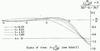
Fig. 8. Progress in lime of dimensionless moment in the frontal part of an infinitely wide floating glacier
The scale of time T of the deformation progression varies from one glacier to another proportional to μ/h, i.e.

Substituting μ from Equation (12), where τ and θ are now regarded as representative mean values for the glacier, and substituting

(where the constant of proportionality is 1 bar3 year), which shows that the thinner and colder a floating glacier is, the greater is the time scale T, i.e. the longer the periods that pass until a certain state of the deformation progression is attained.
In order to get an idea of the periods required for producing considerable deflections, let us calculate some representative values of the factor

Putting d i = 0.9, the values for f shown in Table II arc obtained. If d i = 0.8, the values in the table should he divided by about 3.
Table II. Timefactor f in Years as Function of Thickness h and Temperature θ

By means of the values in Table II and the curves in Figure 6 it can be seen that a 600-m thick glacier having a mean temperature of −4°C and a relative density of 0·9 (this glacier represents the ice streams of West Greenland) will attain a deflection of 30 m (a twentieth of the thickness) after about 0·29 year = 3·5 months, while a 200-m thick glacier having a mean temperature of −12°C—and a relative density of 0·8—(representing an Antarctic ice shelf)—will attain a relative deflection of the same magnitude only after about 19 years. These values are, of course only to be taken as orders of magnitude.
From Equations (26), (27) and (to) we get the following expression for the stress differenceσ′11−σ′22
From this equation and Figures 6 and 8 the progress in time of σ′11−σ′22 may be obtained. Putting d i = 0.9 and putting

Fig. 9. Progress in time of the dimensionless stress-difference σ′11−σ′22in the frontal part of an infinitely wide floating glacier
As seen from Equation (28), the maximum value of the shear stress σ′12 occurs at the middle surface of the glacier (x′2 = 0) and has the magnitude 1.5Q′. The progress in time of the maximum shear stress may consequently be obtained by multiplying the values given by the curves in Figure 7 by the factor 1·5. Figure 7 shows that the shear stress is maximum at a cross-section situated at a distance of about half the thickness of the glacier from the front, and that the shear stress at this cross-section increases in time. From the above considerations, in conjunction with Equation (29) it will be seen that the effective shear stress attains the greatest values at a cross-section situated at a distance from the front of about the thickness of the glacier.
6. Fracture Criterion
As introduction to a discussion of where and when the state of stress in the glacier becomes critical, from the point of view of fracture, some general remarks on the fracture criterion for ice would be appropriate. A reasonable criterion for the fracture of ice is that the ultimate strength is attained when the effective shear stress τ has reached a certain critical value, which is a function of the mean normal stress
At present a formula expressing the fracture criterion cannot be set up, but the criterion can be given the following general formulation: the higher the temperature, the greater the effective shear stress and the greater the mean normal stress (tensile positive), the shorter will be the time until fracture occurs.
As stated above, the effective shear stress is greatest at a cross-section situated at a distance from the front of about the thickness of the glacier. At the upper surface the mean normal stress is greatest, and consequently the ice will fracture at the surface, at which a crack starts opening. Consequently, the stresses in the untracked part of the cross-section increase, resulting in increased deformation rates. After some time, this procedure will lead to total fracture, resulting in the formation of an iceberg. The width of the iceberg produced is of the same order of magnitude as the thickness of the glacier. The magnitude of the maximum effective shear stress may be obtained from Equation (29) and Figure (9). It is approximately
where k depends on d i. The Table III shows values of τ for different values of d i and h. The two rows correspond to d i = 0.9 (an approximate value for the ice streams of West Greenland) and d i = 0.8 (an approximate value for the ice shelves of Antarctica). The thickness of the ice streams of West Greenland is of the order of magnitude of 200–700 m, that of the fronts of the Antarctic ice shelves of the order of magnitude of 200–300 m. From Table III the maximum effective shear stress is found to be 1–3 bars in both cases.
Table III. Maximum Effective Shear Stress (In Bars) as a Function of Relative Density d iand thickness h

According to Reference PounderPounder (1965, p. 96) the tensile strength of ice, as obtained from short-time tests, is 15 bars. The test results may be larger or smaller than this value by a factor of two or three. Due to inhomogeneities, which must exist inside a large ice body as a glacier, the tensile strength of the glacier ice must be less than, say, 10 bars, to which corresponds an effective shear stress of 10/√3≈6 bars. On these grounds it seems reasonable to postulate, that an effective shear stress of the order of magnitude of 1–3 bars acting for a long time under tensile conditions will lead to fracture.
The question as to when the fracture occurs cannot be answered until more is known about the long-time strength of ice, but according to the above discussion of the fracture criterion, it may be stated that the thinner and colder a floating glacier is the longer are the intervals between one calving and another.
6. Observations Supporting the Proposed Theory of Calving
Evidence of a large downward deformation of the frontal part of a glacier at the stages preceding calving, is provided by a couple of aerial photographs of Rink Gletscher in northwestern Greenland, taken in June 1964 (Figs. 10 and 11). As will be seen from the photographs, the glacier has calved during the period of 13 days that has elapsed between the first and the second photographs.

Fig. 10. Rink Gletscher, 9 June 1964. (Geodetisk Institut. Denmark, copright)

Fig. 11. Rink Glctscher, 22 June 1964. (Geodætisk Institut, Denmark. copyright)
The topographical maps shown in Figures 12 and 13 are based on the aerial photographs. The mapping was carried out by means of a stereothope. In the absence of the necessary fixed points, only vertical adjustments of the stereoscopic models have been carried out so that four points at sea-level have been used as fixed points with known levels. The scale of the maps was determined on the basis of the flight altitude. For these reasons the maps are, of course, somewhat inaccurate. Looking at the maps, one observes that south of the dotted line shown in Figure 12, the level of the glacier’s surface is practically constant (about 80 m above sea-level). This is quite likely because this part of the glacier is floating. Considering the map and the longitudinal section shown in Figures 12 and 14 respectively, it can be seen that at the front of the glacier the upper surface is almost at the water level. Consequently, the downward deflection of the front amounts to about 80 m. On the other hand, the part of the glacier immediately behind the front has moved about 20 m upwards. This is precisely the sort of deformation predicted by the theory. Another thing supporting the theory, as will be seen from Figure 10, is the presence of recently opened crevasses near, and parallel to, the front, indicating tensile stresses at this place. Such crevasses are apparent from aerial photographs of all glaciers terminating in water.

Fig. 12. Topographical map of Rink Gletscher based on the photography carried out 9 gone 1964

Fig. 13. Topographical map of Rink Gletscher based on the photography carried out 22 June 1964

Fig. 14. Longitudinal section of Rink Gletscher at the position shown in Figure 12
Having mentioned the things supporting the theory, it must in fairness be admitted that not all the surface features observable on the photographs can be explained. The existence of the smaller waves behind the large one at the front is not predicted by the theory, which gives a wave-length of the undulations of several times the thickness of the glacier. The wavelength of the undulations in Figure 12 is of the same order of magnitude as the thickness of the glacier.
Another result of the theory, which is supported by observations from nature is that the thinner and colder a floating glacier is, the longer are the intervals between one calving and another. This agrees with the observation that calving from the relatively cold and thin floating ice fronts in north Greenland (e.g. Melville Bugt) and Antarctica, occurs at longer intervals than calving from the warmer and, especially, thicker glaciers terminating in Disko Bugt and the Umanak distrikt in western Greenland.
7. Discussion of other Calving Mechanisms
Several theories of the causes of calving have been given in the past. Some of these will be discussed briefly below.
-
a. Buoyancy effects. These arise either from the oblique, downward movement of the front into the sea or from tide variations. Common to these effects are that the greatest stresses produced by them occur at the point of transition from the grounded part of the glacier to the part afloat, which means that the width of the icebergs should be equal to the length of the floating part of the glacier. This is evidently not the case as regards the icebergs originating from the Antarctic ice shelves.
-
b. Effect of storm waves. The action of waves at the ice front itself can hardly result in stresses which can lead to calving. However, the waves will also produce pressure fluctuations along the lower surface of the glacier. Now, the pressure fluctuations decrease very rapidly with the distance below the sea surface, and at a depth equal to the wave-length they have practically disappeared. Wave-lengths of 200–300 m are the maximum reported for ocean waves. Below a depth of this magnitude, significant pressure fluctuations will not occur. Since the thickness of most of the fronts of floating glaciers and ice shelves is more than 200 m we can conclude that the action of storm waves can hardly explain the breaking of big icebergs from the ice front.
8. Conclusion
The theory of calving advanced in this paper seems to agree with observations from the ice streams of western Greenland, especially with observations from such ice streams as the Jakobshavn Isbrm and Rink Gletscher, which, most likely, have floating fronts. On the other hand, the theory does not explain directly the periodical break-up of large portions of the Antarctic ice shelves. A possible explanation of this feature is that, when the first iceberg has loosened from the front, the adjoining part of the shelf is not in equilibrium and, consequently, breaks off, and so on.
It should be pointed out that, of course, not all of the ice calved from the floating glaciers of the world is formed in the way proposed in this paper. Many small icebergs are, for example, produced by pieces falling down from the upper part of the ice front.
Finally, it should be mentioned that a consequence of the theory proposed is that the size of the icebergs as well as the frequency of calving depends solely on the thickness, the temperature, and the density of the glacier. Consequently, the loss of ice by calving depends on these three quantities only. The width of the glacier will of course influence the calving process to some degree. But if the width is just a few times the thickness of the glacier, the influence is believed to be small.
9. Acknowledgement
I wish to thank Københavns Universitets Geografiske Institut, in particular Dr Tyge Møller, for placing at my disposal maps, aerial photographs and the Zeiss Stereothop of the Institut, for the mapping work.


