


1. Introduction
In a circular pipe, the laminar entrance flow, which precedes the fully developed Poiseuille flow, encapsulates the general features of viscous flow, which makes it one of the standard problems in fluid dynamics. Despite its limited applicability in practical scenarios, numerous studies have focused on deriving an analytical solution connecting to the exact solution of Poiseuille flow. Typically, the momentum equation governing the entrance flow is reduced to the parabolised Navier–Stokes equation. Similar to the boundary layer theory, this equation neglects the axial gradient of linear dilatation and radial variation of pressure in the full Navier–Stokes equations.
Numerous studies have described and summarised analytical solutions to the parabolised Navier–Stokes equation for entrance flow (Fargie & Martin Reference Fargie and Martin1971; Mohanty & Asthana Reference Mohanty and Asthana1978; Reci, Sederman & Gladden Reference Reci, Sederman and Gladden2018). These solutions can be divided into two categories: category (i) involves linearising the inertia term with axial velocity in the momentum equation, yielding solutions as series functions (Langhaar Reference Langhaar1942; Sparrow, Lin & Lundgren Reference Sparrow, Lin and Lundgren1964; Wiginton & Wendt Reference Wiginton and Wendt1969; Boussinesq Reference Boussinesq1981). Category (ii) assumes the growth of the boundary layer along the pipe wall. Here, the inviscid core flow outside this boundary layer accelerates to satisfy the continuity equation. As the boundary layer merges at the central axis, the velocity profile adapts to the fully developed flow (Schiller Reference Schiller1922; Campbell & Slattery Reference Campbell and Slattery1963; Schlichting Reference Schlichting1969; Fargie & Martin Reference Fargie and Martin1971; Gupta Reference Gupta1977; Mohanty & Asthana Reference Mohanty and Asthana1978). Regardless of the theoretical method employed, these analytical solutions are consistent with experimental measurements of the pressure drop and central axis velocity (Reshotko Reference Reshotko1958; Emery & Chen Reference Emery and Chen1968; Fargie & Martin Reference Fargie and Martin1971; Mohanty & Asthana Reference Mohanty and Asthana1978; Al-Nassri & Unny Reference Al-Nassri and Unny1981). In each case, the maximum axial velocity within the pipe cross-section is consistently located on the central axis and accelerates to the fully developed value. Furthermore, the velocity distributions measured using laser Doppler velocimetry (Berman & Santos Reference Berman and Santos1969) and particle tracers (Atkinson, Kemblowski & Smith Reference Atkinson, Kemblowski and Smith1967) have also demonstrated the existence of the peak velocity on the central axis.
However, numerical results from the full Navier–Stokes equations often reveal that the maximum velocity is located near the wall, off the central axis, for a short distance downstream from the inlet (Friedmann, Gillis & Liron Reference Friedmann, Gillis and Liron1968; Atkinson et al. Reference Atkinson, Brocklebank, Card and Smith1969; Wagner Reference Wagner1975; Pagliarini Reference Pagliarini1989; Dombrowski et al. Reference Dombrowski, Foumeny, Ookawara and Riza1993; Lorenzini & Saro Reference Lorenzini and Saro1999; Durst et al. Reference Durst, Ray, Ünsal and Bayoumi2005; dos Santos & Figueiredo Reference dos Santos and Figueiredo2007). This phenomenon is termed velocity overshoot. Velocity overshoot is observed in the laminar entrance flow across a wide range of Reynolds numbers ( $0< Re \le 2000$), as predicted by numerical methods. Recently, Reci et al. (Reference Reci, Sederman and Gladden2018) measured the radial distribution of axial velocities close to the inlet using magnetic resonance (MR) velocimetry for
  $120 \le Re \le 1100$. Their experiments confirmed the existence of velocity overshoot in all the considered cases, with the location and magnitude of the velocity overshoot aligning with numerical predictions derived from the full Navier–Stokes equations.
In high  $Re$ entrance flows, the full Navier–Stokes equations are often parabolised based on Prandtl's boundary layer theory, an approach regarded as valid. Therefore, the velocity overshoot observed in numerical solutions of the full Navier–Stokes equations for high
  $Re$ flows should also be discernible in analytical solutions derived from the parabolised Navier–Stokes equation. The absence of velocity overshoot in analytical solutions need not be due to the omitted terms in the full Navier–Stokes equations. The velocity overshoot was experimentally confirmed for
  $Re = 1100$, a considerably high value, suggesting that it should also be evident in solutions of the parabolised Navier–Stokes equation.
The velocity profiles resulting from inertia term linearisation in the analytical solutions of category (i) are monotonically decreasing functions from the central axis along the radius; thus, the maximum velocity is located on the central axis. In the analytical solutions of category (ii), the maximum velocity consistently occurs in the inviscid core outside the boundary layer. After the boundary layer merges at the central axis, a monotonic convex velocity profile is maintained until the flow is fully developed; hence, a velocity overshoot is impossible. As a result, there is a necessity for a new method to establish an analytical solution that can account for the velocity overshoot.
This study presents a new approach for analysing the parabolised Navier–Stokes equation, marking the first instance of identifying the existence of velocity overshoot through an analytical solution. The momentum equation was analytically integrated by dividing the pipe cross-section into two distinct flow regions: near the wall and the remainder. Approximations were introduced considering the physical characteristics of each region. Figure 1 illustrates the velocity development in the two flow regions. In the central region, the study assumed that inertia is counterbalanced not only by the pressure gradient but also by the shear force term, commonly neglected in the inviscid core introduced in category (ii). In addition, the axial velocity was replaced with the central axis velocity within this region. This substitution results in a linearised momentum equation facilitating analytical integration along the radial direction. In this context, the central flow is not inviscid; the inertia term diminishes and eventually vanishes as the flow develops. Therefore, this study refers to the central flow region as the inertia-decaying core. The boundary layer thickness from the wall cannot be assigned due to the radial gradient of the axial velocity within the inertia-decaying core. Shear stress dominates the flow immediately adjacent to the wall. Thus, in contrast to category (ii), the momentum equation for this region was linearised by ignoring the inertia term. Here, the pressure gradient is counterbalanced only with the shear stress derivative, and the flow region is termed the wall shear layer. A mathematically continuous axial velocity solution across the entire pipe cross-section can be obtained by employing a matching condition, thus ensuring equality of velocity and its gradient at the interface between the inertia-decaying core and wall shear layer. The flow within the wall shear layer corresponds to the Couette flow with a forward pressure gradient, where the interface velocity is a boundary traction velocity. In the Couette flow, the velocity overshoot is possible according to the interplay between interface velocity and pressure gradient. An extremely high pressure gradient near the inlet downstream facilitates the emergence of a velocity overshoot. As the flow progresses, the interface velocity accelerates while the pressure gradient decreases. As a result, the velocity overshoot disappears, and the maximum velocity eventually shifts to the central axis. The streamfunction, expressed analytically using the axial velocity as a continuous function across both regions, enables the derivation of radial velocity upon differentiation. The accuracy of this analytical solution was verified through comparison with published experimental data concerning the central axis velocity and pressure drop. Specifically, the velocity overshoot was compared with the recent MR velocimetry measurements to confirm the validity of the analytical solution. Moreover, alterations in the velocity profile throughout flow development were investigated in detail.

Figure 1. Schematic of the velocity development in a circular pipe laminar entrance flow, as predicted by the present analytical solution. The maximum velocity within the pipe cross-section initially appears near the wall and subsequently shifts towards the central axis as a uniform velocity is re-established in the central region. During this transition, the velocity profile in the central region changes from a concave to a convex shape, eventually settling into a monotonic convex profile that aligns with the fully developed parabolic function.
The parabolised Navier–Stokes equation exhibits self-similarity with respect to  $Re$, implying that
  $Re$ is not an independent flow parameter and is incorporated into the dimensionless variables. Although only limited data were available, self-similarity was investigated using the MR velocimetry measurement data, thereby examining the inherent limitations of the analytical solution derived from parabolising the momentum equations. As
  $Re$ decreases, the influence of the terms neglected from the full Navier–Stokes equations increases, and according to the MR velocimetry measurements, this effect becomes more pronounced closer to the inlet. Because the present study relying on the parabolised Navier–Stokes equation is unsuitable for low
  $Re$ flows, further studies are necessary to specify the
  $Re$ range that ensures the accuracy of the analytical solution. This can be accomplished through numerical and/or experimental methods.
2. Derivation of the analytical solution
2.1. Governing equations
To non-dimensionalise the governing equations, dimensionless variables are introduced as follows:
 \begin{equation} {\xi} = \frac{x}{D Re},\quad \eta = \frac{r}{D/2},\quad U= \frac{u}{u_b}, \quad V= \frac{v}{u_b /Re}, \quad P= \frac{p}{\rho u^2_b /2}, \end{equation}
where  $\rho$,
  $D$ and
  ${u_b}$ represent the fluid density, the pipe diameter and the mean velocity, respectively. The Reynolds number, expressed as
  $Re= ( \rho D {u_b} )/\mu$, is defined using these reference values with the fluid viscosity
  $\mu$. All values follow conventional forms (Fargie & Martin Reference Fargie and Martin1971), and the reference pressure is assigned to the dynamic pressure consistent with the friction factor definition. The dimensionless continuity equation and full Navier–Stokes equations are transformed as follows:
 $$\begin{gather} \frac{\partial U}{\partial \xi} + \frac{2}{\eta} \frac{\partial (\eta V)}{\partial \eta} =0, \end{gather}$$
 $$\begin{gather}U \frac{\partial U}{\partial \xi} + 2V \frac{\partial U}{\partial \eta} =- \frac{1}{2} \frac{\partial P}{\partial \xi} + \frac{1}{Re^2} \frac{ {\partial}^2 U}{\partial {\xi}^2} + \frac{4}{\eta} \frac{\partial }{\partial \eta} \left(\eta\frac{\partial U}{\partial \eta} \right)\!, \end{gather}$$
 $$\begin{gather}\frac{1}{Re^2} \left( U \frac{\partial V}{\partial \xi} + 2V \frac{\partial V}{\partial \eta} \right)=- \frac{\partial P}{\partial \eta} + \frac{1}{Re^2} \left[ \frac{1}{Re^2} \frac{ {\partial}^2 V}{\partial {\xi}^2} + \frac{4}{\eta} \frac{\partial}{\partial \eta} \left( \eta \frac{\partial V}{\partial \eta} \right) - \frac{4V}{{\eta}^2} \right]\!. \end{gather}$$
The Reynolds number solely governs the flow. For  $Re \gg$ 1, the axial gradient of linear dilatation in (2.3) can be ignored, while (2.4) shows the radial pressure variation to be negligible. Consequently, similar to the boundary layer equation, the axial momentum equation (2.3) simplifies to the parabolised Navier–Stokes equation as follows:
 \begin{equation} U \frac{\partial U}{\partial \xi} + 2V \frac{\partial U}{\partial \eta} =- \frac{1}{2} \frac{{\rm d} P}{{\rm d} \xi} + \frac{4}{\eta} \frac{\partial }{\partial \eta} \left( \eta \frac{\partial U}{\partial \eta} \right)\!. \end{equation}
The Reynolds number disappears and is grouped within the dimensionless axial coordinate and radial velocity, as shown in (2.1a–e), indicating the dimensionless coordinate system's self-similarity with respect to  $Re$. In the entrance flow region, flows with different
  $Re$ values will exhibit similar velocity profile shapes at specific
  $\xi$ positions. However, as
  $Re$ decreases, the omitted terms in the full Navier–Stokes equations gain significance, undermining the self-similarity.
To integrate the axial momentum equation analytically, the flow field is divided into two regions, similar to the previous studies in category (ii); however, distinct assumptions are introduced for each region. Within the inertia-decaying core, the radial variation of axial velocity is markedly diminished, which is attributed to the restricted wall effect, rendering it insignificant in comparison with the axial variation; furthermore, the radial velocity is negligible. Thus,  $U_c (\partial U_c / \partial \xi ) \gg 2 V_c ( \partial U_c / \partial \eta )$, where subscript
  ${\it c}$ indicates the inertia-decaying core. Ignoring radial variation, the inertia term can be approximated by the central axis velocity
  $U_0$, which is the usual assumption in the inviscid core (Fargie & Martin Reference Fargie and Martin1971; Gupta Reference Gupta1977; Mohanty & Asthana Reference Mohanty and Asthana1978; Smith & Cui Reference Smith and Cui2004), leading to
 \begin{equation} U_c \frac{\partial U_c}{\partial \xi} + 2 V_c \frac{\partial U_c}{\partial \eta} \approx \frac{1}{2} \frac{{\rm d} U_0^2}{{\rm d} \xi}. \end{equation}
Substituting (2.6) into the momentum equation (2.5), we obtain
 \begin{equation} \frac{1}{2} \frac{{\rm d} U_0^2}{{\rm d} \xi} =- \frac{1}{2} \frac{{\rm d} P}{{\rm d} \xi} + \frac{4}{\eta} \frac{\partial }{\partial \eta} \left( \eta \frac{\partial U}{\partial \eta} \right)\!. \end{equation}
In contrast to the case of the inviscid core, the shear stress derivative remains, prevailing even at the symmetric central axis where the shear stress is zero. This is confirmed in the fully developed flow, where the shear stress derivative is constant across the entire pipe section. The velocity profile changes from concave to convex depending on the relative magnitudes of the pressure gradient and the inertia term.
The shear stress prevails in the force balance near the pipe wall owing to the no-slip condition, and the inertia terms are disregarded different from the previous studies in category (ii). A sudden change of the uniform velocity profile at the pipe inlet edge may cause a significant momentum difference. This effect is assumed to be confined locally at the inlet edge, and it may cause inaccuracies of present analytical solution in this region. The momentum equation for the wall shear layer is simplified to
 \begin{equation} 0 =- \frac{1}{2} \frac{{\rm d} P}{{\rm d} \xi} + \frac{4}{\eta} \frac{\partial }{\partial \eta} \left( \eta \frac{\partial U_w}{\partial \eta} \right)\!, \end{equation}
where subscript  ${\it w}$ indicates the wall shear layer. An inertia-decaying core, where the flow progresses with increasing velocity and decreasing pressure gradient, is situated adjacent to the wall shear layer. Velocities at the interface of the two flow regions overlap, and the same pressure gradient governs both flows. Under these conditions, the flow in the wall shear layer can be regarded as a Couette flow with varying boundary velocity and pressure gradient. The forward pressure gradient results in a convex velocity profile, and a velocity overshoot arises from the prevailing effect of the pressure gradient over the interface velocity.
2.2. Velocity solutions
The interface radius between the two flow regions, denoted as  ${\eta }_{\delta } ( \xi )$, is a new unknown variable, which separates the flow velocity as follows:
 \begin{equation} U (\xi , \eta ) = \left\{\begin{array}{@{}ll@{}} U_c ( \xi , \eta ), & 0 \le \eta \le {\eta}_{\delta} \\ U_w ( \xi , \eta ), & {\eta}_{\delta} \le \eta \le 1 \end{array}\right.\!. \end{equation}
As the wall shear layer extends to the central axis, the inertia-decaying core shrinks. When the inertia term in the inertia-decaying core sufficiently diminishes, the momentum equations for each flow region are approximately equivalent, and the velocity profiles overlap significantly. Beyond this point, the interface radius no longer changes, and the flow becomes fully developed as the inertia term vanishes completely.
The momentum equation (2.5) is approximated for each flow region, and the resultant equations (2.7) and (2.8) can be integrated analytically. Two boundary conditions are available – one for the inertia-decaying core at the symmetric central axis and the other for the wall shear layer at the no-slip wall – expressed as follows:
 \begin{equation} \frac{\partial U_c ( \xi ,0)}{\partial \eta} =0, \quad U_w ( \xi ,1) =0. \end{equation}
At the interface radius, the velocities and their slopes (shear stresses) must be equal, ensuring a continuous function of velocity across the two regions
 \begin{equation} U_c ( \xi , {\eta}_{\delta}) = U_w ( \xi , {\eta}_{\delta}), \quad \frac{\partial U_c ( \xi , {\eta}_{\delta})}{\partial \eta} = \frac{\partial U_w ( \xi , {\eta}_{\delta})}{\partial \eta}. \end{equation}
Applying the boundary conditions (2.10a,b) and interface-matching conditions (2.10a,b), four integral coefficients are determined, and the velocities are yielded as
 $$\begin{gather} U_c ( \xi ,\eta )=- \frac{D_{\! P}}{32} (1- {\eta}^2) + \frac{D_U}{32} {\eta}^2 - \frac{D_U}{32} {\eta}_{\delta}^2 (1- \ln {\eta}_{\delta}^2), \end{gather}$$
 $$\begin{gather}U_w ( \xi ,\eta )=- \frac{D_{\! P}}{32} (1- {\eta}^2) + \frac{D_U}{32} {\eta}_{\delta}^2 \ln {\eta}^2, \end{gather}$$
where  $D_{\! P} ( \xi )$ and
  $D_U ( \xi )$ are introduced to reduce the complexity of the expression and are defined as follows:
 \begin{equation} D_{\! P} ( \xi ) \equiv \frac{{\rm d} P}{{\rm d} \xi},\quad D_U ( \xi ) \equiv \frac{{\rm d} U_0^2}{{\rm d} \xi}. \end{equation}
The central axis velocity can be deduced from (2.12) at  $\eta = 0$, from which the pressure gradient
  $D_P ( \xi )$ is expressed as
 \begin{equation} D_{\! P} ( \xi ) =-32 U_0 - D_U {\eta}_{\delta}^2 (1- \ln {\eta}_{\delta}^2). \end{equation}
The pressure gradient is removed from (2.12) and (2.13) to obtain
 $$\begin{gather} U_c ( \xi ,\eta )= U_0 ( 1- {\eta}^2 ) + \frac{D_U}{32} [ 1- {\eta}_{\delta}^2 ( 1- \ln {\eta}_{\delta}^2 )] {\eta}^2, \end{gather}$$
 $$\begin{gather}U_w ( \xi ,\eta )= U_c ( \xi ,\eta ) + \frac{D_U}{32} [{\eta}_{\delta}^2 (1- \ln {\eta}_{\delta}^2)- {\eta}^2 + {\eta}_{\delta}^2 \ln {\eta}^2]. \end{gather}$$
The velocity at an axial position  $\xi$ is represented by a function of
  $\eta$, with two axially varying parameters
  $U_0 ( \xi )$ and
  ${\eta }_{\delta } ( \xi )$. The remaining
  $D_U ( \xi )$ is calculated from
  $U_0 ( \xi )$. Two additional equations are needed to determine these unknown parameters.
The continuity and the momentum equations integrated over the pipe cross-section are referred to as global equations. They are useful in analysing the internal flow, and the equations necessary to solve  $U_0 ( \xi )$ and
  ${\eta }_{\delta } ( \xi )$ are derived from them. The continuity equation (2.2) is integrated over the pipe cross-section
 \begin{equation} \frac{{\rm d}}{{\rm d} \xi} \int_0^1 U( \xi,\eta ) \eta \,{\rm d} \eta + 2 \int_0^1 \frac{\partial ( \eta V)}{\partial \eta} \, {\rm d} \eta =0. \end{equation}
Due to the boundary conditions, the second term of the left-hand side of (2.18) becomes zero. Integrating equation (2.18) over  $\xi$ results in
 \begin{equation} \int_0^1 U( \xi ,\eta ) \eta \,{\rm d} \eta = {\rm constant}. \end{equation}
Because the left-hand side of (2.19) represents the total mass flow rate at any  $\xi$, by applying the uniform inlet velocity condition, the constant on the right-hand side is 1/2. Eventually, the global continuity equation can be derived by substituting the velocity equations (2.16) and (2.17) and integrating analytically for each region
 \begin{equation} \int_0^{{\eta}_{\delta}} U_c( \xi ,\eta ) \eta \, {\rm d} \eta + \int_{{\eta}_{\delta}}^1 U_w( \xi ,\eta ) \eta \, {\rm d} \eta = \tfrac{1}{2}. \end{equation}
Following mathematical modification, the global continuity equation can be expressed as
 \begin{equation} \frac{{\rm d} U_0^2 ( \xi )}{{\rm d} \xi} = \frac{32 ( U_0 -2) }{{\eta}_{\delta}^2 ( 1- {\eta}_{\delta}^2 + \ln {\eta}_{\delta}^2)}. \end{equation}
In addition, the momentum equation (2.5) is integrated over the pipe cross-section
 \begin{equation} \frac{{\rm d}} {{\rm d} \xi} \int_0^1 U^2 \eta \, {\rm d} \eta +2 \int_0^1 \frac{\partial ( \eta UV)}{\partial \eta} {\rm d} \eta =- \frac{D_{\! P}}{2} \int_0^1 \eta \, {\rm d} \eta + 4 \int_0^1 \frac{\partial}{\partial \eta} \left( \eta \frac{\partial U}{\partial \eta} \right) {\rm d} \eta. \end{equation}
Here, the left-hand side of (2.5) is switched to conservative form using the continuity equation. The second term of the left-hand side is removed owing to the boundary conditions, and the global momentum equation is obtained
 \begin{equation} \frac{{\rm d} \varTheta ( \xi )}{{\rm d} \xi} =-\frac{D_{\! P}}{4} + 4 \left( \eta \frac{\partial U_w}{\partial \eta} \right)_{\eta = 1}, \end{equation}
where the global momentum  $\varTheta ( \xi )$ is defined as
 \begin{equation} \varTheta ( \xi ) = \int_0^1 U^2 \eta \, {\rm d} \eta. \end{equation}
Substituting (2.15), (2.17) and (2.21) into (2.23), the global momentum equation becomes
 \begin{equation} \frac{{\rm d} \varTheta (\xi )}{{\rm d} \xi} = \frac{8 ( U_0 -2)}{1- {\eta}_{\delta}^2 + \ln {\eta}_{\delta}^2}. \end{equation}
The global momentum in (2.24) is partially integrated by applying (2.16) and (2.17), resulting in
 \begin{align} \varTheta (\xi ) = \frac{2}{3} - \frac{( U_0 -2) ( 1- {\eta}_{\delta}^2)^2 }{6 ( 1- {\eta}_{\delta}^2 + \ln {\eta}_{\delta}^2)}+ \frac{( U_0 -2)^2 ( 2+3 {\eta}_{\delta}^2 -6 {\eta}_{\delta}^4 + {\eta}_{\delta}^6 +6 {\eta}_{\delta}^2 \ln {\eta}_{\delta}^2) }{12 ( 1- {\eta}_{\delta}^2 + \ln {\eta}_{\delta}^2)^2}. \end{align}
 There are three unknowns ( $U_0 ( \xi )$,
  ${\eta }_{\delta } ( \xi )$ and
  ${\it \varTheta } ( \xi )$) to solve, and we have two first-order ordinary differential equations (2.21) and (2.25) and one algebraic equation (2.26). To create a closed form for the equation set, three inlet conditions are required to integrate the differential equations. The central axis velocity at the inlet is
  $U_0 (0)= 1$ due to the uniform inlet velocity condition, and applying it to (2.24) results in
  $\varTheta ( 0 )= 1/2$. Because the wall shear layer takes place from the pipe wall, the interface radius at the inlet is
  ${\eta }_{\delta } ( 0 )= 1$. The ordinary differential equations (2.21) and (2.25) were integrated using the fourth-order Runge–Kutta method. At each prediction and correction step of the Runge–Kutta integration,
  ${\eta }_{\delta } ( \xi )$ was calculated from (2.26) using the bisection method.
2.3. Supplementary equations
The total pressure drop from the inlet can be calculated by integrating equation (2.23) with respect to  $\xi$, which is expressed as follows:
 \begin{equation} {\rm \Delta} P ( \xi ) = 4 \left[ {\it \varTheta} ( \xi ) - \tfrac{1}{2} \right] + \int_0^{\xi} (32 U_0 - D_U {\eta}_{\delta}^2 \ln {\eta}_{\delta}^2)\,{\rm d} \hat{\xi}. \end{equation}
The term within the square brackets represents the net change in the inertia force, and the integral is the shear force at the pipe wall. The fourth-order Runge–Kutta method was adopted for the integration.
The velocity functions are continuous across two flow regions, and the streamlines can be obtained using the streamfunction defined as
 \begin{equation} \varPsi ( \xi, \eta ) = \tfrac{1}{2} \int_0^{\eta} U( \xi , \eta ) \hat{\eta} \, {\rm d} \hat{\eta}. \end{equation}
Substituting (2.16) and (2.17) into (2.28) yields the following streamfunctions:
 $$\begin{gather} \varPsi_c ( \xi, \eta ) = \frac{U_0}{8} ( 2- \eta^2) \eta^2 + \frac{D_U}{256} [(1- {\eta}_{\delta}^2)^2 + {\eta}_{\delta}^2 ( 1- {\eta}_{\delta}^2 + \ln {\eta}_{\delta}^2)] {\eta}^4, \end{gather}$$
 $$\begin{gather}\varPsi_w ( \xi , \eta ) = {\it \varPsi_c} ( \xi , \eta ) + \frac{D_U}{256} [ {\eta}_{\delta}^4 +2 {\eta}_{\delta}^2 (1- \ln {\eta}_{\delta}^2) {\eta}^2 - {\eta}^4 - 2 {\eta}_{\delta}^2 (1 - \ln {\eta}^2) {\eta}^2]. \end{gather}$$
The radial velocity can be determined by differentiating the streamfunction
 \begin{equation} V ( \xi, \eta ) =- \frac{1}{\eta} \frac{\partial \varPsi ( \xi , \eta ) }{\partial \xi}. \end{equation}
The central differencing method was used for this differentiation.
3. Results and discussion
Initially, the validity of the analytical solution was confirmed by comparing its limiting values with the theoretical values associated with a fully developed flow. Subsequently, its accuracy was verified through a comparison with previously published experimental results. The prediction of the velocity overshoot was examined using the measurements recently published by Reci et al. (Reference Reci, Sederman and Gladden2018). Finally, the transition of the velocity profile, including the velocity overshoot during flow development, was investigated in detail using the analytical solution.
3.1. Accuracy of the analytical solutions
The current approach was established without incorporating information on the fully developed flow. Consequently, the analytical solution's validity is confirmed by comparing the data at the conclusion of the entrance flow with the theoretical values of the fully developed flow. Figure 2 depicts the axial variations of representative dependent variables, and table 1 lists the analytical solution values converging to predefined fully developed conditions for comparison with theoretical values.

Figure 2. Axial variation of representative dependent variables converging to the fully developed condition. The entrance length is estimated as  ${\xi }_e = 0.0586$, which is within the range of previously reported values. The validity of the analytical solution can be confirmed, as all limiting values converge to the theoretical values, even without prior information concerning the fully developed condition.
Table 1. Limiting values of representative dependent variables in the analytical solution converging to the fully developed flow. Data extracted at the positions corresponding to the 99 % ratio (ratio of the central axis velocity to the fully developed value,  $U_0/U_{0,F}$), which is the conventional definition of the entrance length, and the 99.99 % ratio is compared with the theoretical values of the fully developed flow. Minor discrepancies exist between the values at the end of the entrance length and those corresponding to the theoretical fully developed condition; however, at the 99.99 % ratio, the differences are negligible.

Typically, the end of the entrance length is defined as the position where the central axis velocity attains 99 % of the fully developed velocity. By this criterion, the entrance length is  ${\xi }_e = 0.0587$, which falls within the range summarised by Durst et al. (Reference Durst, Ray, Ünsal and Bayoumi2005) after reviewing numerous studies. Their work, encompassing experimental, analytical and numerical approaches, aimed to provide quantitative information on the relationship between entrance length and Reynolds number. Their numerical investigation based on the full Navier–Stokes equations yielded the following analytical relationship:
 \begin{equation} \frac{{\xi}_e}{Re} = [ {0.619}^{1.6} + (0.0567 Re)^{1.6}]^{1/1.6}. \end{equation}
Except at very low  $Re$, the first term inside the bracket is negligible. For instance, at
  $Re = 100$, it contributes less than 2 %. Hence, the relation can be simplified to
  ${\xi }_e \approx$ 0.0567, which only deviates by 3.4 % from the present analytical solution.
As shown in figure 2, the variables  $U_0 ( \xi )$,
  $\varTheta ( \xi )$ and
  $D_{\! P} ( \xi )$ converged to their limiting values, and no more changes were observed. The inertia term
  $D_U ( \xi )$, scaled by log in the figure, decreases sufficiently from infinity to less than 1, and it heads to zero. Marginal differences from the fully developed flow exist in the values at the 99 % velocity condition; however, at the 99.99 % condition, the values are consistent with the fully developed ones (table 1). The pressure drop from the inlet increases linearly except at the section close to the inlet. These results confirm the validity of the analytical solution.
The variation in the central axis velocity is compared with published experimental measurement results (Nikuradse Reference Nikuradse1950; Reshotko Reference Reshotko1958; Emery & Chen Reference Emery and Chen1968; Fargie & Martin Reference Fargie and Martin1971), and the analytical solution aligns well with the experimental results, as shown in figure 3. The maximum average error of the analytical solution relative to the experimental results for  $Re = 760$ (Fargie & Martin Reference Fargie and Martin1971) is 4 %, and the error reduces with the increasing
  $Re$. The pressure drops along the axial coordinate are shown in figure 4, and the analytical solution is consistent with the experiments. The average errors for each measurement marked in the figures were calculated as follows:
 \begin{equation} \varepsilon_{avg} = \frac{1}{n X_{ref}} \sum_{i=1}^n \sqrt{ ( X_{{exp},i} - X_{{cal},i})^2 }, \end{equation}
where  $X_i$ values are corresponding data points, and
  $X_{ref}$ denotes the reference value. For
  $U_{0, {ref}}$, the fully developed value
  $U_{0, {F}} = 2$ was applied, and
  ${\rm \Delta} P_{F} = 4.31$ (the pressure drop over total entrance length) is adopted for
  ${\rm \Delta} P_{ref}$.

Figure 3. Axial variation of the central axis velocity compared with the experimental data. The prediction by the analytical solution is consistent with the experimental measurements, and the average error is less than 4 %. The average errors were calculated using (3.2).

Figure 4. Axial variation in the pressure drop compared with the published experimental results. The analytical solution is consistent with the experiments, and the maximum average error is 8 %. The average errors were calculated using (3.2).
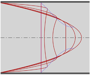
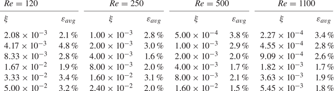
Most of the experimental studies have measured pressure drop and central axis velocity, and only a few have reported radial distribution of the axial velocity. Recently, Reci et al. (Reference Reci, Sederman and Gladden2018) experimentally corroborated the presence of velocity overshoot using MR velocimetry. Velocity profiles at a short distance from the inlet measured by MR velocimetry are presented in figure 5 and compared with the present analytical solutions. The Reynolds numbers in the experiment were  $Re =120$ (
 $\pm$10), 250 (
 $\pm$10), 500 (
 $\pm$20) and 1100 (
 $\pm$50), where the values within parentheses represent uncertainties; the velocity profiles were measured at six axial positions:
  $x/D = 0.25, 0.5, 1, 2, 4$ and 6. The six positions are transformed into the dimensionless coordinate
  $\xi$ using the four Reynolds numbers for comparison with the analytical solutions. The average errors for each velocity profile calculated by (3.2) are listed in table 2, where the reference velocity is
  $U_{ref} = U_{0, {F}}$, the fully developed value of the central axis velocity.

Figure 5. Velocity profiles at multiple axial positions compared with measurements using MR velocimetry. Experimental data were provided for four Reynolds numbers ( $Re = 120$, 250, 500, 1100), and for each
  $Re$ value, the velocity profiles were measured at six axial positions close to the inlet (
 $x/D = 0.25$, 0.5, 1, 2, 4, 6). To compare the measurements with the analytical solution, the six axial positions were transformed into the dimensionless coordinate
  $\xi$ using the corresponding
  $Re$, and the resultant
  $\xi$ sets are different for each
  $Re$; (a)
  $Re = 120$, (b)
  $Re = 250$, (c)
  $Re = 500$ and (d)
  $Re = 1100$.
Table 2. Average errors of the axial velocity profiles calculated by (3.2) and illustrated in figure 5. As  $Re$ increases, the error tends to decrease; that is, the greater the
  $Re$, the greater the accuracy of the analytical solution.
For the relatively low value of  $Re = 120$, velocities in the central zone at
  $\xi = 1.67\times 10^{-2}$ are well aligned with the measurements; however, the velocities are underestimated for smaller
  $\xi$ and overestimated for larger
  $\xi$, as quantified in table 2. At the position closest to the inlet,
  $\xi = 2.08\times 10^{-3}$, the discrepancies diminish. The velocity overshoot is discernible only for
  $\xi \le 4.17\times 10^{-3}$, close to the inlet. As shown in figure 5(b), the discrepancies of the analytical solution for
  $Re = 250$ are mitigated compared with
  $Re = 120$. The most consistent results are observed at
  $\xi = 4.0\times 10^{-3}$, revealing a trend similar to that in figure 5(a). For
  $Re = 500$ (c) and 1100 (d), the deviations are further reduced, representing the enhanced precision of the analytical solution at higher
  $Re$ values. Thus, the present analytical solution derived from the parabolised Navier–Stokes equation aligns more closely with the experiments at higher
  $Re$ and effectively identifies the velocity overshoot, a phenomenon not captured by previous analytical solutions.
The parabolised Navier–Stokes equation possesses inherent self-similarity with respect to the Reynolds number, and it can be examined using experimental data with the same  $\xi$ but different
  $Re$. Four
  $\xi$ positions (
 $\xi = 1.0\times 10^{-3}$,
  $2.0\times 10^{-3}$,
  $4.0\times 10^{-3}$ and
  $8.0\times 10^{-3}$) were available for
  $Re = 250$ and 500. Selected velocity profiles for these
  $Re$ values are illustrated in figure 6 and compared with the analytical solution. At a very short distance from the inlet, corresponding to
  $\xi = 1.0\times 10^{-3}$, a significant discrepancy emerges between the two velocity profiles for distinct
  $Re$ values, thus revealing the absence of self-similarity. As
  $\xi$ increases, the velocity data from MR velocimetry measurements for different
  $Re$ are closer to each other and the self-similarity becomes evident. Fundamentally, the parabolised Navier–Stokes equation cannot be applied to the flow close to the inlet where self-similarity is not satisfied, and the discrepancy between the analytical solution and the experiment is noticeable at
  $\xi = 1.0\times 10^{-3}$, as shown in figure 6. However, self-similarity is gradually re-established as
  $\xi$ increases, and the analytical solution increasingly aligns with the MR velocimetry measurements. For
  $Re = 1100$, the analytical solution is consistent with the experimental measurements, as shown in figure 5(d). This confirms that for high
  $Re$ flows, the analytical solution based on the parabolised Navier–Stokes equation with self-similarity is accurate, even close to the inlet. In figure 6, velocities measured just before the inlet are also depicted. Due to the non-ideality of the experimental apparatus, uniform inlet velocity conditions could not be attained over the entire pipe cross-section (Reci et al. Reference Reci, Sederman and Gladden2018), and a steep velocity gradient occurs at the wall. This could potentially influence the velocity profile's development, an effect that intensifies closer to the inlet. A partially uniform inlet velocity affects the deviation between the experiment and the analytical solution, which considers an ideal uniform velocity (Friedmann et al. Reference Friedmann, Gillis and Liron1968; Wagner Reference Wagner1975). The experimental uncertainties in
  $Re$ could also have contributed to the observed discrepancy in the velocity profile. Due to the limited measurement data available, more detailed analysis could not be performed. However, the analytical solution is consistent with the observed flow evolution trend from the experiment, although minor deviations exist.

Figure 6. Four selected velocity profiles for two  $Re$ values (
 $Re = 250$ and 500) from the measurements using MR velocimetry are compared with the analytical solution to examine the self-similarity in the entrance flow. The partially uniform inlet velocity profiles with steep gradients at the wall sourced from the experimental measurements are also compared with the ideally uniform condition of the analytical solution.
Figure 7 shows the axial variations in the maximum velocity and the trajectory of the radius where the maximum velocity exists. The results are consistent with the MR velocimetry measurements and numerical calculations based on the full Navier–Stokes equation (Friedmann et al. Reference Friedmann, Gillis and Liron1968; Dombrowski et al. Reference Dombrowski, Foumeny, Ookawara and Riza1993). In particular, the analytical solution aligns well with the results predicted by Friedmann et al. (Reference Friedmann, Gillis and Liron1968) at very small  $\xi$ values.

Figure 7. Axial variations in the maximum velocity  $U_m$ and radial position
  ${\eta }_m$ occupied by the maximum velocity. The analytical solution is compared with an experiment using MR velocimetry and numerical calculations based on the full Navier–Stokes (N–S) equation. All measurements and numerical calculations were performed under the condition of
  $Re = 500$.
As represented by the MR velocimetry measurements, velocity overshoot exists across all the  $Re$ ranges considered in the experiment (
 $120 \le Re \le 1100$), and self-similarity is not applicable close to the inlet in the case of low
  $Re$. The analytical solution of the parabolised Navier–Stokes equation accurately predicts the flow evolution, including the velocity overshoot; however, it cannot deal with the entrance flow without self-similarity. The formation of such velocity fields can be investigated through numerical calculation based on the full Navier–Stokes equations.
3.2. Discussion of the analytical solutions
Within the inertia-decaying core, the uniform inlet velocity undergoes a transformation to a concave shape, descending into its deepest trough before reverting to a flatter profile. In contrast, in the wall shear layer, an initial convex shape intensifies to attain a peak overshoot velocity before transitioning into a monotonically decreasing profile. Subsequently, the convex velocity distribution across the two regions evolves into the fully developed parabolic profile. From the velocity gradient at the interface radius, the specific positions for the velocity shape transition can be perceived. The gradient, commencing from the zero point of inlet uniform velocity, increases to a maximum value before decreasing to zero, recovering the uniform velocity in the inertia-decaying core. The deepest trough of the velocity profile in the inertia-decaying core and the maximum velocity overshoot in the wall shear layer are formed simultaneously at the maximum velocity gradient. From the analytical solution, the velocity gradient at the interface radius is obtained as
 \begin{equation} S_{\delta} ( \xi ) =-2 U_0 {\eta}_{\delta} \left[ 1 - \frac{1- {\eta}_{\delta}^2 (1- \ln {\eta}_{\delta}^2)}{32 U_0 / D_U} \right]\!. \end{equation}
With  ${\eta }_{\delta } (0)= 1$ and
  $D_U (0) \to \infty$ at the inlet,
  $S_{\delta } (0)$ converges to zero, which corresponds to a uniform velocity profile;
  $S_{\delta } ( \xi )$ increases with flow development and then decreases to zero, thereby restoring the uniform velocity in the inertia-decaying core.
The velocity overshoot is located where  $( \partial U_w/\partial \eta ) = 0$, and the tracking radius is
 \begin{equation} {\eta}_{m} ( \xi ) = \frac{1}{\sqrt{ 32 U_0 / (D_U {\eta}_{\delta}^2) + ( 1- \ln {\eta}_{\delta}^2) } }. \end{equation}
The maximum velocity is calculated from  $U_w ( \xi, {\eta }_m )$.
The representative variables of the flow development are illustrated in figure 8. Starting from zero,  $S_{\delta }$ reaches its maximum at
  ${\xi }_O = 2.279\times 10^{-3}$ with extreme velocity overshoot and returns to zero at
  ${\xi }_U = 1.093\times 10^{-2}$. The velocity overshoot appears across a distance of 18.6 % of the total entrance length. After restoring the uniform velocity,
  ${\eta }_m$, the radius for the maximum velocity, shifts from 0.3514 to the central axis. Initially, the magnitude of
  $D_U ( \xi )$ is greater than that of
  $D_{\! P} ( \xi )$, and this order reverses after the position corresponding to the restoration of the uniform velocity,
  $S_{\delta } ( \xi ) = 0$. As shown in figure 2,
  $D_U ( \xi )$ continuously decreases to a negligible value, and
  $-D_{\! P} ( \xi )$ converges to the fully developed value of 64. The interface radius grows from the wall at the inlet, eventually converges to
  ${\eta }_e = 0.3034$ and then remains unchanged. This is because
  $D_U ( \xi )$ becomes smaller and finally vanishes in the inertia-decaying core. As a result, the momentum equations governing the two regions become identical.

Figure 8. Axial variations in the representative variables with which the shape of the velocity profile can be discerned. The graph shows the upstream part of figure 2, close to the inlet. The shape of the velocity profile can be identified by  $S_{\delta }$, the slope of the axial velocity at the interface radius. The value of
  $S_{\delta }$, starting from zero at a uniform inlet velocity, reaches a maximum at
  ${\xi }_O = 2.279\times 10^{-3}$, where the velocity overshoot is extreme, and returns to zero at
  ${\xi }_U = 1.093\times 10^{-2}$, recovering the uniform velocity in the inertia-decaying core.
Figure 9 shows the radial distribution of the axial velocities with increasing  $\xi$. All the specific positions related to the change in the velocity profile are included. As the flow enters a pipe, the axial velocity in the vicinity of the wall is retarded owing to the no-slip condition whereas the radial velocity will be accelerated in adherence to the principle of mass conservation. However, the radial velocity is suppressed as flow moves away from the wall due to confined geometry inside the pipe, and the axial velocity is speeded up again to compensate for reduced mass flow. This effect cannot instantaneously propagate to the inertia-decaying core far from the wall, and the locally accelerated axial velocity will induce the velocity overshoot in the wall shear layer. A concave velocity profile emerges simultaneously within the inertia-decaying core. As
  $\xi$ increases, the velocity overshoot shifts away from the wall and intensifies to reach its peak. Subsequently, the velocity overshoot is weakened and the flat uniform velocity profile is restored in the inertia-decaying core. After the velocity overshoot disappears, the monotonic convex shape is maintained across two regions and adjusted to fit the fully developed parabolic profile. The maximum velocity location shifts to the central axis, and the interface radius stays near
  ${\eta }_e$.

Figure 9. Evolutions of the axial velocity profile in the entrance region. Radial variations in the axial velocity at various axial positions are illustrated, including all the specific positions related to the change in the velocity profile.
Figure 10 shows the evolution of radial velocity profiles as  $\xi$ increases, and different scales for each graph are adopted to clearly reveal the change in the velocity profile. Initially, the radial velocity towards the central axis in the vicinity of the wall may increase significantly to satisfy mass conservation. As flow progresses, viscous effects propagate the axial velocity retardation inwards, resulting in a balanced velocity profile. The initial spike in radial velocity diminishes rapidly because of the geometric restriction. According to the growth of the wall shear layer, the position of the maximum radial velocity moves towards the central axis, and finally, the radial velocity vanishes.

Figure 10. Evolutions of the radial velocity profile in the entrance region. Radial variations in the radial velocity at various axial positions are illustrated with different scales for each graph to clearly reveal the change in the velocity profile. The radial velocities were calculated from the analytical solution of the axial velocity which is a mathematically continuous function across the inertia-decaying core and the wall shear layer.
Streamlines in the upstream part of the entrance length are shown in figure 11. Following the short inlet flow region with the drastic change, the streamlines align parallelly along the axial direction. The interface radius predominantly stabilises around  ${\eta }_e$ subsequent to
  ${\xi }_U$. Although the streamfunctions are represented by the separate analytic equations (2.29) and (2.30) for each flow region, the streamlines are continuous across the interface radius. No perceivable alterations attributable to the transitions in velocity profiles are observable in the streamline patterns.

Figure 11. Streamlines for the upstream part (symmetric with respect to the central axis).
Although the numerical values presented herein may have errors resulting from the approximations considered in deriving the analytical solution, the flow development features associated with these values appropriately represent the dynamics within the entrance region.
4. Conclusion
A theoretical approach, distinct from those in previous studies, was employed to solve the laminar entrance flow in a circular pipe, resulting in a new analytical solution. The pipe's cross-section was divided into two regions. Focus was placed on the declining inertia and enhancing shear stress in the inertia-decaying core, as well as the expansion of the wall shear layer where shear stress is predominant. Different assumptions for each flow region were imposed to linearise the momentum equations based on physical validity. Explicit velocity functions were analytically established through the radial integration of the momentum equations, with integral coefficients determined by applying the boundary conditions and the matching conditions at the interface radius. First-order ordinary differential equations to calculate the axially varying unknown parameters, such as the central axis velocity and the interface radius, were derived from the global continuity and momentum equations by applying the velocity functions. An algebraic equation for global momentum was set up using velocity functions. Because the velocity solutions are mathematically continuous across the two flow regions, explicit forms of the streamfunctions were obtained, allowing the determination of the radial velocity. The accuracy of the analytical solution was verified by comparison with previously reported experimental results. For the first time, the presence of velocity overshoot was confirmed analytically, consistent with prior numerical calculations and recent MR velocimetry measurements. Because the presence of velocity overshoot was identified through an analytical solution derived from the parabolised Navier–Stokes equation with self-similarity, it is not attributable to the ignored terms in the full Navier–Stokes equations. The study suggests that self-similarity is not valid immediately after the pipe inlet and that this region shrinks with the increasing  $Re$, based on published MR measurements and the present analytical solution. Thus, a solution derived from the parabolised Navier–Stokes equation may not accurately predict the evolution of the velocity profile in this confined region. There exists a lower limit to the Reynolds number for the applicability of the parabolised Navier–Stokes equation in analysing the laminar entrance flow. Hence, further investigations into the present analytical solution are required to explore this dynamic comprehensively.
Acknowledgements
The work reported in this paper was conducted during the sabbatical year of Tech University of Korea in 2023.
Funding
This work was supported by the National Research Foundation of Korea, South Korea, funded by the Ministry of Education, South Korea, under contract number NRF-2017R1A6A1A03015562 and the Ministry of Trade, Industry and Energy and KEIT, South Korea under contract 20017392.
Declaration of interests
The author reports no conflict of interest.


