


1 Introduction
We say that a Kripke model is a GL-model if the accessibility relation
 $\prec $
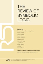
is transitive and converse well-founded. Then, a D-model is obtained by attaching infinitely many worlds
$\prec $
is transitive and converse well-founded. Then, a D-model is obtained by attaching infinitely many worlds
 $t_1, t_2, \ldots $
(called ‘tail’), and
$t_1, t_2, \ldots $
(called ‘tail’), and
 $t_\omega $
(called ‘bottom’) to a world
$t_\omega $
(called ‘bottom’) to a world
 $t_0$
of a GL-model so that
$t_0$
of a GL-model so that
 $t_0 \succ t_1 \succ t_2 \succ \cdots \succ t_\omega $
(Figure 1, Left). A non-normal modal logic
$t_0 \succ t_1 \succ t_2 \succ \cdots \succ t_\omega $
(Figure 1, Left). A non-normal modal logic
 $\mathbf {D}$
, which was studied by Beklemishev [Reference Beklemishev3], is characterized as follows. A formula
$\mathbf {D}$
, which was studied by Beklemishev [Reference Beklemishev3], is characterized as follows. A formula
 $\varphi $
is a theorem of
$\varphi $
is a theorem of
 $\mathbf {D}$
if and only if
$\mathbf {D}$
if and only if
 $\varphi $
is true at the bottom of any D-model.Footnote
1
$\varphi $
is true at the bottom of any D-model.Footnote
1

Figure 1 (Left) D-model by Beklemishev. (Right) New D-model.
 $\mathbf {D}$
is a provability logic as follows. A formula
$\mathbf {D}$
is a provability logic as follows. A formula
 $\varphi $
is a theorem of
$\varphi $
is a theorem of
 $\mathbf {D}$
if and only if any
$\mathbf {D}$
if and only if any
 $\varphi ^*$
is true in the standard model of arithmetic where
$\varphi ^*$
is true in the standard model of arithmetic where
 $\varphi ^*$
is obtained from
$\varphi ^*$
is obtained from
 $\varphi $
by interpreting the modal operator
$\varphi $
by interpreting the modal operator
 $\Box $
as the provability predicate of a c.e. extension of Peano Arithmetic that is
$\Box $
as the provability predicate of a c.e. extension of Peano Arithmetic that is
 $\Sigma _1$
-sound but not sound. In this paper, we do not argue
$\Sigma _1$
-sound but not sound. In this paper, we do not argue
 $\mathbf {D}$
from the perspective of provability logics, but we consider
$\mathbf {D}$
from the perspective of provability logics, but we consider
 $\mathbf {D}$
as an interesting modal logic which is non-normal (not closed under the necessitation rule) and has simple Kripke-style semantics. We establish sequent calculi, cut-elimination, and new Hilbert-style axiomatizations for
$\mathbf {D}$
as an interesting modal logic which is non-normal (not closed under the necessitation rule) and has simple Kripke-style semantics. We establish sequent calculi, cut-elimination, and new Hilbert-style axiomatizations for
 $\mathbf {D}$
; furthermore, we show that we can define D-models using an arbitrary limit ordinal
$\mathbf {D}$
; furthermore, we show that we can define D-models using an arbitrary limit ordinal
 $\lambda $
as well as
$\lambda $
as well as
 $\omega $
(Figure 1, Right).
$\omega $
(Figure 1, Right).
 $\mathbf {D}$
is closely related to the well-known provability logics
$\mathbf {D}$
is closely related to the well-known provability logics
 $\mathbf {GL}$
and
$\mathbf {GL}$
and
 $\mathbf {S}$
(see, e.g., [Reference Boolos5, Reference Solovay12] for the basic results on
$\mathbf {S}$
(see, e.g., [Reference Boolos5, Reference Solovay12] for the basic results on
 $\mathbf {GL}$
and
$\mathbf {GL}$
and
 $\mathbf {S}$
)Footnote
2
. A Hilbert-style proof system for
$\mathbf {S}$
)Footnote
2
. A Hilbert-style proof system for
 $\mathbf {GL}$
is known as
$\mathbf {GL}$
is known as
 $\mathbf {K} + \Box (\Box \varphi {\to } \varphi ) {\to } \Box \varphi $
. A Hilbert-style proof system for
$\mathbf {K} + \Box (\Box \varphi {\to } \varphi ) {\to } \Box \varphi $
. A Hilbert-style proof system for
 $\mathbf {S}$
(we call this system
$\mathbf {S}$
(we call this system
 ${{\mathbf {S}_{\mathrm {H}}}}$
) is as follows. The axioms are all theorems of
${{\mathbf {S}_{\mathrm {H}}}}$
) is as follows. The axioms are all theorems of
 $\mathbf {GL}$
and all formulas
$\mathbf {GL}$
and all formulas
 $\Box \varphi {\to } \varphi $
; and sole inference rule is modus ponens. Then a Hilbert-style proof system for
$\Box \varphi {\to } \varphi $
; and sole inference rule is modus ponens. Then a Hilbert-style proof system for
 $\mathbf {D}$
(we call this system
$\mathbf {D}$
(we call this system
 ${{\mathbf {D}_{\mathrm {H}}}}$
) is known to be obtained from
${{\mathbf {D}_{\mathrm {H}}}}$
) is known to be obtained from
 ${{\mathbf {S}_{\mathrm {H}}}}$
by restricting
${{\mathbf {S}_{\mathrm {H}}}}$
by restricting
 $\varphi $
in the axiom scheme
$\varphi $
in the axiom scheme
 $\Box \varphi {\to } \varphi $
to be
$\Box \varphi {\to } \varphi $
to be
 ${\bot }$
or
${\bot }$
or
 $\Box \psi {\lor } \Box \sigma $
(see [Reference Beklemishev3]). Therefore
$\Box \psi {\lor } \Box \sigma $
(see [Reference Beklemishev3]). Therefore
 $\mathbf {D}$
is an intermediate logic between
$\mathbf {D}$
is an intermediate logic between
 $\mathbf {GL}$
and
$\mathbf {GL}$
and
 $\mathbf {S}$
.
$\mathbf {S}$
.
As for sequent calculi,
 $\mathbf {GL}$
has been well studied (see, e.g., [Reference Goré and Ramanayake8] and its references), and
$\mathbf {GL}$
has been well studied (see, e.g., [Reference Goré and Ramanayake8] and its references), and
 $\mathbf {S}$
has been studied in [Reference Beklemishev2, Reference Kashima and Kato9, Reference Kushida10]. But there has been no sequent calculi for
$\mathbf {S}$
has been studied in [Reference Beklemishev2, Reference Kashima and Kato9, Reference Kushida10]. But there has been no sequent calculi for
 $\mathbf {D}$
. The sequent calculus for
$\mathbf {D}$
. The sequent calculus for
 $\mathbf {S}$
in [Reference Beklemishev2, Reference Kashima and Kato9, Reference Kushida10] was inspired by the Hilbert-style system
$\mathbf {S}$
in [Reference Beklemishev2, Reference Kashima and Kato9, Reference Kushida10] was inspired by the Hilbert-style system
 ${{\mathbf {S}_{\mathrm {H}}}}$
; so one may try to make a sequent calculus for
${{\mathbf {S}_{\mathrm {H}}}}$
; so one may try to make a sequent calculus for
 $\mathbf {D}$
based on the system
$\mathbf {D}$
based on the system
 ${{\mathbf {D}_{\mathrm {H}}}}$
. However, this attempt does not seem to work well because the axiom
${{\mathbf {D}_{\mathrm {H}}}}$
. However, this attempt does not seem to work well because the axiom
 $\Box (\Box \psi {\lor } \Box \sigma ) {\to } (\Box \psi {\lor } \Box \sigma )$
does not seem to be translatable into a rule of sequent calculi.
$\Box (\Box \psi {\lor } \Box \sigma ) {\to } (\Box \psi {\lor } \Box \sigma )$
does not seem to be translatable into a rule of sequent calculi.
In this paper, we establish sequent calculi for
 $\mathbf {D}$
so that the completeness with respect to D-models naturally holds. A key idea of our calculi is the use of three kinds of sequents. While Kushida [Reference Kushida10] used two kinds of sequents to make the calculus for
$\mathbf {D}$
so that the completeness with respect to D-models naturally holds. A key idea of our calculi is the use of three kinds of sequents. While Kushida [Reference Kushida10] used two kinds of sequents to make the calculus for
 $\mathbf {S}$
, we add one more kind. We call the three kinds ‘GL-sequents’, ‘S-sequents’, and ‘D-sequents’; these respectively correspond to the truth at the GL-model, at the tail, and at the bottom in Figure 1. Moreover, as the names suggest, these correspond to the provability of
$\mathbf {S}$
, we add one more kind. We call the three kinds ‘GL-sequents’, ‘S-sequents’, and ‘D-sequents’; these respectively correspond to the truth at the GL-model, at the tail, and at the bottom in Figure 1. Moreover, as the names suggest, these correspond to the provability of
 $\mathbf {GL}$
,
$\mathbf {GL}$
,
 $\mathbf {S}$
, and
$\mathbf {S}$
, and
 $\mathbf {D}$
, respectively.
$\mathbf {D}$
, respectively.
Strictly speaking, we give two sequent calculi, called
 ${{\mathbf {D}_{\mathrm {seq}}^{2}}}$
and
${{\mathbf {D}_{\mathrm {seq}}^{2}}}$
and
 ${{\mathbf {D}_{\mathrm {seq}}^{3}}}$
. The latter calculus
${{\mathbf {D}_{\mathrm {seq}}^{3}}}$
. The latter calculus
 ${{\mathbf {D}_{\mathrm {seq}}^{3}}}$
is cut-eliminable, and the former calculus
${{\mathbf {D}_{\mathrm {seq}}^{3}}}$
is cut-eliminable, and the former calculus
 ${{\mathbf {D}_{\mathrm {seq}}^{2}}}$
is not fully cut-eliminable but has the subformula property (we call this property ‘analytic’). We show semantic cut-elimination for both calculi (i.e., completeness of cut-free
${{\mathbf {D}_{\mathrm {seq}}^{2}}}$
is not fully cut-eliminable but has the subformula property (we call this property ‘analytic’). We show semantic cut-elimination for both calculi (i.e., completeness of cut-free
 ${{\mathbf {D}_{\mathrm {seq}}^{3}}}$
and analytic
${{\mathbf {D}_{\mathrm {seq}}^{3}}}$
and analytic
 ${{\mathbf {D}_{\mathrm {seq}}^{2}}}$
) and syntactic cut-elimination for
${{\mathbf {D}_{\mathrm {seq}}^{2}}}$
) and syntactic cut-elimination for
 ${{\mathbf {D}_{\mathrm {seq}}^{3}}}$
. These semantic arguments are extensions of that for
${{\mathbf {D}_{\mathrm {seq}}^{3}}}$
. These semantic arguments are extensions of that for
 $\mathbf {S}$
in [Reference Kashima and Kato9], and the syntactic cut-elimination is reduced to that for
$\mathbf {S}$
in [Reference Kashima and Kato9], and the syntactic cut-elimination is reduced to that for
 $\mathbf {S}$
by [Reference Kushida10].
$\mathbf {S}$
by [Reference Kushida10].
Remark 1.1. A proof in
 ${{\mathbf {D}_{\mathrm {seq}}^{3}}}$
has three layers with three kinds of sequents, and the syntactic cut-elimination for the bottom layer (with D-sequents) is reduced to that for the middle layer (with S-sequents). Similar arguments—a proof has layered structure and the cut-elimination for the lower layer is reduced to that for the upper layer—are found in [Reference Lang, Ramanayake and Urban11].
${{\mathbf {D}_{\mathrm {seq}}^{3}}}$
has three layers with three kinds of sequents, and the syntactic cut-elimination for the bottom layer (with D-sequents) is reduced to that for the middle layer (with S-sequents). Similar arguments—a proof has layered structure and the cut-elimination for the lower layer is reduced to that for the upper layer—are found in [Reference Lang, Ramanayake and Urban11].
Then, two new Hilbert-style proof systems (we call these
 ${{\mathbf {D}_{\mathrm {H}}^{2}}}$
and
${{\mathbf {D}_{\mathrm {H}}^{2}}}$
and
 ${{\mathbf {D}_{\mathrm {H}}^{3}}}$
) for
${{\mathbf {D}_{\mathrm {H}}^{3}}}$
) for
 $\mathbf {D}$
are obtained by interpreting the sequent calculi
$\mathbf {D}$
are obtained by interpreting the sequent calculi
 ${{\mathbf {D}_{\mathrm {seq}}^{2}}}$
and
${{\mathbf {D}_{\mathrm {seq}}^{2}}}$
and
 ${{\mathbf {D}_{\mathrm {seq}}^{3}}}$
, respectively. Here, not only the existing system
${{\mathbf {D}_{\mathrm {seq}}^{3}}}$
, respectively. Here, not only the existing system
 ${{\mathbf {D}_{\mathrm {H}}}}$
but also the new systems
${{\mathbf {D}_{\mathrm {H}}}}$
but also the new systems
 ${{\mathbf {D}_{\mathrm {H}}^{2}}}$
and
${{\mathbf {D}_{\mathrm {H}}^{2}}}$
and
 ${{\mathbf {D}_{\mathrm {H}}^{3}}}$
have ‘all theorems of
${{\mathbf {D}_{\mathrm {H}}^{3}}}$
have ‘all theorems of
 $\mathbf {GL}$
’ as their axioms; so it is natural to argue a generalization as follows. Let L be an arbitrary modal logic, and let
$\mathbf {GL}$
’ as their axioms; so it is natural to argue a generalization as follows. Let L be an arbitrary modal logic, and let
 ${{\mathbf {D}_{\mathrm {H}}[L]}}$
,
${{\mathbf {D}_{\mathrm {H}}[L]}}$
,
 ${{\mathbf {D}_{\mathrm {H}}^{2}[L]}}$
, and
${{\mathbf {D}_{\mathrm {H}}^{2}[L]}}$
, and
 ${{\mathbf {D}_{\mathrm {H}}^{3}[L]}}$
be the Hilbert-style systems obtained from
${{\mathbf {D}_{\mathrm {H}}^{3}[L]}}$
be the Hilbert-style systems obtained from
 ${{\mathbf {D}_{\mathrm {H}}}}$
,
${{\mathbf {D}_{\mathrm {H}}}}$
,
 ${{\mathbf {D}_{\mathrm {H}}^{2}}}$
, and
${{\mathbf {D}_{\mathrm {H}}^{2}}}$
, and
 ${{\mathbf {D}_{\mathrm {H}}^{3}}}$
, respectively, by replacing the axioms ‘theorems of
${{\mathbf {D}_{\mathrm {H}}^{3}}}$
, respectively, by replacing the axioms ‘theorems of
 $\mathbf {GL}$
’ with ‘theorems of L’. On the other hand, let
$\mathbf {GL}$
’ with ‘theorems of L’. On the other hand, let
 ${\cal F}$
be a class of Kripke frames, and let ‘
${\cal F}$
be a class of Kripke frames, and let ‘
 $\mathbf {D}[{\cal F}]$
-model’ denote any Kripke model described as Figure 1 in which ‘GL-model’ is replaced with ‘
$\mathbf {D}[{\cal F}]$
-model’ denote any Kripke model described as Figure 1 in which ‘GL-model’ is replaced with ‘
 ${\cal F}$
-model’. Then we show the following:
${\cal F}$
-model’. Then we show the following:
If L is characterized by
 ${\cal F}$
and if a certain condition is satisfied, then the following conditions are equivalent: (1)
${\cal F}$
and if a certain condition is satisfied, then the following conditions are equivalent: (1)
 $\varphi $
is true at the bottom of any
$\varphi $
is true at the bottom of any
 $\mathbf {D}[{\cal F}]$
-model. (2)
$\mathbf {D}[{\cal F}]$
-model. (2)
 $\varphi $
is a theorem of
$\varphi $
is a theorem of
 ${\mathbf {D}_{\mathrm {H}}^{2}[L]}$
. (3)
${\mathbf {D}_{\mathrm {H}}^{2}[L]}$
. (3)
 $\varphi $
is a theorem of
$\varphi $
is a theorem of
 ${\mathbf {D}_{\mathrm {H}}^{3}[L]}$
.
${\mathbf {D}_{\mathrm {H}}^{3}[L]}$
.
This statement is just the completeness theorem of
 ${{\mathbf {D}_{\mathrm {H}}^{2}}}$
and
${{\mathbf {D}_{\mathrm {H}}^{2}}}$
and
 ${{\mathbf {D}_{\mathrm {H}}^{3}}}$
if
${{\mathbf {D}_{\mathrm {H}}^{3}}}$
if
 $L = \mathbf {GL}$
and
$L = \mathbf {GL}$
and
 ${\cal F}$
is the class of transitive and converse well-founded frames. It seems that the condition ‘
${\cal F}$
is the class of transitive and converse well-founded frames. It seems that the condition ‘
 $\varphi $
is a theorem of
$\varphi $
is a theorem of
 ${\mathbf {D}_{\mathrm {H}}[L]}$
’ is not equivalent to the above three conditions. This fact shows that the new proof systems—
${\mathbf {D}_{\mathrm {H}}[L]}$
’ is not equivalent to the above three conditions. This fact shows that the new proof systems—
 ${{\mathbf {D}_{\mathrm {H}}^{2}}}$
,
${{\mathbf {D}_{\mathrm {H}}^{2}}}$
,
 ${{\mathbf {D}_{\mathrm {H}}^{3}}}$
, and the two sequent calculi—well reflect the essence of the modal logic
${{\mathbf {D}_{\mathrm {H}}^{3}}}$
, and the two sequent calculi—well reflect the essence of the modal logic
 $\mathbf {D}$
, and that the new systems are more natural than the existing system
$\mathbf {D}$
, and that the new systems are more natural than the existing system
 ${{\mathbf {D}_{\mathrm {H}}}}$
.
${{\mathbf {D}_{\mathrm {H}}}}$
.
The structure of this paper is as follows. In Section 2, we present results that are known or will be shown in later sections. In Section 3, we recall the sequent calculi for
 $\mathbf {GL}$
and
$\mathbf {GL}$
and
 $\mathbf {S}$
, and we introduce two sequent calculi
$\mathbf {S}$
, and we introduce two sequent calculi
 ${{\mathbf {D}_{\mathrm {seq}}^{2}}}$
and
${{\mathbf {D}_{\mathrm {seq}}^{2}}}$
and
 ${{\mathbf {D}_{\mathrm {seq}}^{3}}}$
. In Section 4, we give syntactic arguments on the sequent calculi. In Section 5, we show the semantic cut-elimination. In Section 6, we introduce Hilbert-style systems
${{\mathbf {D}_{\mathrm {seq}}^{3}}}$
. In Section 4, we give syntactic arguments on the sequent calculi. In Section 5, we show the semantic cut-elimination. In Section 6, we introduce Hilbert-style systems
 ${{\mathbf {D}_{\mathrm {H}}^{2}}}$
and
${{\mathbf {D}_{\mathrm {H}}^{2}}}$
and
 ${{\mathbf {D}_{\mathrm {H}}^{3}}}$
. In Section 7, we show the general result on
${{\mathbf {D}_{\mathrm {H}}^{3}}}$
. In Section 7, we show the general result on
 ${\mathbf {D}_{\mathrm {H}}^{2}[L]}$
and
${\mathbf {D}_{\mathrm {H}}^{2}[L]}$
and
 ${\mathbf {D}_{\mathrm {H}}^{3}[L]}$
.
${\mathbf {D}_{\mathrm {H}}^{3}[L]}$
.
2 Preliminaries and results
Formulas are constructed from propositional variables, propositional constant
 ${\bot }$
, logical operator
${\bot }$
, logical operator
 ${\to }$
, and modal operator
${\to }$
, and modal operator
 $\Box $
. The other operators are defined as abbreviations as usual. The letters
$\Box $
. The other operators are defined as abbreviations as usual. The letters
 $p, q, \ldots $
denote propositional variables and the letters
$p, q, \ldots $
denote propositional variables and the letters
 $\varphi , \psi , \ldots $
denote formulas. The set of propositional variables is called PropVar and the set of formulas is called
$\varphi , \psi , \ldots $
denote formulas. The set of propositional variables is called PropVar and the set of formulas is called
 ${\mathbf {Form}}$
. Parentheses are omitted as, for example,
${\mathbf {Form}}$
. Parentheses are omitted as, for example,
 $\Box \varphi {\land } \psi {\to } \Box \pi {\lor } \sigma = ((\Box \varphi ) {\land } \psi ) {\to } ((\Box \pi ) {\lor } \sigma )$
.
$\Box \varphi {\land } \psi {\to } \Box \pi {\lor } \sigma = ((\Box \varphi ) {\land } \psi ) {\to } ((\Box \pi ) {\lor } \sigma )$
.
Hilbert-style proof systems
 ${{\mathbf {GL}_{\mathrm {H}}}}$
,
${{\mathbf {GL}_{\mathrm {H}}}}$
,
 ${{\mathbf {S}_{\mathrm {H}}}}$
, and
${{\mathbf {S}_{\mathrm {H}}}}$
, and
 ${{\mathbf {D}_{\mathrm {H}}}}$
are known as follows, where the subscript H denotes ‘Hilbert-style’.
${{\mathbf {D}_{\mathrm {H}}}}$
are known as follows, where the subscript H denotes ‘Hilbert-style’.
Axioms of
 ${{\mathbf {GL}_{\mathrm {H}}}}$
: Tautologies,
${{\mathbf {GL}_{\mathrm {H}}}}$
: Tautologies,
 $\Box (\varphi {\to } \psi ) {\to } (\Box \varphi {\to } \Box \psi )$
, and
$\Box (\varphi {\to } \psi ) {\to } (\Box \varphi {\to } \Box \psi )$
, and
 $\Box (\Box \varphi {\to } \varphi ) {\to } \Box \varphi $
.
$\Box (\Box \varphi {\to } \varphi ) {\to } \Box \varphi $
.
Rules of
 ${{\mathbf {GL}_{\mathrm {H}}}}$
:
${{\mathbf {GL}_{\mathrm {H}}}}$
: ![]()
Axioms of
 ${{\mathbf {S}_{\mathrm {H}}}}$
: Theorems of
${{\mathbf {S}_{\mathrm {H}}}}$
: Theorems of
 ${{\mathbf {GL}_{\mathrm {H}}}}$
and
${{\mathbf {GL}_{\mathrm {H}}}}$
and
 $\Box \varphi {\to } \varphi $
.
$\Box \varphi {\to } \varphi $
.
Rule of
 ${{\mathbf {S}_{\mathrm {H}}}}$
: Modus ponens.
${{\mathbf {S}_{\mathrm {H}}}}$
: Modus ponens.
Axioms of
 ${{\mathbf {D}_{\mathrm {H}}}}$
: Theorems of
${{\mathbf {D}_{\mathrm {H}}}}$
: Theorems of
 ${\mathbf {GL}_{\mathrm {H}}}$
,
${\mathbf {GL}_{\mathrm {H}}}$
,
 ${\lnot }\Box {\bot }$
, and
${\lnot }\Box {\bot }$
, and
 $\Box (\Box \varphi {\lor } \Box \psi ) {\to } \Box \varphi {\lor } \Box \psi $
.
$\Box (\Box \varphi {\lor } \Box \psi ) {\to } \Box \varphi {\lor } \Box \psi $
.
Rule of
 ${{\mathbf {D}_{\mathrm {H}}}}$
: Modus ponens.
${{\mathbf {D}_{\mathrm {H}}}}$
: Modus ponens.
The symbol
 $\vdash $
denotes provability as usual. We have
$\vdash $
denotes provability as usual. We have
 $ ({{\mathbf {GL}_{\mathrm {H}}}} \vdash \varphi ) \Longrightarrow ({{\mathbf {D}_{\mathrm {H}}}} \vdash \varphi ) \Longrightarrow ({{\mathbf {S}_{\mathrm {H}}}} \vdash \varphi )$
, but the converse does not hold in general; for example,
$ ({{\mathbf {GL}_{\mathrm {H}}}} \vdash \varphi ) \Longrightarrow ({{\mathbf {D}_{\mathrm {H}}}} \vdash \varphi ) \Longrightarrow ({{\mathbf {S}_{\mathrm {H}}}} \vdash \varphi )$
, but the converse does not hold in general; for example,
 $\Box p {\to } p$
is provable in
$\Box p {\to } p$
is provable in
 ${{\mathbf {S}_{\mathrm {H}}}}$
but not provable in
${{\mathbf {S}_{\mathrm {H}}}}$
but not provable in
 ${{\mathbf {D}_{\mathrm {H}}}}$
. Note that neither
${{\mathbf {D}_{\mathrm {H}}}}$
. Note that neither
 ${{\mathbf {D}_{\mathrm {H}}}}$
nor
${{\mathbf {D}_{\mathrm {H}}}}$
nor
 ${{\mathbf {S}_{\mathrm {H}}}}$
has the inference rule (
${{\mathbf {S}_{\mathrm {H}}}}$
has the inference rule (
 $\Box $
). For example, we have
$\Box $
). For example, we have
 ${{\mathbf {D}_{\mathrm {H}}}} \vdash {\lnot }\Box {\bot }$
but
${{\mathbf {D}_{\mathrm {H}}}} \vdash {\lnot }\Box {\bot }$
but
 ${{\mathbf {D}_{\mathrm {H}}}} \not \vdash \Box {\lnot }\Box {\bot }$
.
${{\mathbf {D}_{\mathrm {H}}}} \not \vdash \Box {\lnot }\Box {\bot }$
.
A Kripke model
 $\langle W, \prec , V\rangle $
consists of a non-empty set W of worlds, an accessibility relation
$\langle W, \prec , V\rangle $
consists of a non-empty set W of worlds, an accessibility relation
 ${\prec } \subseteq W \times W$
, and a valuation
${\prec } \subseteq W \times W$
, and a valuation
 $V: W \times {\mathbf {PropVar}} \to \{\mathsf {true}, \mathsf {false}\}$
. The domain of V is extended to
$V: W \times {\mathbf {PropVar}} \to \{\mathsf {true}, \mathsf {false}\}$
. The domain of V is extended to
 $W \times {\mathbf {Form}}$
by the following:
$W \times {\mathbf {Form}}$
by the following:
 $V(w,{\bot }) = \mathsf {false}$
.
$V(w,{\bot }) = \mathsf {false}$
.
 $V(w, \varphi {\to }\psi ) = \mathsf {true} \Longleftrightarrow V(w, \varphi ) = \mathsf {false} \text { or } V(w, \psi ) = \mathsf {true}.$
 $V(w,\Box \varphi ) = \mathsf {true} \Longleftrightarrow (\forall w' \succ w)(V(w',\varphi ) = \mathsf {true}).$
 $\langle W, \prec \rangle $
is called the Kripke frame of this model, and
$\langle W, \prec \rangle $
is called the Kripke frame of this model, and
 $\langle W, \prec , V\rangle $
is called a Kripke model based on the frame
$\langle W, \prec , V\rangle $
is called a Kripke model based on the frame
 $\langle W, \prec \rangle $
. We say that a formula
$\langle W, \prec \rangle $
. We say that a formula
 $\varphi $
is true at a world w if
$\varphi $
is true at a world w if
 $V(w,\varphi ) = \mathsf {true}$
.
$V(w,\varphi ) = \mathsf {true}$
.
A Kripke frame
 $\langle W, \prec \rangle $
is called a GL-frame if
$\langle W, \prec \rangle $
is called a GL-frame if
 ${\prec }$
is converse well-founded (i.e., there is no infinitely ascending sequence
${\prec }$
is converse well-founded (i.e., there is no infinitely ascending sequence
 $x_1 \prec x_2 \prec x_3 \cdots $
) and transitive. A Kripke model based on a GL-frame is called a GL-model. The completeness of
$x_1 \prec x_2 \prec x_3 \cdots $
) and transitive. A Kripke model based on a GL-frame is called a GL-model. The completeness of
 ${{\mathbf {GL}_{\mathrm {H}}}}$
is well-known as below (see, e.g., [Reference Boolos5]).
${{\mathbf {GL}_{\mathrm {H}}}}$
is well-known as below (see, e.g., [Reference Boolos5]).
Proposition 2.1 (Completeness of
 ${{\mathbf {GL}_{\mathrm {H}}}}$
).
${{\mathbf {GL}_{\mathrm {H}}}}$
).

The following are equivalent:
-
•
${\mathbf {GL}_{\mathrm {H}}} \vdash \varphi $
. -
•
$\varphi $
is true at any world of any GL-model.


To describe the semantics for
 ${{\mathbf {S}_{\mathrm {H}}}}$
and
${{\mathbf {S}_{\mathrm {H}}}}$
and
 ${{\mathbf {D}_{\mathrm {H}}}}$
, we need further definitions.
${{\mathbf {D}_{\mathrm {H}}}}$
, we need further definitions.
Definition 2.2. Let
 $\lambda $
be a limit ordinal. We say that a frame
$\lambda $
be a limit ordinal. We say that a frame
 $\langle W^+, \prec ^+\rangle $
is a
$\langle W^+, \prec ^+\rangle $
is a
 $\lambda $
-extension of
$\lambda $
-extension of
 $\langle W, \prec \rangle $
if the following two conditions hold for some
$\langle W, \prec \rangle $
if the following two conditions hold for some
 $t_0 \in W$
.
$t_0 \in W$
.
 $W^+ = W \uplus \{t_\alpha \mid 0 < \alpha \leq \lambda \}$
.
$W^+ = W \uplus \{t_\alpha \mid 0 < \alpha \leq \lambda \}$
.
 ${\prec }^+ = {\prec } \cup \{(t_{\alpha }, t_{\beta }) \mid 0 \leq \beta < \alpha \leq \lambda \} \cup \{(t_{\alpha }, x) \mid 0 < \alpha \leq \lambda \text { and } (t_{0}, x) \in {\prec }\}.$
(Refer to Figure 1, in which the ellipse is
 $\langle W, \prec \rangle $
.) The infinite set
$\langle W, \prec \rangle $
.) The infinite set
 $\{t_\alpha \mid 0 < \alpha < \lambda \}$
is called the tail and the world
$\{t_\alpha \mid 0 < \alpha < \lambda \}$
is called the tail and the world
 $t_\lambda $
is called the bottom of this frame. If a valuation
$t_\lambda $
is called the bottom of this frame. If a valuation
 $V^+$
coincides with V for any worlds in W, then we say that the Kripke model
$V^+$
coincides with V for any worlds in W, then we say that the Kripke model
 $M^+ = \langle W^+, \prec ^+, V^+\rangle $
is a
$M^+ = \langle W^+, \prec ^+, V^+\rangle $
is a
 $\lambda $
-extension of
$\lambda $
-extension of
 $M = \langle W, \prec , V\rangle $
. Moreover,
$M = \langle W, \prec , V\rangle $
. Moreover,
 $M^+$
is called a constant or a strongly constant
$M^+$
is called a constant or a strongly constant
 $\lambda $
-extension of M if the following condition holds, respectively.
$\lambda $
-extension of M if the following condition holds, respectively.

We say that a formula
 $\varphi $
is eventually always true in the tail of
$\varphi $
is eventually always true in the tail of
 $M^+$
if
$M^+$
if
 $(\exists \alpha <\lambda )(\alpha < \forall \beta < \lambda )(V(t_\beta , \varphi ) = \mathsf {true})$
.
$(\exists \alpha <\lambda )(\alpha < \forall \beta < \lambda )(V(t_\beta , \varphi ) = \mathsf {true})$
.
The following proposition is easy to be proved. This will be used implicitly in this paper.
Proposition 2.3. If
 $\langle W^+, \prec ^+, V^+\rangle $
is a
$\langle W^+, \prec ^+, V^+\rangle $
is a
 $\lambda $
-extension of
$\lambda $
-extension of
 $\langle W, \prec , V\rangle $
, then for any world
$\langle W, \prec , V\rangle $
, then for any world
 $w \in W$
and any formula
$w \in W$
and any formula
 $\varphi $
, we have
$\varphi $
, we have
 $V^+(w, \varphi ) = V(w, \varphi )$
.
$V^+(w, \varphi ) = V(w, \varphi )$
.
The completeness of
 ${{\mathbf {S}_{\mathrm {H}}}}$
is described below, which will be proved in Section 5.
${{\mathbf {S}_{\mathrm {H}}}}$
is described below, which will be proved in Section 5.
Proposition 2.4 (Completeness of
${{\mathbf {S}_{\mathrm {H}}}}$
).

Let
 $\lambda $
be a limit ordinal. The following are equivalent:
$\lambda $
be a limit ordinal. The following are equivalent:
-
(s1)
${\mathbf {S}_{\mathrm {H}}} \vdash \varphi $
. -
(s2)
$\varphi $
is true at the bottom of any strongly constant
$\lambda $
-extension of any GL-model. -
(s3)
$\varphi $
is eventually always true in the tail of any (strongly) constant
$\lambda $
-extension of any GL-model. -
(s4)
$\varphi $
is eventually always true in the tail of any
$\lambda $
-extension of any GL-model.


Remark 2.5. The completeness of
 ${{\mathbf {S}_{\mathrm {H}}}}$
has been expressed in several different statements in [Reference Beklemishev3, Reference Boolos4, Reference Chagrov and Zakharyaschev6, Reference Kashima and Kato9, Reference Visser14], but all of them are essentially included in the
${{\mathbf {S}_{\mathrm {H}}}}$
has been expressed in several different statements in [Reference Beklemishev3, Reference Boolos4, Reference Chagrov and Zakharyaschev6, Reference Kashima and Kato9, Reference Visser14], but all of them are essentially included in the
 $\lambda = \omega $
case of Proposition 2.4. In this paper, we extend it to arbitrary limit ordinals.
$\lambda = \omega $
case of Proposition 2.4. In this paper, we extend it to arbitrary limit ordinals.
Remark 2.6. The limit ordinal
 $\lambda $
is arbitrarily fixed at the beginning of Proposition 2.4. On the other hand, we can consider propositions in which
$\lambda $
is arbitrarily fixed at the beginning of Proposition 2.4. On the other hand, we can consider propositions in which
 $\lambda $
is bound at each sentence; for example, there are two variants of the condition (s2) as follows:
$\lambda $
is bound at each sentence; for example, there are two variants of the condition (s2) as follows:
(s2
 $^+$
)
$^+$
)
 $\varphi $
is true at the bottom of any strongly constant
$\varphi $
is true at the bottom of any strongly constant
 $\lambda '$
-extension of any GL-model, for any limit ordinal
$\lambda '$
-extension of any GL-model, for any limit ordinal
 $\lambda '$
.
$\lambda '$
.
(s2
 $^-$
)
$^-$
)
 $\varphi $
is true at the bottom of any strongly constant
$\varphi $
is true at the bottom of any strongly constant
 $\lambda '$
-extension of any GL-model, for some limit ordinal
$\lambda '$
-extension of any GL-model, for some limit ordinal
 $\lambda '$
.
$\lambda '$
.
The conditions (s2
 $^+$
), (s2
$^+$
), (s2
 $^-$
), and (s2) are equivalent for any
$^-$
), and (s2) are equivalent for any
 $\lambda $
, because we have the following implications.
$\lambda $
, because we have the following implications.
 $$\begin{align*}(\mathrm{s2}^+) \ \stackrel{}{\Longrightarrow} \ (\mathrm{s2}^-) \ \stackrel{\text{Prop}~2.4}{\Longrightarrow} \ (\mathrm{s1}) \ \stackrel{\text{Prop}~2.4}{\Longrightarrow} \ (\mathrm{s2}^+). \end{align*}$$
So, from now on, we will not mention conditions like (s2
 $^+$
) or (s2
$^+$
) or (s2
 $^-$
) (except for a condition in Theorem 7.7).
$^-$
) (except for a condition in Theorem 7.7).
The completeness of
 ${{\mathbf {D}_{\mathrm {H}}}}$
is described below, which will be proved in Sections 5 and 6.
${{\mathbf {D}_{\mathrm {H}}}}$
is described below, which will be proved in Sections 5 and 6.
Proposition 2.7 (Completeness of
${{\mathbf {D}_{\mathrm {H}}}}$
).

Let
 $\lambda $
be a limit ordinal. The following are equivalent:
$\lambda $
be a limit ordinal. The following are equivalent:
-
(d1)
${\mathbf {D}_{\mathrm {H}}} \vdash \varphi $
. -
(d2)
$\varphi $
is true at the bottom of any constant
$\lambda $
-extension of any GL-model. -
(d3)
$\varphi $
is true at the bottom of any
$\lambda $
-extension of any GL-model.


Remark 2.8. Beklemishev [Reference Beklemishev3] proved the equivalence between (d1), (d2) for
 $\lambda = \omega $
, and another condition using ‘accumulating root’. In Section 5, we will show the equivalence between (d2) and (d3). In Section 6, we will show the equivalence between (d1) and others.
$\lambda = \omega $
, and another condition using ‘accumulating root’. In Section 5, we will show the equivalence between (d2) and (d3). In Section 6, we will show the equivalence between (d1) and others.
3 Sequent calculi
We introduce sequent calculi. From now on, letters
 ${\mit \Gamma }, {\mit \Delta }, \ldots $
denote finite sets of formulas. As usual, the expression ‘
${\mit \Gamma }, {\mit \Delta }, \ldots $
denote finite sets of formulas. As usual, the expression ‘
 ${\mit \Gamma }, \varphi , \psi , {\mit \Delta }$
’, for example, stands for the set
${\mit \Gamma }, \varphi , \psi , {\mit \Delta }$
’, for example, stands for the set
 ${\mit \Gamma } \cup \{\varphi , \psi \} \cup {\mit \Delta }$
, and ‘
${\mit \Gamma } \cup \{\varphi , \psi \} \cup {\mit \Delta }$
, and ‘
 $\Box {\mit \Gamma }$
’ stands for the set
$\Box {\mit \Gamma }$
’ stands for the set
 $\{\Box \gamma \mid \gamma \in {\mit \Gamma }\}$
.
$\{\Box \gamma \mid \gamma \in {\mit \Gamma }\}$
.
 $\mathrm {Sub}({\mit \Gamma })$
denotes the set of all subformulas of formulas in
$\mathrm {Sub}({\mit \Gamma })$
denotes the set of all subformulas of formulas in
 ${\mit \Gamma }$
.
${\mit \Gamma }$
.
We use three different arrows
 $\Rightarrow $
,
$\Rightarrow $
,
 $\Rrightarrow $
, and
$\Rrightarrow $
, and
 $\Rightarrow \!\!\!\!\Rightarrow $
to define three kinds of sequents
$\Rightarrow \!\!\!\!\Rightarrow $
to define three kinds of sequents
 ${{\mit \Gamma }}\Rightarrow {{\mit \Delta }}$
(called GL-sequent),
${{\mit \Gamma }}\Rightarrow {{\mit \Delta }}$
(called GL-sequent),
 ${{\mit \Gamma }}\Rrightarrow {{\mit \Delta }}$
(called S-sequent), and
${{\mit \Gamma }}\Rrightarrow {{\mit \Delta }}$
(called S-sequent), and
 ${{\mit \Gamma }}\Rightarrow \!\!\!\!\Rightarrow {{\mit \Delta }}$
(called D-sequent).
${{\mit \Gamma }}\Rightarrow \!\!\!\!\Rightarrow {{\mit \Delta }}$
(called D-sequent).
The following is the well-known sequent calculus for classical propositional logic; we call it
 ${{\mathbf {LK}_{\Rightarrow }}}$
.
${{\mathbf {LK}_{\Rightarrow }}}$
.
Initial sequents:
 ${\varphi }\Rightarrow {\varphi }$
and
${\varphi }\Rightarrow {\varphi }$
and
 ${{\bot }}\Rightarrow {}$
Inference rules:
Similarly the sequent calculus
 ${{\mathbf {LK}_{\Rrightarrow }}}$
(or
${{\mathbf {LK}_{\Rrightarrow }}}$
(or
 ${{\mathbf {LK}_{\Rightarrow \!\!\!\!\Rightarrow }}}$
, respectively) consists of the above initial sequents and inference rules where all ‘
${{\mathbf {LK}_{\Rightarrow \!\!\!\!\Rightarrow }}}$
, respectively) consists of the above initial sequents and inference rules where all ‘
 $\Rightarrow $
’ are replaced with ‘
$\Rightarrow $
’ are replaced with ‘
 $\Rrightarrow $
’ (or ‘
$\Rrightarrow $
’ (or ‘
 $\Rightarrow \!\!\!\!\Rightarrow $
’, respectively). Next we introduce five rules
$\Rightarrow \!\!\!\!\Rightarrow $
’, respectively). Next we introduce five rules
 $({{\text {GL}\Box }})$
,
$({{\text {GL}\Box }})$
,
 $({{\text {GLtoS}}})$
,
$({{\text {GLtoS}}})$
,
 $({\text {S}{\Box }\text {left}})$
,
$({\text {S}{\Box }\text {left}})$
,
 $({{\text {GLtoD}}})$
, and
$({{\text {GLtoD}}})$
, and
 $({{\text {StoD}}})$
as below
$({{\text {StoD}}})$
as below
Using these, we define four sequent calculi
 ${{\mathbf {GL}_{\mathrm {seq}}}}$
,
${{\mathbf {GL}_{\mathrm {seq}}}}$
,
 ${{\mathbf {S}_{\mathrm {seq}}}}$
,
${{\mathbf {S}_{\mathrm {seq}}}}$
,
 ${{\mathbf {D}_{\mathrm {seq}}^{2}}}$
, and
${{\mathbf {D}_{\mathrm {seq}}^{2}}}$
, and
 ${{\mathbf {D}_{\mathrm {seq}}^{3}}}$
according to Table 1.
${{\mathbf {D}_{\mathrm {seq}}^{3}}}$
according to Table 1.
 ${{\mathbf {GL}_{\mathrm {seq}}}}$
(
${{\mathbf {GL}_{\mathrm {seq}}}}$
(
 $ = {{\mathbf {LK}_{\Rightarrow }}} + ({\text {GL}\Box })$
) is a well-known sequent calculus for
$ = {{\mathbf {LK}_{\Rightarrow }}} + ({\text {GL}\Box })$
) is a well-known sequent calculus for
 $\mathbf {GL}$
, and has been widely studied; see [Reference Goré and Ramanayake8] and its references.
$\mathbf {GL}$
, and has been widely studied; see [Reference Goré and Ramanayake8] and its references.
 ${{\mathbf {S}_{\mathrm {seq}}}}$
(
${{\mathbf {S}_{\mathrm {seq}}}}$
(
 $ = {{\mathbf {GL}_{\mathrm {seq}}}} + ({\text {GLtoS}}) + ({\text {S}{\Box }\text {left}}) + {{\mathbf {LK}_{\Rrightarrow }}}$
) is a sequent calculus for
$ = {{\mathbf {GL}_{\mathrm {seq}}}} + ({\text {GLtoS}}) + ({\text {S}{\Box }\text {left}}) + {{\mathbf {LK}_{\Rrightarrow }}}$
) is a sequent calculus for
 $\mathbf {S}$
using two kinds of sequents (GL- and S-sequents), and it (or similar calculi) has been studied in [Reference Beklemishev2, Reference Kashima and Kato9, Reference Kushida10]. The two calculi
$\mathbf {S}$
using two kinds of sequents (GL- and S-sequents), and it (or similar calculi) has been studied in [Reference Beklemishev2, Reference Kashima and Kato9, Reference Kushida10]. The two calculi
 ${{\mathbf {D}_{\mathrm {seq}}^{2}}}$
and
${{\mathbf {D}_{\mathrm {seq}}^{2}}}$
and
 ${{\mathbf {D}_{\mathrm {seq}}^{3}}}$
are new, and they are obtained as below
${{\mathbf {D}_{\mathrm {seq}}^{3}}}$
are new, and they are obtained as below
 $$\begin{align*}{{\mathbf{D}_{\mathrm{seq}}^{2}}} = {{\mathbf{GL}_{\mathrm{seq}}}} + ({\text{GLtoD}}) + {{\mathbf{LK}_{\Rightarrow\!\!\!\!\Rightarrow}}}. \end{align*}$$
 $$\begin{align*}{{\mathbf{D}_{\mathrm{seq}}^{3}}} = {{\mathbf{S}_{\mathrm{seq}}}} + ({\text{StoD}}) + {{\mathbf{LK}_{\Rightarrow\!\!\!\!\Rightarrow}}}. \end{align*}$$
The superscripts ‘2’ and ‘3’ denote the number of kinds of sequents; that is,
 ${{\mathbf {D}_{\mathrm {seq}}^{2}}}$
uses two kinds (GL- and D-sequents) and
${{\mathbf {D}_{\mathrm {seq}}^{2}}}$
uses two kinds (GL- and D-sequents) and
 ${{\mathbf {D}_{\mathrm {seq}}^{3}}}$
uses three kinds of sequents.
${{\mathbf {D}_{\mathrm {seq}}^{3}}}$
uses three kinds of sequents.
Table 1 Four sequent calculi

Proofs in each calculus are called
 ${{\mathbf {GL}_{\mathrm {seq}}}}/{{\mathbf {S}_{\mathrm {seq}}}}/{{\mathbf {D}_{\mathrm {seq}}^{2}}}/{{\mathbf {D}_{\mathrm {seq}}^{3}}}$
-proofs. In general, an
${{\mathbf {GL}_{\mathrm {seq}}}}/{{\mathbf {S}_{\mathrm {seq}}}}/{{\mathbf {D}_{\mathrm {seq}}^{2}}}/{{\mathbf {D}_{\mathrm {seq}}^{3}}}$
-proofs. In general, an
 ${{\mathbf {S}_{\mathrm {seq}}}}$
-proof has two-layered structure (the upper layer consists of GL-sequents and the lower layer consists of S-sequents). Similarly, a
${{\mathbf {S}_{\mathrm {seq}}}}$
-proof has two-layered structure (the upper layer consists of GL-sequents and the lower layer consists of S-sequents). Similarly, a
 ${{\mathbf {D}_{\mathrm {seq}}^{2}}}$
-proof has two layers (upper: GL-sequents; lower: D-sequents), and a
${{\mathbf {D}_{\mathrm {seq}}^{2}}}$
-proof has two layers (upper: GL-sequents; lower: D-sequents), and a
 ${{\mathbf {D}_{\mathrm {seq}}^{3}}}$
-proof has three layers (top: GL-sequents; middle: S-sequents; bottom: D-sequents). Note that only
${{\mathbf {D}_{\mathrm {seq}}^{3}}}$
-proof has three layers (top: GL-sequents; middle: S-sequents; bottom: D-sequents). Note that only
 ${{\mathbf {LK}_{\Rightarrow \!\!\!\!\Rightarrow }}}$
-rules can have D-sequents as assumptions. Therefore the bottom layer of a
${{\mathbf {LK}_{\Rightarrow \!\!\!\!\Rightarrow }}}$
-rules can have D-sequents as assumptions. Therefore the bottom layer of a
 ${{\mathbf {D}_{\mathrm {seq}}^{2}}}/{{\mathbf {D}_{\mathrm {seq}}^{3}}}$
-proof consists of only
${{\mathbf {D}_{\mathrm {seq}}^{2}}}/{{\mathbf {D}_{\mathrm {seq}}^{3}}}$
-proof consists of only
 ${{\mathbf {LK}_{\Rightarrow \!\!\!\!\Rightarrow }}}$
-rules.
${{\mathbf {LK}_{\Rightarrow \!\!\!\!\Rightarrow }}}$
-rules.
As usual, the term ‘cut-free’ means ‘without using the cut rule’. The following examples are cut-free
 ${{\mathbf {D}_{\mathrm {seq}}^{2}}}/{{\mathbf {D}_{\mathrm {seq}}^{3}}}$
-proofs, where ‘w.’ stands for ‘weakening’, and (
${{\mathbf {D}_{\mathrm {seq}}^{2}}}/{{\mathbf {D}_{\mathrm {seq}}^{3}}}$
-proofs, where ‘w.’ stands for ‘weakening’, and (
 ${\lor }$
left), (
${\lor }$
left), (
 ${\lor }$
right), and (
${\lor }$
right), and (
 ${\lnot }$
right) are suitable combinations of rules in LK (since
${\lnot }$
right) are suitable combinations of rules in LK (since
 ${\lor }$
and
${\lor }$
and
 ${\lnot }$
are abbreviations).
${\lnot }$
are abbreviations).
Example 3.1.
 $\text {Cut-free}\ {\mathbf {D}_{\mathrm {seq}}^{2}} \vdash {{}\Rightarrow \!\!\!\!\Rightarrow {\Box (\Box \varphi {\lor } \Box \psi ) {\to } \Box \varphi {\lor } \Box \psi }}$
.
$\text {Cut-free}\ {\mathbf {D}_{\mathrm {seq}}^{2}} \vdash {{}\Rightarrow \!\!\!\!\Rightarrow {\Box (\Box \varphi {\lor } \Box \psi ) {\to } \Box \varphi {\lor } \Box \psi }}$
.

Example 3.2.
 $\text {Cut-free}\ {\mathbf {D}_{\mathrm {seq}}^{3}} \vdash {{}\Rightarrow \!\!\!\!\Rightarrow {\Box (\Box \varphi {\lor } \Box \psi ) {\to } \Box \varphi {\lor } \Box \psi }}.$

Example 3.3.
 $\text {Cut-free}\ {\mathbf {D}_{\mathrm {seq}}^{2}} \vdash {{}\Rightarrow \!\!\!\!\Rightarrow {{\lnot }\Box {\bot }}}$
.
$\text {Cut-free}\ {\mathbf {D}_{\mathrm {seq}}^{2}} \vdash {{}\Rightarrow \!\!\!\!\Rightarrow {{\lnot }\Box {\bot }}}$
.

The correspondence between sequent calculi and Hilbert-style systems is the same as in classical logic, as below.
Proposition 3.4. The following are equivalent:
-
•
${\mathbf {GL}_{\mathrm {seq}}} \vdash {{{\mit \Gamma }}\Rightarrow {{\mit \Delta }}}$
. -
•
${\mathbf {GL}_{\mathrm {H}}} \vdash \bigwedge {\mit \Gamma } {\to } \bigvee {\mit \Delta }$
.


Proposition 3.5. The following are equivalent:
-
•
${\mathbf {S}_{\mathrm {seq}}} \vdash {{{\mit \Gamma }}\Rrightarrow {{\mit \Delta }}}$
. -
•
${\mathbf {S}_{\mathrm {H}}} \vdash \bigwedge {\mit \Gamma } {\to } \bigvee {\mit \Delta }$
.


Proposition 3.6. The following are equivalent:
-
•
${\mathbf {D}_{\mathrm {seq}}^{2}} \vdash {{{\mit \Gamma }}\Rightarrow \!\!\!\!\Rightarrow {{\mit \Delta }}}$
. -
•
${\mathbf {D}_{\mathrm {seq}}^{3}} \vdash {{{\mit \Gamma }}\Rightarrow \!\!\!\!\Rightarrow {{\mit \Delta }}}$
. -
•
${\mathbf {D}_{\mathrm {H}}} \vdash \bigwedge {\mit \Gamma } {\to } \bigvee {\mit \Delta }$
.


Propositions 3.4 and 3.5 are well-known and easy to prove. Proposition 3.6 will be shown in Section 6.
Remark 3.7.
 ${{\mathbf {D}_{\mathrm {seq}}^{3}}}$
is obtained from
${{\mathbf {D}_{\mathrm {seq}}^{3}}}$
is obtained from
 ${{\mathbf {S}_{\mathrm {seq}}}}$
by adding some rules, while the logic
${{\mathbf {S}_{\mathrm {seq}}}}$
by adding some rules, while the logic
 $\mathbf {D}$
is strictly weaker than
$\mathbf {D}$
is strictly weaker than
 $\mathbf {S}$
.
$\mathbf {S}$
.
In the rest of this section, we mention the calculus for
 $\mathbf {S}$
by Kushida[Reference Kushida10], which we call
$\mathbf {S}$
by Kushida[Reference Kushida10], which we call
 ${{\mathbf {S}_{\mathrm {Kushida}}}}$
. Written in our notation, the calculus
${{\mathbf {S}_{\mathrm {Kushida}}}}$
. Written in our notation, the calculus
 ${{\mathbf {S}_{\mathrm {Kushida}}}}$
consists of
${{\mathbf {S}_{\mathrm {Kushida}}}}$
consists of
 ${{\mathbf {LK}_{\Rightarrow }}}$
,
${{\mathbf {LK}_{\Rightarrow }}}$
,
 ${{\mathbf {LK}_{\Rrightarrow }}}$
, and the four rules below
${{\mathbf {LK}_{\Rrightarrow }}}$
, and the four rules below
Consequently,
 ${{\mathbf {S}_{\mathrm {Kushida}}}}$
is obtained from
${{\mathbf {S}_{\mathrm {Kushida}}}}$
is obtained from
 ${{\mathbf {S}_{\mathrm {seq}}}}$
by replacing the two rules
${{\mathbf {S}_{\mathrm {seq}}}}$
by replacing the two rules
 $\{({\text {GL}\Box }), ({\text {GLtoS}})\}$
with the three rules
$\{({\text {GL}\Box }), ({\text {GLtoS}})\}$
with the three rules
 $\{({\text {Kushida-GLtoS}\Box \text {left}}), ({\text {Kushida-GL}\Box }), ({\text {Kushida-GLtoS}\Box })\}$
. Note that sequents in [Reference Kushida10] consist of multisets of formulas, while our sequents consist of sets of formulas. However, this difference is not critical because of the existence of the contraction-rules in [Reference Kushida10]; so
$\{({\text {Kushida-GLtoS}\Box \text {left}}), ({\text {Kushida-GL}\Box }), ({\text {Kushida-GLtoS}\Box })\}$
. Note that sequents in [Reference Kushida10] consist of multisets of formulas, while our sequents consist of sets of formulas. However, this difference is not critical because of the existence of the contraction-rules in [Reference Kushida10]; so
 ${\mit \Gamma }, {\mit \Delta },\ldots $
here denote sets of formulas.
${\mit \Gamma }, {\mit \Delta },\ldots $
here denote sets of formulas.
The following lemma can be easily proved by induction on
 ${{\mathbf {S}_{\mathrm {Kushida}}}}$
-proofs.
${{\mathbf {S}_{\mathrm {Kushida}}}}$
-proofs.
Lemma 3.8 (The rule (GLtoS) is cut-free admissible in
${{\mathbf {S}_{\mathrm {Kushida}}}}$
).

If
 ${\mathbf {S}_{\mathrm {Kushida}}} \vdash {{{\mit \Gamma }}\Rightarrow {{\mit \Delta }}}$
, then
${\mathbf {S}_{\mathrm {Kushida}}} \vdash {{{\mit \Gamma }}\Rightarrow {{\mit \Delta }}}$
, then
 ${\mathbf {S}_{\mathrm {Kushida}}} \vdash {{{\mit \Gamma }}\Rrightarrow {{\mit \Delta }}}$
. If cut-free
${\mathbf {S}_{\mathrm {Kushida}}} \vdash {{{\mit \Gamma }}\Rrightarrow {{\mit \Delta }}}$
. If cut-free
 ${\mathbf {S}_{\mathrm {Kushida}}} \vdash {{{\mit \Gamma }}\Rightarrow {{\mit \Delta }}}$
, then cut-free
${\mathbf {S}_{\mathrm {Kushida}}} \vdash {{{\mit \Gamma }}\Rightarrow {{\mit \Delta }}}$
, then cut-free
 ${\mathbf {S}_{\mathrm {Kushida}}} \vdash {{{\mit \Gamma }}\Rrightarrow {{\mit \Delta }}}$
.
${\mathbf {S}_{\mathrm {Kushida}}} \vdash {{{\mit \Gamma }}\Rrightarrow {{\mit \Delta }}}$
.
Then we have the following theorem.
Theorem 3.9 (
${{\mathbf {S}_{\mathrm {Kushida}}}}$
and
${{\mathbf {S}_{\mathrm {seq}}}}$
are equivalent).


Let
 ${\blacktriangleright } \in \{\Rightarrow , \Rrightarrow \}$
.
${\blacktriangleright } \in \{\Rightarrow , \Rrightarrow \}$
.
 ${\mathbf {S}_{\mathrm {Kushida}}} \vdash {{{\mit \Gamma }}\blacktriangleright {{\mit \Delta }}}$
if and only if
${\mathbf {S}_{\mathrm {Kushida}}} \vdash {{{\mit \Gamma }}\blacktriangleright {{\mit \Delta }}}$
if and only if
 ${\mathbf {S}_{\mathrm {seq}}} \vdash {{{\mit \Gamma }}\blacktriangleright {{\mit \Delta }}}$
. Cut-free
${\mathbf {S}_{\mathrm {seq}}} \vdash {{{\mit \Gamma }}\blacktriangleright {{\mit \Delta }}}$
. Cut-free
 ${\mathbf {S}_{\mathrm {Kushida}}} \vdash {{{\mit \Gamma }}\blacktriangleright {{\mit \Delta }}}$
if and only if cut-free
${\mathbf {S}_{\mathrm {Kushida}}} \vdash {{{\mit \Gamma }}\blacktriangleright {{\mit \Delta }}}$
if and only if cut-free
 ${\mathbf {S}_{\mathrm {seq}}} \vdash {{{\mit \Gamma }}\blacktriangleright {{\mit \Delta }}}$
.
${\mathbf {S}_{\mathrm {seq}}} \vdash {{{\mit \Gamma }}\blacktriangleright {{\mit \Delta }}}$
.
Proof. Each rule in
 ${{\mathbf {S}_{\mathrm {Kushida}}}}$
is cut-free derivable in
${{\mathbf {S}_{\mathrm {Kushida}}}}$
is cut-free derivable in
 ${{\mathbf {S}_{\mathrm {seq}}}}$
; for example, the rule
${{\mathbf {S}_{\mathrm {seq}}}}$
; for example, the rule
 $({\text {Kushida-GLtoS}\Box })$
is shown below
$({\text {Kushida-GLtoS}\Box })$
is shown below

On the other hand, each rule in
 ${{\mathbf {S}_{\mathrm {seq}}}}$
is cut-free admissible in
${{\mathbf {S}_{\mathrm {seq}}}}$
is cut-free admissible in
 ${{\mathbf {S}_{\mathrm {Kushida}}}}$
(the rule (GLtoS) is shown by the previous lemma, and the rule (GL
${{\mathbf {S}_{\mathrm {Kushida}}}}$
(the rule (GLtoS) is shown by the previous lemma, and the rule (GL
 $\Box $
) is trivial). Hence, this Theorem 3.9 is easily shown by induction.
$\Box $
) is trivial). Hence, this Theorem 3.9 is easily shown by induction.
4 Syntactic arguments
In this section, we show some basic properties of our four calculi, which can be shown by syntactic method (i.e., induction on proofs).
While the logics
 $\mathbf {S}$
and
$\mathbf {S}$
and
 $\mathbf {D}$
are proper extensions of
$\mathbf {D}$
are proper extensions of
 $\mathbf {GL}$
, the sequent calculi
$\mathbf {GL}$
, the sequent calculi
 ${{\mathbf {S}_{\mathrm {seq}}}}$
,
${{\mathbf {S}_{\mathrm {seq}}}}$
,
 ${{\mathbf {D}_{\mathrm {seq}}^{2}}}$
, and
${{\mathbf {D}_{\mathrm {seq}}^{2}}}$
, and
 ${{\mathbf {D}_{\mathrm {seq}}^{3}}}$
are conservative extensions of
${{\mathbf {D}_{\mathrm {seq}}^{3}}}$
are conservative extensions of
 ${{\mathbf {GL}_{\mathrm {seq}}}}$
with respect to GL-sequents. Moreover,
${{\mathbf {GL}_{\mathrm {seq}}}}$
with respect to GL-sequents. Moreover,
 ${{\mathbf {D}_{\mathrm {seq}}^{3}}}$
is a conservative extension of
${{\mathbf {D}_{\mathrm {seq}}^{3}}}$
is a conservative extension of
 ${{\mathbf {S}_{\mathrm {seq}}}}$
with respect to S-sequents. These are shown by the following theorems.
${{\mathbf {S}_{\mathrm {seq}}}}$
with respect to S-sequents. These are shown by the following theorems.
Theorem 4.1 (Conservativity of provability of GL-sequents).
The following four conditions are equivalent:
 ${{\mathbf {GL}_{\mathrm {seq}}}}\vdash {{{\mit \Gamma }}\Rightarrow {{\mit \Delta }}}$
;
${{\mathbf {GL}_{\mathrm {seq}}}}\vdash {{{\mit \Gamma }}\Rightarrow {{\mit \Delta }}}$
;
 ${{\mathbf {S}_{\mathrm {seq}}}}\vdash {{{\mit \Gamma }}\Rightarrow {{\mit \Delta }}}$
;
${{\mathbf {S}_{\mathrm {seq}}}}\vdash {{{\mit \Gamma }}\Rightarrow {{\mit \Delta }}}$
;
 ${{\mathbf {D}_{\mathrm {seq}}^{2}}}\vdash {{{\mit \Gamma }}\Rightarrow {{\mit \Delta }}}$
; and
${{\mathbf {D}_{\mathrm {seq}}^{2}}}\vdash {{{\mit \Gamma }}\Rightarrow {{\mit \Delta }}}$
; and
 ${{\mathbf {D}_{\mathrm {seq}}^{3}}}\vdash {{{\mit \Gamma }}\Rightarrow {{\mit \Delta }}}$
.
${{\mathbf {D}_{\mathrm {seq}}^{3}}}\vdash {{{\mit \Gamma }}\Rightarrow {{\mit \Delta }}}$
.
Theorem 4.2 (Conservativity of provability of S-sequents).
The following two conditions are equivalent:
 ${{\mathbf {S}_{\mathrm {seq}}}}\vdash {{{\mit \Gamma }}\Rrightarrow {{\mit \Delta }}}$
and
${{\mathbf {S}_{\mathrm {seq}}}}\vdash {{{\mit \Gamma }}\Rrightarrow {{\mit \Delta }}}$
and
 ${{\mathbf {D}_{\mathrm {seq}}^{3}}}\vdash {{{\mit \Gamma }}\Rrightarrow {{\mit \Delta }}}$
.
${{\mathbf {D}_{\mathrm {seq}}^{3}}}\vdash {{{\mit \Gamma }}\Rrightarrow {{\mit \Delta }}}$
.
Theorems 4.1 and 4.2 are trivial because any
 ${{\mathbf {S}_{\mathrm {seq}}}}/{{\mathbf {D}_{\mathrm {seq}}^{2}}}/{{\mathbf {D}_{\mathrm {seq}}^{3}}}$
-proofs of GL-sequents consist of only the rules of
${{\mathbf {S}_{\mathrm {seq}}}}/{{\mathbf {D}_{\mathrm {seq}}^{2}}}/{{\mathbf {D}_{\mathrm {seq}}^{3}}}$
-proofs of GL-sequents consist of only the rules of
 ${{\mathbf {GL}_{\mathrm {seq}}}}$
, and any
${{\mathbf {GL}_{\mathrm {seq}}}}$
, and any
 ${{\mathbf {D}_{\mathrm {seq}}^{3}}}$
-proofs of S-sequents consist of only the rules of
${{\mathbf {D}_{\mathrm {seq}}^{3}}}$
-proofs of S-sequents consist of only the rules of
 ${{\mathbf {S}_{\mathrm {seq}}}}$
. These two theorems and their cut-free versions (e.g., cut-free
${{\mathbf {S}_{\mathrm {seq}}}}$
. These two theorems and their cut-free versions (e.g., cut-free
 ${\mathbf {GL}_{\mathrm {seq}}}\vdash {{{\mit \Gamma }}\Rightarrow {{\mit \Delta }}}$
if and only if cut-free
${\mathbf {GL}_{\mathrm {seq}}}\vdash {{{\mit \Gamma }}\Rightarrow {{\mit \Delta }}}$
if and only if cut-free
 ${\mathbf {S}_{\mathrm {seq}}}\vdash {{{\mit \Gamma }}\Rightarrow {{\mit \Delta }}}$
) will be used implicitly from now on.
${\mathbf {S}_{\mathrm {seq}}}\vdash {{{\mit \Gamma }}\Rightarrow {{\mit \Delta }}}$
) will be used implicitly from now on.
The fact ‘both the logics
 $\mathbf {S}$
and
$\mathbf {S}$
and
 $\mathbf {D}$
are extensions of
$\mathbf {D}$
are extensions of
 $\mathbf {GL}$
’ is expressed by the following.
$\mathbf {GL}$
’ is expressed by the following.
Theorem 4.3. If
 ${{\mathbf {GL}_{\mathrm {seq}}}} \vdash {{{\mit \Gamma }}\Rightarrow {{\mit \Delta }}}$
, then we have
${{\mathbf {GL}_{\mathrm {seq}}}} \vdash {{{\mit \Gamma }}\Rightarrow {{\mit \Delta }}}$
, then we have
 ${{\mathbf {S}_{\mathrm {seq}}}} \vdash {{{\mit \Gamma }}\Rrightarrow {{\mit \Delta }}}$
,
${{\mathbf {S}_{\mathrm {seq}}}} \vdash {{{\mit \Gamma }}\Rrightarrow {{\mit \Delta }}}$
,
 ${{\mathbf {D}_{\mathrm {seq}}^{2}}} \vdash {{{\mit \Gamma }}\Rightarrow \!\!\!\!\Rightarrow {{\mit \Delta }}}$
, and
${{\mathbf {D}_{\mathrm {seq}}^{2}}} \vdash {{{\mit \Gamma }}\Rightarrow \!\!\!\!\Rightarrow {{\mit \Delta }}}$
, and
 ${{\mathbf {D}_{\mathrm {seq}}^{3}}} \vdash {{{\mit \Gamma }}\Rightarrow \!\!\!\!\Rightarrow {{\mit \Delta }}}$
.
${{\mathbf {D}_{\mathrm {seq}}^{3}}} \vdash {{{\mit \Gamma }}\Rightarrow \!\!\!\!\Rightarrow {{\mit \Delta }}}$
.
Proof. Suppose there is a
 ${{\mathbf {GL}_{\mathrm {seq}}}}$
-proof P of
${{\mathbf {GL}_{\mathrm {seq}}}}$
-proof P of
 ${{{\mit \Gamma }}\Rightarrow {{\mit \Delta }}}$
.
${{{\mit \Gamma }}\Rightarrow {{\mit \Delta }}}$
.
 ${{\mathbf {S}_{\mathrm {seq}}}} \vdash {{{\mit \Gamma }}\Rrightarrow {{\mit \Delta }}}$
is trivial because of the rule (GLtoS). On the other hand,
${{\mathbf {S}_{\mathrm {seq}}}} \vdash {{{\mit \Gamma }}\Rrightarrow {{\mit \Delta }}}$
is trivial because of the rule (GLtoS). On the other hand,
 ${{\mathbf {D}_{\mathrm {seq}}^{2}}}/{{\mathbf {D}_{\mathrm {seq}}^{3}}} \vdash {{{\mit \Gamma }}\Rightarrow \!\!\!\!\Rightarrow {{\mit \Delta }}}$
is shown by induction on P. If the last inference rule of P is (GL
${{\mathbf {D}_{\mathrm {seq}}^{2}}}/{{\mathbf {D}_{\mathrm {seq}}^{3}}} \vdash {{{\mit \Gamma }}\Rightarrow \!\!\!\!\Rightarrow {{\mit \Delta }}}$
is shown by induction on P. If the last inference rule of P is (GL
 $\Box $
), then
$\Box $
), then
 ${{{\mit \Gamma }}\Rightarrow {{\mit \Delta }}}$
is of the form
${{{\mit \Gamma }}\Rightarrow {{\mit \Delta }}}$
is of the form
 ${{\Box {\mit \Pi }}\Rightarrow {\Box \varphi }}$
, and we get
${{\Box {\mit \Pi }}\Rightarrow {\Box \varphi }}$
, and we get
 ${{\mathbf {D}_{\mathrm {seq}}^{2}}}$
- and
${{\mathbf {D}_{\mathrm {seq}}^{2}}}$
- and
 ${{\mathbf {D}_{\mathrm {seq}}^{3}}}$
-proofs as below without using the induction hypothesis.
${{\mathbf {D}_{\mathrm {seq}}^{3}}}$
-proofs as below without using the induction hypothesis.

In other words, a
 ${{\mathbf {GL}_{\mathrm {seq}}}}$
-proof
${{\mathbf {GL}_{\mathrm {seq}}}}$
-proof

is translated into the following
 ${{\mathbf {D}_{\mathrm {seq}}^{2}}}$
- and
${{\mathbf {D}_{\mathrm {seq}}^{2}}}$
- and
 ${{\mathbf {D}_{\mathrm {seq}}^{3}}}$
-proofs.
${{\mathbf {D}_{\mathrm {seq}}^{3}}}$
-proofs.

The fact ‘logic
 $\mathbf {S}$
is an extension of
$\mathbf {S}$
is an extension of
 $\mathbf {D}$
’ is expressed by the following theorem.
$\mathbf {D}$
’ is expressed by the following theorem.
Theorem 4.4. If
 ${{\mathbf {D}_{\mathrm {seq}}^{2}}} \vdash {{{\mit \Gamma }}\Rightarrow \!\!\!\!\Rightarrow {{\mit \Delta }}}$
, then
${{\mathbf {D}_{\mathrm {seq}}^{2}}} \vdash {{{\mit \Gamma }}\Rightarrow \!\!\!\!\Rightarrow {{\mit \Delta }}}$
, then
 ${{\mathbf {S}_{\mathrm {seq}}}} \vdash {{{\mit \Gamma }}\Rrightarrow {{\mit \Delta }}}$
. If
${{\mathbf {S}_{\mathrm {seq}}}} \vdash {{{\mit \Gamma }}\Rrightarrow {{\mit \Delta }}}$
. If
 ${{\mathbf {D}_{\mathrm {seq}}^{3}}} \vdash {{{\mit \Gamma }}\Rightarrow \!\!\!\!\Rightarrow {{\mit \Delta }}}$
, then
${{\mathbf {D}_{\mathrm {seq}}^{3}}} \vdash {{{\mit \Gamma }}\Rightarrow \!\!\!\!\Rightarrow {{\mit \Delta }}}$
, then
 ${{\mathbf {S}_{\mathrm {seq}}}} \vdash {{{\mit \Gamma }}\Rrightarrow {{\mit \Delta }}}$
.
${{\mathbf {S}_{\mathrm {seq}}}} \vdash {{{\mit \Gamma }}\Rrightarrow {{\mit \Delta }}}$
.
Proof. Roughly speaking, we translate the
 ${{\mathbf {D}_{\mathrm {seq}}^{2}}}$
- and
${{\mathbf {D}_{\mathrm {seq}}^{2}}}$
- and
 ${{\mathbf {D}_{\mathrm {seq}}^{3}}}$
-proofs
${{\mathbf {D}_{\mathrm {seq}}^{3}}}$
-proofs

into the following
 ${{\mathbf {S}_{\mathrm {seq}}}}$
-proofs respectively.
${{\mathbf {S}_{\mathrm {seq}}}}$
-proofs respectively.

To be precise, we show this Theorem 4.4 by induction on the
 ${{\mathbf {D}_{\mathrm {seq}}^{2}}}$
- and
${{\mathbf {D}_{\mathrm {seq}}^{2}}}$
- and
 ${{\mathbf {D}_{\mathrm {seq}}^{3}}}$
-proofs of
${{\mathbf {D}_{\mathrm {seq}}^{3}}}$
-proofs of
 ${{{\mit \Gamma }}\Rightarrow \!\!\!\!\Rightarrow {{\mit \Delta }}}$
.
${{{\mit \Gamma }}\Rightarrow \!\!\!\!\Rightarrow {{\mit \Delta }}}$
.
The following theorem is expected to be hold as a matter of course.
Theorem 4.5 (Equivalence between
${{\mathbf {D}_{\mathrm {seq}}^{2}}}$
and
${{\mathbf {D}_{\mathrm {seq}}^{3}}}$
).


 ${{\mathbf {D}_{\mathrm {seq}}^{2}}}\vdash {{{\mit \Gamma }}\Rightarrow \!\!\!\!\Rightarrow {{\mit \Delta }}}$
if and only if
${{\mathbf {D}_{\mathrm {seq}}^{2}}}\vdash {{{\mit \Gamma }}\Rightarrow \!\!\!\!\Rightarrow {{\mit \Delta }}}$
if and only if
 ${{\mathbf {D}_{\mathrm {seq}}^{3}}}\vdash {{{\mit \Gamma }}\Rightarrow \!\!\!\!\Rightarrow {{\mit \Delta }}}$
.
${{\mathbf {D}_{\mathrm {seq}}^{3}}}\vdash {{{\mit \Gamma }}\Rightarrow \!\!\!\!\Rightarrow {{\mit \Delta }}}$
.
The only-if part is easily shown by induction on
 ${{\mathbf {D}_{\mathrm {seq}}^{2}}}$
-proofs of
${{\mathbf {D}_{\mathrm {seq}}^{2}}}$
-proofs of
 ${{{\mit \Gamma }}\Rightarrow \!\!\!\!\Rightarrow {{\mit \Delta }}}$
; we use the rules
${{{\mit \Gamma }}\Rightarrow \!\!\!\!\Rightarrow {{\mit \Delta }}}$
; we use the rules
 $({\text {GLtoS}})$
, (S
$({\text {GLtoS}})$
, (S
 ${\Box }$
left), and (StoD) if the last inference rule is (GLtoD). On the other hand, the if-part is not trivial because of the existence of S-sequents in
${\Box }$
left), and (StoD) if the last inference rule is (GLtoD). On the other hand, the if-part is not trivial because of the existence of S-sequents in
 ${{\mathbf {D}_{\mathrm {seq}}^{3}}}$
-proofs. We need some lemmas as below. In the following,
${{\mathbf {D}_{\mathrm {seq}}^{3}}}$
-proofs. We need some lemmas as below. In the following,
 $\mathrm {ref}({\mit \Sigma })$
will denote the set
$\mathrm {ref}({\mit \Sigma })$
will denote the set
 $\{\Box \sigma {\to } \sigma \mid \sigma \in {\mit \Sigma }\}$
(the name ‘ref’ comes from ‘reflection’).
$\{\Box \sigma {\to } \sigma \mid \sigma \in {\mit \Sigma }\}$
(the name ‘ref’ comes from ‘reflection’).
Lemma 4.6. If
 ${{\mathbf {S}_{\mathrm {seq}}}} \vdash {{{\mit \Gamma }}\Rrightarrow {{\mit \Delta }}}$
, then there is a finite set
${{\mathbf {S}_{\mathrm {seq}}}} \vdash {{{\mit \Gamma }}\Rrightarrow {{\mit \Delta }}}$
, then there is a finite set
 ${\mit \Sigma }$
of formulas such that
${\mit \Sigma }$
of formulas such that
 ${{\mathbf {GL}_{\mathrm {seq}}}} \vdash {{\mathrm {ref}({\mit \Sigma }), {\mit \Gamma }}\Rightarrow {{\mit \Delta }}}$
.
${{\mathbf {GL}_{\mathrm {seq}}}} \vdash {{\mathrm {ref}({\mit \Sigma }), {\mit \Gamma }}\Rightarrow {{\mit \Delta }}}$
.
Proof. By induction on the
 ${{\mathbf {S}_{\mathrm {seq}}}}$
-proof P of
${{\mathbf {S}_{\mathrm {seq}}}}$
-proof P of
 ${{{\mit \Gamma }}\Rrightarrow {{\mit \Delta }}}$
. If P is
${{{\mit \Gamma }}\Rrightarrow {{\mit \Delta }}}$
. If P is

then we have

Lemma 4.7. If
 ${{\mathbf {GL}_{\mathrm {seq}}}} \vdash {{\mathrm {ref}({\mit \Sigma }), \Box {\mit \Psi }}\Rightarrow {\Box {\mit \Phi }}}$
, then
${{\mathbf {GL}_{\mathrm {seq}}}} \vdash {{\mathrm {ref}({\mit \Sigma }), \Box {\mit \Psi }}\Rightarrow {\Box {\mit \Phi }}}$
, then
 ${{\mathbf {D}_{\mathrm {seq}}^{2}}} \vdash {{\Box {\mit \Psi }}\Rightarrow \!\!\!\!\Rightarrow {\Box {\mit \Phi }}}$
.
${{\mathbf {D}_{\mathrm {seq}}^{2}}} \vdash {{\Box {\mit \Psi }}\Rightarrow \!\!\!\!\Rightarrow {\Box {\mit \Phi }}}$
.
Proof. It is easy to show that
 ${{\mathbf {GL}_{\mathrm {seq}}}}$
has the following property, which we call (
${{\mathbf {GL}_{\mathrm {seq}}}}$
has the following property, which we call (
 ${\to }$
left
${\to }$
left
 $^{-1}$
): If
$^{-1}$
): If
 ${{\mathbf {GL}_{\mathrm {seq}}}} \vdash {{\varphi {\to }\psi , {\mit \Gamma }}\Rightarrow {{\mit \Delta }}}$
, then
${{\mathbf {GL}_{\mathrm {seq}}}} \vdash {{\varphi {\to }\psi , {\mit \Gamma }}\Rightarrow {{\mit \Delta }}}$
, then
 ${{\mathbf {GL}_{\mathrm {seq}}}} \vdash {{{\mit \Gamma }}\Rightarrow {{\mit \Delta }, \varphi }}$
and
${{\mathbf {GL}_{\mathrm {seq}}}} \vdash {{{\mit \Gamma }}\Rightarrow {{\mit \Delta }, \varphi }}$
and
 ${{\mathbf {GL}_{\mathrm {seq}}}} \vdash {{\psi , {\mit \Gamma }}\Rightarrow {{\mit \Delta }}}$
. Now assume
${{\mathbf {GL}_{\mathrm {seq}}}} \vdash {{\psi , {\mit \Gamma }}\Rightarrow {{\mit \Delta }}}$
. Now assume
 ${{\mathbf {GL}_{\mathrm {seq}}}} \vdash {{\mathrm {ref}({\mit \Sigma }), \Box {\mit \Psi }}\Rightarrow {\Box {\mit \Phi }}}$
where
${{\mathbf {GL}_{\mathrm {seq}}}} \vdash {{\mathrm {ref}({\mit \Sigma }), \Box {\mit \Psi }}\Rightarrow {\Box {\mit \Phi }}}$
where
 ${\mit \Sigma } = \{\sigma _1, \sigma _2, \ldots , \sigma _n\}$
. For any subset
${\mit \Sigma } = \{\sigma _1, \sigma _2, \ldots , \sigma _n\}$
. For any subset
 ${\mit \Sigma }' \subseteq {\mit \Sigma }$
, we have
${\mit \Sigma }' \subseteq {\mit \Sigma }$
, we have
 ${{\mathbf {D}_{\mathrm {seq}}^{2}}} \vdash {{\Box {\mit \Sigma }', \Box {\mit \Psi }}\Rightarrow \!\!\!\!\Rightarrow {\Box {\mit \Phi }, \Box ({\mit \Sigma }\setminus {\mit \Sigma }')}}$
as below.
${{\mathbf {D}_{\mathrm {seq}}^{2}}} \vdash {{\Box {\mit \Sigma }', \Box {\mit \Psi }}\Rightarrow \!\!\!\!\Rightarrow {\Box {\mit \Phi }, \Box ({\mit \Sigma }\setminus {\mit \Sigma }')}}$
as below.
 $$ \begin{align} &{{\mathbf{GL}_{\mathrm{seq}}}} \vdash {{\Box\sigma_1{\to}\sigma_1, \ldots, \Box\sigma_n{\to}\sigma_n, \Box{\mit \Psi}}\Rightarrow{\Box{\mit \Phi}}} \end{align} $$
 $$\begin{align} &{{\mathbf{GL}_{\mathrm{seq}}}} \vdash {{\varSigma', \Box{\mit \Psi}}\Rightarrow{\Box{\mit \Phi}, \Box({\mit \Sigma}\setminus{\mit \Sigma}')}} \end{align} $$
 $$ \begin{align} &{{\mathbf{D}_{\mathrm{seq}}^{2}}} \vdash {{\Box\varSigma', \Box{\mit \Psi}}\Rightarrow\!\!\!\!\Rightarrow{\Box{\mit \Phi}, \Box({\mit \Sigma}\setminus{\mit \Sigma}').}} \end{align} $$
Then, by using the cut rule to the
 $2^n$
D-sequents, we have
$2^n$
D-sequents, we have
 ${{\mathbf {D}_{\mathrm {seq}}^{2}}} \vdash {{\Box {\mit \Psi }}\Rightarrow \!\!\!\!\Rightarrow {\Box {\mit \Phi }}}$
. For example, if
${{\mathbf {D}_{\mathrm {seq}}^{2}}} \vdash {{\Box {\mit \Psi }}\Rightarrow \!\!\!\!\Rightarrow {\Box {\mit \Phi }}}$
. For example, if
 $n=2$
, the proof is below.
$n=2$
, the proof is below.

Proof of if-part of Theorem 4.5.
By induction on
 ${{\mathbf {D}_{\mathrm {seq}}^{3}}}$
-proof P of
${{\mathbf {D}_{\mathrm {seq}}^{3}}}$
-proof P of
 ${{{\mit \Gamma }}\Rightarrow \!\!\!\!\Rightarrow {{\mit \Delta }}}$
. If P is of the form
${{{\mit \Gamma }}\Rightarrow \!\!\!\!\Rightarrow {{\mit \Delta }}}$
. If P is of the form

then we have
 ${{\mathbf {D}_{\mathrm {seq}}^{2}}} \vdash {{\Box {\mit \Psi }}\Rightarrow \!\!\!\!\Rightarrow {\Box {\mit \Phi }}}$
by Lemmas 4.6 and 4.7.
${{\mathbf {D}_{\mathrm {seq}}^{2}}} \vdash {{\Box {\mit \Psi }}\Rightarrow \!\!\!\!\Rightarrow {\Box {\mit \Phi }}}$
by Lemmas 4.6 and 4.7.
Two calculi
 ${{\mathbf {D}_{\mathrm {seq}}^{2}}}$
and
${{\mathbf {D}_{\mathrm {seq}}^{2}}}$
and
 ${{\mathbf {D}_{\mathrm {seq}}^{3}}}$
are equivalent as above; however, they are not equivalent with respect to cut-eliminability.
${{\mathbf {D}_{\mathrm {seq}}^{3}}}$
are equivalent as above; however, they are not equivalent with respect to cut-eliminability.
Theorem 4.8 (Cut-elimination for
${{\mathbf {D}_{\mathrm {seq}}^{3}}}$
).

If
 ${\mathbf {D}_{\mathrm {seq}}^{3}} \vdash {{{\mit \Psi }}\Rightarrow \!\!\!\!\Rightarrow {{\mit \Phi }}}$
, then cut-free
${\mathbf {D}_{\mathrm {seq}}^{3}} \vdash {{{\mit \Psi }}\Rightarrow \!\!\!\!\Rightarrow {{\mit \Phi }}}$
, then cut-free
 ${\mathbf {D}_{\mathrm {seq}}^{3}} \vdash {{{\mit \Psi }}\Rightarrow \!\!\!\!\Rightarrow {{\mit \Phi }}}$
.
${\mathbf {D}_{\mathrm {seq}}^{3}} \vdash {{{\mit \Psi }}\Rightarrow \!\!\!\!\Rightarrow {{\mit \Phi }}}$
.
Proof. Combining cut-free versions of Theorems 4.1 and 4.2, Theorem 3.9, and the syntactic cut-elimination for
 ${{\mathbf {S}_{\mathrm {Kushida}}}}$
(shown in [Reference Kushida10]), we have cut-free admissibility of the cut rules for GL- and S-sequents in
${{\mathbf {S}_{\mathrm {Kushida}}}}$
(shown in [Reference Kushida10]), we have cut-free admissibility of the cut rules for GL- and S-sequents in
 ${{\mathbf {D}_{\mathrm {seq}}^{3}}}$
; that is, we have the following:
${{\mathbf {D}_{\mathrm {seq}}^{3}}}$
; that is, we have the following:
(cut
 $_{\Rightarrow }$
) If both
$_{\Rightarrow }$
) If both
 ${{{\mit \Gamma }}\Rightarrow {{\mit \Delta }, \varphi }}$
and
${{{\mit \Gamma }}\Rightarrow {{\mit \Delta }, \varphi }}$
and
 ${{\varphi , {\mit \Pi }}\Rightarrow {{\mit \Sigma }}}$
are cut-free provable in
${{\varphi , {\mit \Pi }}\Rightarrow {{\mit \Sigma }}}$
are cut-free provable in
 ${\mathbf {D}_{\mathrm {seq}}^{3}}$
, then so is
${\mathbf {D}_{\mathrm {seq}}^{3}}$
, then so is
 ${{{\mit \Gamma },{\mit \Pi }}\Rightarrow {{\mit \Delta },{\mit \Sigma }}}$
.
${{{\mit \Gamma },{\mit \Pi }}\Rightarrow {{\mit \Delta },{\mit \Sigma }}}$
.
(cut
 $_{\Rrightarrow }$
) If both
$_{\Rrightarrow }$
) If both
 ${{{\mit \Gamma }}\Rrightarrow {{\mit \Delta }, \varphi }}$
and
${{{\mit \Gamma }}\Rrightarrow {{\mit \Delta }, \varphi }}$
and
 ${{\varphi , {\mit \Pi }}\Rrightarrow {{\mit \Sigma }}}$
are cut-free provable in
${{\varphi , {\mit \Pi }}\Rrightarrow {{\mit \Sigma }}}$
are cut-free provable in
 ${\mathbf {D}_{\mathrm {seq}}^{3}}$
, then so is
${\mathbf {D}_{\mathrm {seq}}^{3}}$
, then so is
 ${{{\mit \Gamma },{\mit \Pi }}\Rrightarrow {{\mit \Delta },{\mit \Sigma }}}$
.
${{{\mit \Gamma },{\mit \Pi }}\Rrightarrow {{\mit \Delta },{\mit \Sigma }}}$
.
Then we show this property for D-sequents; that is, we eliminate
As usual, this is shown by double induction on the length of the cut-formula
 $\varphi $
and sum of the length of the left and right upper proofs. In the case of
$\varphi $
and sum of the length of the left and right upper proofs. In the case of

we have the following:

The other cases are easily done by the standard method.
Note that the above proof is an indirect cut-elimination in the sense that it relies on cut-admissibility of other systems which is obtained by proof translations in previous theorems. A semantical proof of it will be given in the next section.
Theorem 4.9 (Failure of cut-elimination for
${{\mathbf {D}_{\mathrm {seq}}^{2}}}$
).

There is a D-sequent that is provable but not cut-free provable in
 ${{\mathbf {D}_{\mathrm {seq}}^{2}}}$
.
${{\mathbf {D}_{\mathrm {seq}}^{2}}}$
.
Proof. We have a
 ${{\mathbf {D}_{\mathrm {seq}}^{2}}}$
-proof:
${{\mathbf {D}_{\mathrm {seq}}^{2}}}$
-proof:

This last sequent is not cut-free provable because otherwise the last inference should be one of the following rules:

But none of these upper sequents are provable. The fact
 ${{\mathbf {GL}_{\mathrm {seq}}}} \not \vdash {{\Box \Box p, \Box \Box \Box p}\Rightarrow {\Box p}}$
can be shown using the soundness of
${{\mathbf {GL}_{\mathrm {seq}}}} \not \vdash {{\Box \Box p, \Box \Box \Box p}\Rightarrow {\Box p}}$
can be shown using the soundness of
 ${{\mathbf {GL}_{\mathrm {seq}}}}$
(i.e., combination of Propositions 2.1 and 3.4) and a GL-model
${{\mathbf {GL}_{\mathrm {seq}}}}$
(i.e., combination of Propositions 2.1 and 3.4) and a GL-model
 $\langle \{x,y\}, \prec , V\rangle $
where
$\langle \{x,y\}, \prec , V\rangle $
where
 $\prec = \{(x,y)\}$
and
$\prec = \{(x,y)\}$
and
 $V(y, p) = \mathsf {false}$
(thus,
$V(y, p) = \mathsf {false}$
(thus,
 $V(x, \Box p) = \mathsf {false}$
and
$V(x, \Box p) = \mathsf {false}$
and
 $V(x, \Box \Box p) = V(x, \Box \Box \Box p) = \mathsf {true}$
). The other sequents
$V(x, \Box \Box p) = V(x, \Box \Box \Box p) = \mathsf {true}$
). The other sequents
 $({{}\Rightarrow \!\!\!\!\Rightarrow {\Box p}})$
,
$({{}\Rightarrow \!\!\!\!\Rightarrow {\Box p}})$
,
 $({{\Box \Box \Box p}\Rightarrow \!\!\!\!\Rightarrow {}})$
, and
$({{\Box \Box \Box p}\Rightarrow \!\!\!\!\Rightarrow {}})$
, and
 $({{}\Rightarrow \!\!\!\!\Rightarrow {}})$
are easily shown to be cut-free unprovable.
$({{}\Rightarrow \!\!\!\!\Rightarrow {}})$
are easily shown to be cut-free unprovable.
In the next section, we will show a weaker version of cut-elimination for
 ${{\mathbf {D}_{\mathrm {seq}}^{2}}}$
—we can eliminate all but the cuts that have subformula property—by a semantical method.
${{\mathbf {D}_{\mathrm {seq}}^{2}}}$
—we can eliminate all but the cuts that have subformula property—by a semantical method.
5 Cut-free completeness
In this section, we prove cut-free completeness of the sequent calculi. As shown above,
 ${{\mathbf {D}_{\mathrm {seq}}^{2}}}$
does not have the full cut-elimination property; so, for
${{\mathbf {D}_{\mathrm {seq}}^{2}}}$
does not have the full cut-elimination property; so, for
 ${{\mathbf {D}_{\mathrm {seq}}^{2}}}$
, we show the completeness of ‘analytic
${{\mathbf {D}_{\mathrm {seq}}^{2}}}$
, we show the completeness of ‘analytic
 ${{\mathbf {D}_{\mathrm {seq}}^{2}}}$
’ which is defined below.
${{\mathbf {D}_{\mathrm {seq}}^{2}}}$
’ which is defined below.
Definition 5.1.
Analytic
 ${{\mathbf {D}_{\mathrm {seq}}^{2}}}$
is a restriction of
${{\mathbf {D}_{\mathrm {seq}}^{2}}}$
is a restriction of
 ${{\mathbf {D}_{\mathrm {seq}}^{2}}}$
where cut is allowed only in the form
${{\mathbf {D}_{\mathrm {seq}}^{2}}}$
where cut is allowed only in the form
The following are key notions for proving the completeness.
Definition 5.2. Let
 $\blacktriangleright \in \{\Rightarrow , \Rrightarrow , \Rightarrow \!\!\!\!\Rightarrow \}$
.
$\blacktriangleright \in \{\Rightarrow , \Rrightarrow , \Rightarrow \!\!\!\!\Rightarrow \}$
.
-
• A GL/S/D-sequent
${{{\mit \Gamma }}\blacktriangleright {{\mit \Delta }}}$
is
${\to }$
-saturated
$\quad \stackrel {\text {def}}{\Longleftrightarrow }\quad $
$(\forall \varphi ,\psi \in \textbf {Form}) ((\varphi {\to } \psi \in {\mit \Gamma } \Longrightarrow \varphi \in {\mit \Delta } \text { or } \psi \in {\mit \Gamma }) \text { and } (\varphi {\to } \psi \in {\mit \Delta } \Longrightarrow \varphi \in {\mit \Gamma } \text { and } \psi \in {\mit \Delta }))$
. -
• A GL/S/D-sequent
${{{\mit \Gamma }}\blacktriangleright {{\mit \Delta }}}$
is
$\Box $
-left-saturated
$\quad \stackrel {\text {def}}{\Longleftrightarrow }\quad $
$(\forall \varphi \in \textbf {Form}) (\Box \varphi \in {\mit \Gamma } \Longrightarrow \varphi \in {\mit \Gamma })$
. -
• A GL-sequent
${{{\mit \Psi }^+}\Rightarrow {{\mit \Phi }^+}}$
is a
${{\mathbf {GL}_{\mathrm {seq}}}}$
-saturation of
${{{\mit \Psi }}\Rightarrow {{\mit \Phi }}}$
$\quad \stackrel {\text {def}}{\Longleftrightarrow }\quad $
${\mit \Psi } \subseteq {\mit \Psi }^+ \subseteq {\mathrm Sub}({\mit \Psi },{\mit \Phi })$
;
${\mit \Phi } \subseteq {\mit \Phi }^+ \subseteq {\mathrm Sub}({\mit \Psi },{\mit \Phi })$
;
${{{\mit \Psi }^+}\Rightarrow {{\mit \Phi }^+}}$
is
${\to }$
-saturated; and cut-free
${{\mathbf {GL}_{\mathrm {seq}}}} \not \vdash {{{\mit \Psi }^+}\Rightarrow {{\mit \Phi }^+}}$
. -
• An S-sequent
${{{\mit \Psi }^+}\Rrightarrow {{\mit \Phi }^+}}$
is an
${\mathbf {S}_{\mathrm {seq}}}$
-saturation of
${{{\mit \Psi }}\Rrightarrow {{\mit \Phi }}}$
$\quad \stackrel {\text {def}}{\Longleftrightarrow }\quad $
${\mit \Psi } \subseteq {\mit \Psi }^+ \subseteq {\mathrm Sub}({\mit \Psi },{\mit \Phi })$
;
${\mit \Phi } \subseteq {\mit \Phi }^+ \subseteq {\mathrm Sub}({\mit \Psi },{\mit \Phi })$
;
${{{\mit \Psi }^+}\Rrightarrow {{\mit \Phi }^+}}$
is
${\to }$
-saturated and
$\Box $
-left-saturated; and cut-free
${{\mathbf {S}_{\mathrm {seq}}}} \not \vdash {{{\mit \Psi }^+}\Rrightarrow {{\mit \Phi }^+}}$
. -
• A D-sequent
${{{\mit \Psi }^+}\Rightarrow \!\!\!\!\Rightarrow {{\mit \Phi }^+}}$
is a
${\mathbf {D}_{\mathrm {seq}}^{2}}$
-saturation of
${{{\mit \Psi }}\Rightarrow \!\!\!\!\Rightarrow {{\mit \Phi }}}$
$\quad \stackrel {\text {def}}{\Longleftrightarrow }\quad $
${\mit \Psi } \subseteq {\mit \Psi }^+ \subseteq {\mathrm Sub}({\mit \Psi },{\mit \Phi })$
;
${\mit \Phi } \subseteq {\mit \Phi }^+ \subseteq {\mathrm Sub}({\mit \Psi },{\mit \Phi })$
;
${{{\mit \Psi }^+}\Rightarrow \!\!\!\!\Rightarrow {{\mit \Phi }^+}}$
is
$\to $
-saturated;
$\Box \varphi \in {\mit \Psi }^+\cup {\mit \Phi }^+$
for any
$\Box \varphi \in {\mathrm Sub}({\mit \Psi },{\mit \Phi })$
; and analytic
${{\mathbf {D}_{\mathrm {seq}}^{2}}} \not \vdash {{{\mit \Psi }^+}\Rightarrow \!\!\!\!\Rightarrow {{\mit \Phi }^+}}$
. -
• A D-sequent
${{{\mit \Psi }^{+}}\Rightarrow \!\!\!\!\Rightarrow {{\mit \Phi }^{+}}}$
is a
${{\mathbf {D}_{\mathrm {seq}}^{3}}}$
-saturation of
${{{\mit \Psi }}\Rightarrow \!\!\!\!\Rightarrow {{\mit \Phi }}}$
$\quad \stackrel {\text {def}}{\Longleftrightarrow }\quad $
${\mit \Psi } \subseteq {\mit \Psi }^+ \subseteq {\mathrm Sub}({\mit \Psi },{\mit \Phi })$
;
${\mit \Phi } \subseteq {\mit \Phi }^+ \subseteq {\mathrm Sub}({\mit \Psi },{\mit \Phi })$
;
${{{\mit \Psi }^+}\Rightarrow \!\!\!\!\Rightarrow {{\mit \Phi }^+}}$
is
$\to $
-saturated; and cut-free
${{\mathbf {D}_{\mathrm {seq}}^{3}}} \not \vdash {{{\mit \Psi }^+}\Rightarrow \!\!\!\!\Rightarrow {{\mit \Phi }^+}}$
.


The following lemma is a standard tool for the semantical cut-eliminations.
Lemma 5.3.
-
(1) If cut-free
${{\mathbf {GL}_{\mathrm {seq}}}} \not \vdash {{{\mit \Psi }}\Rightarrow {{\mit \Phi }}}$
, then there is a
${\mathbf {GL}_{\mathrm {seq}}}$
-saturation of it. -
(2) If cut-free
${{\mathbf {S}_{\mathrm {seq}}}} \not \vdash {{{\mit \Psi }}\Rrightarrow {{\mit \Phi }}}$
, then there is an
${\mathbf {S}_{\mathrm {seq}}}$
-saturation of it. -
(3) If analytic
${{\mathbf {D}_{\mathrm {seq}}^{2}}} \not \vdash {{{\mit \Psi }}\Rightarrow \!\!\!\!\Rightarrow {{\mit \Phi }}}$
, then there is a
${\mathbf {D}_{\mathrm {seq}}^{2}}$
-saturation of it. -
(4) If cut-free
${{\mathbf {D}_{\mathrm {seq}}^{3}}} \not \vdash {{{\mit \Psi }}\Rightarrow \!\!\!\!\Rightarrow {{\mit \Phi }}}$
, then there is a
${\mathbf {D}_{\mathrm {seq}}^{3}}$
-saturation of it.


Proof. A proof of (1) is well-known. We add proper formulas to
 ${\mit \Psi }$
and
${\mit \Psi }$
and
 ${\mit \Phi }$
step by step (to be precise, if
${\mit \Phi }$
step by step (to be precise, if
 $\varphi {\to }\psi $
is in the left-hand side, we do either adding
$\varphi {\to }\psi $
is in the left-hand side, we do either adding
 $\varphi $
to the right or adding
$\varphi $
to the right or adding
 $\psi $
to the left; if
$\psi $
to the left; if
 $\varphi {\to }\psi $
is in the right-hand side, we add
$\varphi {\to }\psi $
is in the right-hand side, we add
 $\varphi $
to the left and
$\varphi $
to the left and
 $\psi $
to the right) while preserving cut-free unprovability, and eventually we obtain an
$\psi $
to the right) while preserving cut-free unprovability, and eventually we obtain an
 ${\to }$
-saturated sequent. The same proof can be done for (4). For the proofs of (2) and (3), we combine the following step with the above procedure. (For 2): If
${\to }$
-saturated sequent. The same proof can be done for (4). For the proofs of (2) and (3), we combine the following step with the above procedure. (For 2): If
 $\Box \varphi $
is in the left-hand side, then we add
$\Box \varphi $
is in the left-hand side, then we add
 $\varphi $
there. (For 3): If
$\varphi $
there. (For 3): If
 $\Box \varphi \in \mathrm {Sub}({\mit \Psi },{\mit \Phi })$
, then we add
$\Box \varphi \in \mathrm {Sub}({\mit \Psi },{\mit \Phi })$
, then we add
 $\Box \varphi $
to either the left-hand or right-hand side while preserving analytic unprovability.
$\Box \varphi $
to either the left-hand or right-hand side while preserving analytic unprovability.
Theorem 5.4 (Soundness and cut-free completeness of
${{\mathbf {GL}_{\mathrm {seq}}}}$
).

For any GL-sequent
 ${{{\mit \Psi }}\Rightarrow {{\mit \Phi }}}$
, the following three conditions are equivalent:
${{{\mit \Psi }}\Rightarrow {{\mit \Phi }}}$
, the following three conditions are equivalent:
-
(1)
${\mathbf {GL}_{\mathrm {seq}}} \vdash {{{\mit \Psi }}\Rightarrow {{\mit \Phi }}}$
. -
(2) Cut-free
${\mathbf {GL}_{\mathrm {seq}}} \vdash {{{\mit \Psi }}\Rightarrow {{\mit \Phi }}}$
. -
(3)
$\bigwedge {\mit \Psi } {\to } \bigvee {\mit \Phi }$
is true at any world of any GL-model.


Theorem 5.4 is well-known; see, e.g.,[Reference Avron1] for the proof.
Before showing the theorem for
 ${{\mathbf {S}_{\mathrm {seq}}}}$
, we state a proposition.
${{\mathbf {S}_{\mathrm {seq}}}}$
, we state a proposition.
Proposition 5.5. If
 ${\mathbf {GL}_{\mathrm {seq}}} \vdash {{{\mit \Psi }}\Rightarrow {{\mit \Phi }}}$
, then
${\mathbf {GL}_{\mathrm {seq}}} \vdash {{{\mit \Psi }}\Rightarrow {{\mit \Phi }}}$
, then
 $\bigwedge {\mit \Psi } {\to } \bigvee {\mit \Phi }$
is eventually always true in the tail of any
$\bigwedge {\mit \Psi } {\to } \bigvee {\mit \Phi }$
is eventually always true in the tail of any
 $\lambda $
-extension of any GL-model, for any limit ordinal
$\lambda $
-extension of any GL-model, for any limit ordinal
 $\lambda $
.
$\lambda $
.
This proposition is trivial because a
 $\lambda $
-extension of a GL-model is also a GL-model. The reason for stating such a trivial proposition is as follows. We will generalize the results of this section in Section 7, where the generalized proposition is not trivial but considered as a hypothesis.
$\lambda $
-extension of a GL-model is also a GL-model. The reason for stating such a trivial proposition is as follows. We will generalize the results of this section in Section 7, where the generalized proposition is not trivial but considered as a hypothesis.
Theorem 5.6 (Soundness and cut-free completeness of
${{\mathbf {S}_{\mathrm {seq}}}}$
).

Let
 $\lambda $
be a limit ordinal. For any S-sequent
$\lambda $
be a limit ordinal. For any S-sequent
 ${{{\mit \Psi }}\Rrightarrow {{\mit \Phi }}}$
, the following six conditions are equivalent.
${{{\mit \Psi }}\Rrightarrow {{\mit \Phi }}}$
, the following six conditions are equivalent.
-
(1)
${\mathbf {S}_{\mathrm {seq}}} \vdash {{{\mit \Psi }}\Rrightarrow {{\mit \Phi }}}$
. -
(2) Cut-free
${\mathbf {S}_{\mathrm {seq}}} \vdash {{{\mit \Psi }}\Rrightarrow {{\mit \Phi }}}$
. -
(3)
$\bigwedge {\mit \Psi } {\to } \bigvee {\mit \Phi }$
is true at the bottom of any strongly constant
$\lambda $
-extension of any GL-model. -
(4)
$\bigwedge {\mit \Psi } {\to } \bigvee {\mit \Phi }$
is eventually always true in the tail of any strongly constant
$\lambda $
-extension of any GL-model. -
(5)
$\bigwedge {\mit \Psi } {\to } \bigvee {\mit \Phi }$
is eventually always true in the tail of any constant
$\lambda $
-extension of any GL-model. -
(6)
$\bigwedge {\mit \Psi } {\to } \bigvee {\mit \Phi }$
is eventually always true in the tail of any
$\lambda $
-extension of any GL-model.


Proof. Note that the implications ‘
 $(6)\Rightarrow (5) \Rightarrow (4)$
’ and ‘
$(6)\Rightarrow (5) \Rightarrow (4)$
’ and ‘
 $(2)\Rightarrow (1)$
’ are trivial.
$(2)\Rightarrow (1)$
’ are trivial.
(Proof of
 $(1)\Rightarrow (6)$
) By induction on the
$(1)\Rightarrow (6)$
) By induction on the
 ${{\mathbf {S}_{\mathrm {seq}}}}$
-proof of
${{\mathbf {S}_{\mathrm {seq}}}}$
-proof of
 ${{{\mit \Psi }}\Rrightarrow {{\mit \Phi }}}$
. When the last inference rule is (GLtoS), we use Proposition 5.5. When the last inference rule is (S
${{{\mit \Psi }}\Rrightarrow {{\mit \Phi }}}$
. When the last inference rule is (GLtoS), we use Proposition 5.5. When the last inference rule is (S
 ${\Box }$
left), we use the fact that
${\Box }$
left), we use the fact that
 $\Box \varphi {\to } \varphi $
is eventually always true in the tail
$\Box \varphi {\to } \varphi $
is eventually always true in the tail
 $\{t_\alpha \mid 0 < \alpha < \lambda \}$
of any
$\{t_\alpha \mid 0 < \alpha < \lambda \}$
of any
 $\lambda $
-extension of any Kripke model. (Proof of this fact: If
$\lambda $
-extension of any Kripke model. (Proof of this fact: If
 $\varphi $
is true at all the worlds in the tail, then so is
$\varphi $
is true at all the worlds in the tail, then so is
 $\Box \varphi {\to } \varphi $
. If
$\Box \varphi {\to } \varphi $
. If
 $\varphi $
is false at
$\varphi $
is false at
 $t_\alpha $
for some
$t_\alpha $
for some
 $\alpha $
, then
$\alpha $
, then
 $\Box \varphi {\to } \varphi $
is true at
$\Box \varphi {\to } \varphi $
is true at
 $t_\beta $
for any
$t_\beta $
for any
 $\beta $
such that
$\beta $
such that
 $\alpha < \beta < \lambda $
.)
$\alpha < \beta < \lambda $
.)
(Proof of
 $(4)\Rightarrow (3)$
) Let
$(4)\Rightarrow (3)$
) Let
 $M = \langle W, \prec , V\rangle $
be a strongly constant
$M = \langle W, \prec , V\rangle $
be a strongly constant
 $\lambda $
-extension of a Kripke-model,
$\lambda $
-extension of a Kripke-model,
 $t_\lambda $
be the bottom, and
$t_\lambda $
be the bottom, and
 $\{t_\alpha \mid 0 < \alpha < \lambda \}$
be the tail of M. For any formula
$\{t_\alpha \mid 0 < \alpha < \lambda \}$
be the tail of M. For any formula
 $\varphi $
, we consider four conditions below. (
$\varphi $
, we consider four conditions below. (
 $\lambda $
T):
$\lambda $
T):
 $V(t_\lambda , \varphi ) = \mathsf {true}$
. (
$V(t_\lambda , \varphi ) = \mathsf {true}$
. (
 $\lambda $
F):
$\lambda $
F):
 $V(t_\lambda , \varphi ) = \mathsf {false}$
. (ET):
$V(t_\lambda , \varphi ) = \mathsf {false}$
. (ET):
 $(\exists \alpha <\lambda )(\alpha < \forall \beta < \lambda )(V(t_\beta , \varphi ) = \mathsf {true})$
. (EF):
$(\exists \alpha <\lambda )(\alpha < \forall \beta < \lambda )(V(t_\beta , \varphi ) = \mathsf {true})$
. (EF):
 $(\exists \alpha <\lambda )(\alpha < \forall \beta < \lambda )(V(t_\beta , \varphi ) = \mathsf {false})$
. By induction on
$(\exists \alpha <\lambda )(\alpha < \forall \beta < \lambda )(V(t_\beta , \varphi ) = \mathsf {false})$
. By induction on
 $\varphi $
, we can show two implications ‘
$\varphi $
, we can show two implications ‘
 $(\lambda \text {T}) \Rightarrow \text {(ET)}$
’ and ‘
$(\lambda \text {T}) \Rightarrow \text {(ET)}$
’ and ‘
 $(\lambda \text {F}) \Rightarrow \text {(EF)}$
’. Therefore we have ‘
$(\lambda \text {F}) \Rightarrow \text {(EF)}$
’. Therefore we have ‘
 $\text {(ET)} \Rightarrow (\lambda \text {T})$
’ because the conditions (ET) and (EF) are exclusive, and the condition (
$\text {(ET)} \Rightarrow (\lambda \text {T})$
’ because the conditions (ET) and (EF) are exclusive, and the condition (
 $\lambda $
T) is the negation of (
$\lambda $
T) is the negation of (
 $\lambda $
F).
$\lambda $
F).


(Proof of
 $(3)\Rightarrow (2)$
) We show the contraposition. Suppose cut-free
$(3)\Rightarrow (2)$
) We show the contraposition. Suppose cut-free
 ${\mathbf {S}_{\mathrm {seq}}} \not \vdash {{{\mit \Psi }}\Rrightarrow {{\mit \Phi }}}$
. We will construct a strongly constant
${\mathbf {S}_{\mathrm {seq}}} \not \vdash {{{\mit \Psi }}\Rrightarrow {{\mit \Phi }}}$
. We will construct a strongly constant
 $\lambda $
-extension of a GL-model such that
$\lambda $
-extension of a GL-model such that
 $\bigwedge {\mit \Psi } {\to } \bigvee {\mit \Phi }$
is false at the bottom. First we apply Lemma 5.3(2) to
$\bigwedge {\mit \Psi } {\to } \bigvee {\mit \Phi }$
is false at the bottom. First we apply Lemma 5.3(2) to
 ${{{\mit \Psi }}\Rrightarrow {{\mit \Phi }}}$
, and we get an
${{{\mit \Psi }}\Rrightarrow {{\mit \Phi }}}$
, and we get an
 ${\mathbf {S}_{\mathrm {seq}}}$
-saturation
${\mathbf {S}_{\mathrm {seq}}}$
-saturation
 ${{{\mit \Psi }^+}\Rrightarrow {{\mit \Phi }^+}}$
. The GL-sequent
${{{\mit \Psi }^+}\Rrightarrow {{\mit \Phi }^+}}$
. The GL-sequent
 ${{{\mit \Psi }^+}\Rightarrow {{\mit \Phi }^+}}$
is not cut-free provable because of the (GLtoS)-rule, and this sequent is not cut-free provable also in
${{{\mit \Psi }^+}\Rightarrow {{\mit \Phi }^+}}$
is not cut-free provable because of the (GLtoS)-rule, and this sequent is not cut-free provable also in
 ${{\mathbf {GL}_{\mathrm {seq}}}}$
. Then we get a GL-model
${{\mathbf {GL}_{\mathrm {seq}}}}$
. Then we get a GL-model
 $\langle W, \prec , V\rangle $
such that
$\langle W, \prec , V\rangle $
such that
 $\bigwedge {\mit \Psi }^+ {\to } \bigvee {\mit \Phi }^+$
is false at a world
$\bigwedge {\mit \Psi }^+ {\to } \bigvee {\mit \Phi }^+$
is false at a world
 $t_0$
, by the cut-free completeness of
$t_0$
, by the cut-free completeness of
 ${{\mathbf {GL}_{\mathrm {seq}}}}$
(Th.5.4). Thus, we have the following: (A) If
${{\mathbf {GL}_{\mathrm {seq}}}}$
(Th.5.4). Thus, we have the following: (A) If
 $p \in {\mit \Psi }^+$
, then
$p \in {\mit \Psi }^+$
, then
 $V(t_0,p)=\mathsf {true}$
. (B) If
$V(t_0,p)=\mathsf {true}$
. (B) If
 $p \in {\mit \Phi }^+$
, then
$p \in {\mit \Phi }^+$
, then
 $V(t_0,p)=\mathsf {false}$
. (C) If
$V(t_0,p)=\mathsf {false}$
. (C) If
 $\Box \psi \in {\mit \Psi }^+$
, then
$\Box \psi \in {\mit \Psi }^+$
, then
 $V(x,\psi )=\mathsf {true}$
for any
$V(x,\psi )=\mathsf {true}$
for any
 $x \in W$
such that
$x \in W$
such that
 $t_0 \prec x$
. (D) If
$t_0 \prec x$
. (D) If
 $\Box \psi \in {\mit \Phi }^+$
, then
$\Box \psi \in {\mit \Phi }^+$
, then
 $V(x,\psi )=\mathsf {false}$
for some
$V(x,\psi )=\mathsf {false}$
for some
 $x \in W$
such that
$x \in W$
such that
 $t_0 \prec x$
. Then we define a strongly constant
$t_0 \prec x$
. Then we define a strongly constant
 $\lambda $
-extension
$\lambda $
-extension
 $\langle W^+, \prec ^+, V^+\rangle $
of
$\langle W^+, \prec ^+, V^+\rangle $
of
 $\langle W, \prec , V\rangle $
where
$\langle W, \prec , V\rangle $
where
 $\{t_\alpha \mid 0 < \alpha < \lambda \}$
is the tail,
$\{t_\alpha \mid 0 < \alpha < \lambda \}$
is the tail,
 $t_\lambda $
is the bottom, and
$t_\lambda $
is the bottom, and
 $V^+(t_\alpha , p) = V(t_0, p)$
for any
$V^+(t_\alpha , p) = V(t_0, p)$
for any
 $\alpha \leq \lambda $
and p. (In Figure 2 (left), the essence of
$\alpha \leq \lambda $
and p. (In Figure 2 (left), the essence of
 $\langle W^+, \prec ^+, V^+\rangle $
is illustrated: each world is a sequent, and the goal is to show that each formula in the left (or right) hand side is true (or false, resp.) there.) Now, for any formula
$\langle W^+, \prec ^+, V^+\rangle $
is illustrated: each world is a sequent, and the goal is to show that each formula in the left (or right) hand side is true (or false, resp.) there.) Now, for any formula
 $\varphi $
and any ordinal number
$\varphi $
and any ordinal number
 $\alpha \leq \lambda $
, we prove the following two properties by induction on
$\alpha \leq \lambda $
, we prove the following two properties by induction on
 $\varphi $
. (L) If
$\varphi $
. (L) If
 $\varphi \in {\mit \Psi }^+$
, then
$\varphi \in {\mit \Psi }^+$
, then
 $V^+(t_\alpha , \varphi ) = \mathsf {true}$
. (R) If
$V^+(t_\alpha , \varphi ) = \mathsf {true}$
. (R) If
 $\varphi \in {\mit \Phi }^+$
, then
$\varphi \in {\mit \Phi }^+$
, then
 $V^+(t_\alpha , \varphi ) = \mathsf {false}$
. In the case of
$V^+(t_\alpha , \varphi ) = \mathsf {false}$
. In the case of
 $\varphi = p$
, we use the facts (A) and (B). In the case of
$\varphi = p$
, we use the facts (A) and (B). In the case of
 $\varphi = \Box \psi $
, we use
$\varphi = \Box \psi $
, we use
 $\Box $
-left-saturatedness, the induction hypothesis, and the fact (C) to show the property (L); and we use the fact (D) to show the property (R). Thus we have
$\Box $
-left-saturatedness, the induction hypothesis, and the fact (C) to show the property (L); and we use the fact (D) to show the property (R). Thus we have
 $V^+(t_\lambda , \bigwedge {\mit \Psi } {\to } \bigvee {\mit \Phi }) = \mathsf {false}$
.
$V^+(t_\lambda , \bigwedge {\mit \Psi } {\to } \bigvee {\mit \Phi }) = \mathsf {false}$
.
Theorem 5.7 (Soundness and analytic completeness of
${{\mathbf {D}_{\mathrm {seq}}^{2}}}$
).

Let
 $\lambda $
be a limit ordinal. For any D-sequent
$\lambda $
be a limit ordinal. For any D-sequent
 ${{{\mit \Psi }}\Rightarrow \!\!\!\!\Rightarrow {{\mit \Phi }}}$
, the following four conditions are equivalent:
${{{\mit \Psi }}\Rightarrow \!\!\!\!\Rightarrow {{\mit \Phi }}}$
, the following four conditions are equivalent:
-
(1)
${\mathbf {D}_{\mathrm {seq}}^{2}}\vdash {{{\mit \Psi }}\Rightarrow \!\!\!\!\Rightarrow {{\mit \Phi }}}$
. -
(2) Analytic
${\mathbf {D}_{\mathrm {seq}}^{2}} \vdash {{{\mit \Psi }}\Rightarrow \!\!\!\!\Rightarrow {{\mit \Phi }}}$
. -
(3)
$\bigwedge {\mit \Psi } {\to } \bigvee {\mit \Phi }$
is true at the bottom of any constant
$\lambda $
-extension of any GL-model. -
(4)
$\bigwedge {\mit \Psi } {\to } \bigvee {\mit \Phi }$
is true at the bottom of any
$\lambda $
-extension of any GL-model.


Proof. The implications ‘
 $(2)\Rightarrow (1)$
’ and ‘
$(2)\Rightarrow (1)$
’ and ‘
 $(4) \Rightarrow (3)$
’ are trivial.
$(4) \Rightarrow (3)$
’ are trivial.
(Proof of
 $(1) \Rightarrow (4)$
) Let
$(1) \Rightarrow (4)$
) Let
 $M^+ = \langle W^+, \prec ^+, V^+\rangle $
be a
$M^+ = \langle W^+, \prec ^+, V^+\rangle $
be a
 $\lambda $
-extension of a GL-model. We prove, by induction on the
$\lambda $
-extension of a GL-model. We prove, by induction on the
 ${{\mathbf {D}_{\mathrm {seq}}^{2}}}$
-proof of
${{\mathbf {D}_{\mathrm {seq}}^{2}}}$
-proof of
 ${{{\mit \Psi }}\Rightarrow \!\!\!\!\Rightarrow {{\mit \Phi }}}$
, that
${{{\mit \Psi }}\Rightarrow \!\!\!\!\Rightarrow {{\mit \Phi }}}$
, that
 $\bigwedge {\mit \Psi } {\to } \bigvee {\mit \Phi }$
is true at the bottom
$\bigwedge {\mit \Psi } {\to } \bigvee {\mit \Phi }$
is true at the bottom
 $t_\lambda $
of
$t_\lambda $
of
 $M^+$
. Here we show the case that
$M^+$
. Here we show the case that
 $({{{\mit \Psi }}\Rightarrow \!\!\!\!\Rightarrow {{\mit \Phi }}}) = ({{\Box {\mit \Psi }'}\Rightarrow \!\!\!\!\Rightarrow {\Box {\mit \Phi }'}})$
and the last inference rule is (GLtoD); that is, we have the hypothesis
$({{{\mit \Psi }}\Rightarrow \!\!\!\!\Rightarrow {{\mit \Phi }}}) = ({{\Box {\mit \Psi }'}\Rightarrow \!\!\!\!\Rightarrow {\Box {\mit \Phi }'}})$
and the last inference rule is (GLtoD); that is, we have the hypothesis
 $(\dagger ) \ {{\mathbf {GL}_{\mathrm {seq}}}} \vdash {{{\mit \Psi }', \Box {\mit \Psi }'}\Rightarrow {\Box {\mit \Phi }'}}$
. We assume
$(\dagger ) \ {{\mathbf {GL}_{\mathrm {seq}}}} \vdash {{{\mit \Psi }', \Box {\mit \Psi }'}\Rightarrow {\Box {\mit \Phi }'}}$
. We assume
 $\bigwedge \Box {\mit \Psi }'$
is true at
$\bigwedge \Box {\mit \Psi }'$
is true at
 $t_\lambda $
; then, the goal is to show
$t_\lambda $
; then, the goal is to show
 $\bigvee \Box {\mit \Phi }'$
is true at
$\bigvee \Box {\mit \Phi }'$
is true at
 $t_\lambda $
. By the assumption and the definition of
$t_\lambda $
. By the assumption and the definition of
 $\prec ^+$
, we have both
$\prec ^+$
, we have both
 $\bigwedge {\mit \Psi }'$
and
$\bigwedge {\mit \Psi }'$
and
 $\bigwedge \Box {\mit \Psi }'$
are true at any world in the tail. Then the hypothesis
$\bigwedge \Box {\mit \Psi }'$
are true at any world in the tail. Then the hypothesis
 $(\dagger )$
and Proposition 5.5 imply that
$(\dagger )$
and Proposition 5.5 imply that
 $\bigvee \Box {\mit \Phi }'$
is eventually always true in the tail
$\bigvee \Box {\mit \Phi }'$
is eventually always true in the tail
 $\{t_\alpha \mid 0<\alpha <\lambda \}$
. Therefore, there must be a formula
$\{t_\alpha \mid 0<\alpha <\lambda \}$
. Therefore, there must be a formula
 $\Box \varphi \in \Box {\mit \Phi }'$
such that the condition (‡)
$\Box \varphi \in \Box {\mit \Phi }'$
such that the condition (‡)
 $(\forall \alpha < \lambda )(\alpha < \exists \beta < \lambda ) (V^+(t_\beta ,\Box \varphi )=\mathsf {true})$
holds because otherwise every
$(\forall \alpha < \lambda )(\alpha < \exists \beta < \lambda ) (V^+(t_\beta ,\Box \varphi )=\mathsf {true})$
holds because otherwise every
 $\Box \varphi \in \Box {\mit \Phi }'$
satisfies
$\Box \varphi \in \Box {\mit \Phi }'$
satisfies
 $(\exists \alpha < \lambda )(\alpha < \forall \beta < \lambda ) (V^+(t_\beta ,\Box \varphi )=\mathsf {false})$
, and this contradicts the fact that
$(\exists \alpha < \lambda )(\alpha < \forall \beta < \lambda ) (V^+(t_\beta ,\Box \varphi )=\mathsf {false})$
, and this contradicts the fact that
 $\bigvee \Box {\mit \Phi }'$
is eventually always true. This formula
$\bigvee \Box {\mit \Phi }'$
is eventually always true. This formula
 $\Box \varphi $
is also true at the bottom
$\Box \varphi $
is also true at the bottom
 $t_\lambda $
because the condition (‡) implies
$t_\lambda $
because the condition (‡) implies
 $(\forall \alpha < \lambda )[(V^+(t_\alpha ,\varphi )=\mathsf {true})$
and
$(\forall \alpha < \lambda )[(V^+(t_\alpha ,\varphi )=\mathsf {true})$
and
 $(\forall x \succ ^+ t_\alpha )(V^+(x,\varphi )=\mathsf {true})]$
. Thus, we have
$(\forall x \succ ^+ t_\alpha )(V^+(x,\varphi )=\mathsf {true})]$
. Thus, we have
 $V^+(t_\lambda , \bigvee \Box {\mit \Phi }')=\mathsf {true}$
.
$V^+(t_\lambda , \bigvee \Box {\mit \Phi }')=\mathsf {true}$
.
(Proof of
 $(3) \Rightarrow (2)$
) We show the contraposition. Suppose analytic
$(3) \Rightarrow (2)$
) We show the contraposition. Suppose analytic
 ${\mathbf {D}_{\mathrm {seq}}^{2}} \not \vdash {{{\mit \Psi }}\Rightarrow \!\!\!\!\Rightarrow {{\mit \Phi }}}$
. We will construct a constant
${\mathbf {D}_{\mathrm {seq}}^{2}} \not \vdash {{{\mit \Psi }}\Rightarrow \!\!\!\!\Rightarrow {{\mit \Phi }}}$
. We will construct a constant
 $\lambda $
-extension of a GL-model such that
$\lambda $
-extension of a GL-model such that
 $\bigwedge {\mit \Psi } {\to } \bigvee {\mit \Phi }$
is false at the bottom. First we apply Lemma 5.3(3) to
$\bigwedge {\mit \Psi } {\to } \bigvee {\mit \Phi }$
is false at the bottom. First we apply Lemma 5.3(3) to
 ${{{\mit \Psi }}\Rightarrow \!\!\!\!\Rightarrow {{\mit \Phi }}}$
, and we get a
${{{\mit \Psi }}\Rightarrow \!\!\!\!\Rightarrow {{\mit \Phi }}}$
, and we get a
 ${\mathbf {D}_{\mathrm {seq}}^{2}}$
-saturation
${\mathbf {D}_{\mathrm {seq}}^{2}}$
-saturation
 ${{{\mit \Psi }^+}\Rightarrow \!\!\!\!\Rightarrow {{\mit \Phi }^+}}$
. Let
${{{\mit \Psi }^+}\Rightarrow \!\!\!\!\Rightarrow {{\mit \Phi }^+}}$
. Let
 ${\mit \Psi }^\star = \{\psi \mid \Box \psi \in {\mit \Psi }^+\}$
and
${\mit \Psi }^\star = \{\psi \mid \Box \psi \in {\mit \Psi }^+\}$
and
 ${\mit \Phi }^\star = \{\varphi \mid \Box \varphi \in {\mit \Phi }^+\}$
. The GL-sequent
${\mit \Phi }^\star = \{\varphi \mid \Box \varphi \in {\mit \Phi }^+\}$
. The GL-sequent
 ${{{\mit \Psi }^\star , \Box {\mit \Psi }^\star }\Rightarrow {\Box {\mit \Phi }^\star }}$
is not cut-free provable in
${{{\mit \Psi }^\star , \Box {\mit \Psi }^\star }\Rightarrow {\Box {\mit \Phi }^\star }}$
is not cut-free provable in
 ${{\mathbf {GL}_{\mathrm {seq}}}}$
because otherwise analytic
${{\mathbf {GL}_{\mathrm {seq}}}}$
because otherwise analytic
 ${\mathbf {D}_{\mathrm {seq}}^{2}} \vdash {{{\mit \Psi }^+}\Rightarrow \!\!\!\!\Rightarrow {{\mit \Phi }^+}}$
by the rules (GLtoD) and weakening. Then applying Lemma 5.3(1), we get a
${\mathbf {D}_{\mathrm {seq}}^{2}} \vdash {{{\mit \Psi }^+}\Rightarrow \!\!\!\!\Rightarrow {{\mit \Phi }^+}}$
by the rules (GLtoD) and weakening. Then applying Lemma 5.3(1), we get a
 ${\mathbf {GL}_{\mathrm {seq}}}$
-saturation
${\mathbf {GL}_{\mathrm {seq}}}$
-saturation
 ${{{\mit \Pi }}\Rightarrow {{\mit \Sigma }}}$
of
${{{\mit \Pi }}\Rightarrow {{\mit \Sigma }}}$
of
 ${{{\mit \Psi }^\star , \Box {\mit \Psi }^\star }\Rightarrow {\Box {\mit \Phi }^\star }}$
. We show that
${{{\mit \Psi }^\star , \Box {\mit \Psi }^\star }\Rightarrow {\Box {\mit \Phi }^\star }}$
. We show that
 ${{{\mit \Pi }}\Rightarrow {{\mit \Sigma }}}$
is
${{{\mit \Pi }}\Rightarrow {{\mit \Sigma }}}$
is
 $\Box $
-left-saturated:
$\Box $
-left-saturated:
Suppose
 $\Box \pi \in {\mit \Pi }$
. Then
$\Box \pi \in {\mit \Pi }$
. Then
 $\Box \pi \in \mathrm {Sub}({\mit \Psi },{\mit \Phi })$
(because
$\Box \pi \in \mathrm {Sub}({\mit \Psi },{\mit \Phi })$
(because
 ${{{\mit \Pi }}\Rightarrow {{\mit \Sigma }}}$
is a
${{{\mit \Pi }}\Rightarrow {{\mit \Sigma }}}$
is a
 ${\mathbf {GL}_{\mathrm {seq}}}$
-saturation of
${\mathbf {GL}_{\mathrm {seq}}}$
-saturation of
 ${{{\mit \Psi }^\star , \Box {\mit \Psi }^\star }\Rightarrow {\Box {\mit \Phi }^\star }}$
which consists of the elements of
${{{\mit \Psi }^\star , \Box {\mit \Psi }^\star }\Rightarrow {\Box {\mit \Phi }^\star }}$
which consists of the elements of
 $\mathrm {Sub}({\mit \Psi },{\mit \Phi })$
), and we have either
$\mathrm {Sub}({\mit \Psi },{\mit \Phi })$
), and we have either
 $\Box \pi \in {\mit \Psi }^+$
or
$\Box \pi \in {\mit \Psi }^+$
or
 $\Box \pi \in {\mit \Phi }^+$
(because
$\Box \pi \in {\mit \Phi }^+$
(because
 ${{{\mit \Psi }^+}\Rightarrow \!\!\!\!\Rightarrow {{\mit \Phi }^+}}$
is a
${{{\mit \Psi }^+}\Rightarrow \!\!\!\!\Rightarrow {{\mit \Phi }^+}}$
is a
 ${{\mathbf {D}_{\mathrm {seq}}^{2}}}$
-saturation of
${{\mathbf {D}_{\mathrm {seq}}^{2}}}$
-saturation of
 ${{{\mit \Psi }}\Rightarrow \!\!\!\!\Rightarrow {{\mit \Phi }}}$
). But the latter condition
${{{\mit \Psi }}\Rightarrow \!\!\!\!\Rightarrow {{\mit \Phi }}}$
). But the latter condition
 $\Box \pi \in {\mit \Phi }^+$
does not hold because, if
$\Box \pi \in {\mit \Phi }^+$
does not hold because, if
 $\Box \pi \in {\mit \Phi }^+$
, then
$\Box \pi \in {\mit \Phi }^+$
, then
 $\Box \pi \in \Box {\mit \Phi }^\star $
and
$\Box \pi \in \Box {\mit \Phi }^\star $
and
 ${{{\mit \Pi }}\Rightarrow {{\mit \Sigma }}}$
is cut-free provable from the initial sequent
${{{\mit \Pi }}\Rightarrow {{\mit \Sigma }}}$
is cut-free provable from the initial sequent
 ${{\Box \pi }\Rightarrow {\Box \pi }}$
by the weakening rule in
${{\Box \pi }\Rightarrow {\Box \pi }}$
by the weakening rule in
 ${{\mathbf {GL}_{\mathrm {seq}}}}$
. Therefore the former condition
${{\mathbf {GL}_{\mathrm {seq}}}}$
. Therefore the former condition
 $\Box \pi \in {\mit \Psi }^+$
holds, and we have
$\Box \pi \in {\mit \Psi }^+$
holds, and we have
 $\pi \in {\mit \Psi }^\star \subseteq {\mit \Pi }$
.
$\pi \in {\mit \Psi }^\star \subseteq {\mit \Pi }$
.
The remaining part is similar to the proof of ‘
 $(3) \Rightarrow (2)$
’ of Theorem 5.6. We get a GL-model
$(3) \Rightarrow (2)$
’ of Theorem 5.6. We get a GL-model
 $\langle W, \prec , V\rangle $
such that
$\langle W, \prec , V\rangle $
such that
 $\bigwedge {\mit \Pi } {\to } \bigvee {\mit \Sigma }$
is false at a world
$\bigwedge {\mit \Pi } {\to } \bigvee {\mit \Sigma }$
is false at a world
 $t_0$
, by the cut-free completeness of
$t_0$
, by the cut-free completeness of
 ${{\mathbf {GL}_{\mathrm {seq}}}}$
. Then we define a constant
${{\mathbf {GL}_{\mathrm {seq}}}}$
. Then we define a constant
 $\lambda $
-extension of
$\lambda $
-extension of
 $\langle W^+, \prec ^+, V^+\rangle $
of
$\langle W^+, \prec ^+, V^+\rangle $
of
 $\langle W, \prec , V\rangle $
where
$\langle W, \prec , V\rangle $
where
 $\{t_\alpha \mid 0 < \alpha < \lambda \}$
is the tail,
$\{t_\alpha \mid 0 < \alpha < \lambda \}$
is the tail,
 $t_\lambda $
is the bottom,
$t_\lambda $
is the bottom,
 $V^+(t_\alpha , p) = V(t_0, p)$
for any
$V^+(t_\alpha , p) = V(t_0, p)$
for any
 $\alpha < \lambda $
, and
$\alpha < \lambda $
, and
 $V^+(t_\lambda , p) = \mathsf {true} \Longleftrightarrow p \in {\mit \Psi }^+$
. (In Figure 2 (right), the essence of
$V^+(t_\lambda , p) = \mathsf {true} \Longleftrightarrow p \in {\mit \Psi }^+$
. (In Figure 2 (right), the essence of
 $\langle W^+, \prec ^+, V^+\rangle $
is illustrated.) We consider four properties below, where
$\langle W^+, \prec ^+, V^+\rangle $
is illustrated.) We consider four properties below, where
 $\alpha < \lambda $
. (L) If
$\alpha < \lambda $
. (L) If
 $\varphi \in {\mit \Pi }$
, then
$\varphi \in {\mit \Pi }$
, then
 $V^+(t_\alpha , \varphi ) = \mathsf {true}$
. (R) If
$V^+(t_\alpha , \varphi ) = \mathsf {true}$
. (R) If
 $\varphi \in {\mit \Sigma }$
, then
$\varphi \in {\mit \Sigma }$
, then
 $V^+(t_\alpha , \varphi ) = \mathsf {false}$
. (L
$V^+(t_\alpha , \varphi ) = \mathsf {false}$
. (L
 $\lambda $
) If
$\lambda $
) If
 $\varphi \in {\mit \Psi }^+$
, then
$\varphi \in {\mit \Psi }^+$
, then
 $V^+(t_\lambda , \varphi ) = \mathsf {true}$
. (R
$V^+(t_\lambda , \varphi ) = \mathsf {true}$
. (R
 $\lambda $
) If
$\lambda $
) If
 $\varphi \in {\mit \Phi }^+$
, then
$\varphi \in {\mit \Phi }^+$
, then
 $V^+(t_\lambda , \varphi ) = \mathsf {false}$
. The properties (L) and (R) are proved in the same way as that in Theorem 5.6 for any ordinal number
$V^+(t_\lambda , \varphi ) = \mathsf {false}$
. The properties (L) and (R) are proved in the same way as that in Theorem 5.6 for any ordinal number
 $\alpha < \lambda $
. Note that
$\alpha < \lambda $
. Note that
 ${{{\mit \Pi }}\Rightarrow {{\mit \Sigma }}}$
is
${{{\mit \Pi }}\Rightarrow {{\mit \Sigma }}}$
is
 $\Box $
-left-saturated as shown above (while
$\Box $
-left-saturated as shown above (while
 ${{{\mit \Psi }^+}\Rightarrow \!\!\!\!\Rightarrow {{\mit \Phi }^+}}$
may not). Finally, we prove the properties (L
${{{\mit \Psi }^+}\Rightarrow \!\!\!\!\Rightarrow {{\mit \Phi }^+}}$
may not). Finally, we prove the properties (L
 $\lambda $
) and (R
$\lambda $
) and (R
 $\lambda $
) by induction on
$\lambda $
) by induction on
 $\varphi $
. In the case of
$\varphi $
. In the case of
 $\varphi = \Box \psi \in {\mit \Psi }^+$
, for example, the proof is done as follows.
$\varphi = \Box \psi \in {\mit \Psi }^+$
, for example, the proof is done as follows.
 $$ \begin{align} \Box\psi \in {\mit \Psi}^+ \ \stackrel{\text{def.~of~}{\mit \Pi}}{\Longrightarrow} \ \psi \in {\mit \Pi} \ \stackrel{\text{(L)}}{\Longrightarrow} \ V^+(t_\alpha, \psi) = \mathsf{true} \ \text{ for any } \alpha < \lambda. \end{align} $$
 $$ \begin{align} \Box\psi \in {\mit \Psi}^+ \ \stackrel{\text{def.~of~}{\mit \Pi}}{\Longrightarrow} \ \Box\psi \in {\mit \Pi} \ \stackrel{\text{(L)}}{\Longrightarrow} \ V^+(t_0, \Box\psi) = \mathsf{true} \ \Longrightarrow \ \nonumber\\ V^+(x,\psi)=\mathsf{true} \ \text{ for any } x \in W \text{ such that } t_0 \prec x. \end{align} $$
 $$ \begin{align*} \Box\psi \in {\mit \Psi}^+ \ \stackrel{(\dagger)(\ddagger)}{\Longrightarrow} \ V^+(t_\lambda,\Box\psi)=\mathsf{true}. \end{align*} $$
Theorem 5.8 (Soundness and cut-free completeness of
${{\mathbf {D}_{\mathrm {seq}}^{3}}}$
).

Let
 $\lambda $
be a limit ordinal. For any D-sequent
$\lambda $
be a limit ordinal. For any D-sequent
 ${{{\mit \Psi }}\Rightarrow \!\!\!\!\Rightarrow {{\mit \Phi }}}$
, the following four conditions are equivalent:
${{{\mit \Psi }}\Rightarrow \!\!\!\!\Rightarrow {{\mit \Phi }}}$
, the following four conditions are equivalent:
-
(1)
${\mathbf {D}_{\mathrm {seq}}^{3}}\vdash {{{\mit \Psi }}\Rightarrow \!\!\!\!\Rightarrow {{\mit \Phi }}}$
. -
(2) Cut-free
${\mathbf {D}_{\mathrm {seq}}^{3}} \vdash {{{\mit \Psi }}\Rightarrow \!\!\!\!\Rightarrow {{\mit \Phi }}}$
. -
(3)
$\bigwedge {\mit \Psi } {\to } \bigvee {\mit \Phi }$
is true at the bottom of any constant
$\lambda $
-extension of any GL-model. -
(4)
$\bigwedge {\mit \Psi } {\to } \bigvee {\mit \Phi }$
is true at the bottom of any
$\lambda $
-extension of any GL-model.


Proof. Proof can be done in a similar way to Theorem 5.7. Points of differences between two proofs are below. In the proof of ‘
 $(1)\Rightarrow (4)$
’, we use ‘
$(1)\Rightarrow (4)$
’, we use ‘
 $(1)\Rightarrow (6)$
’ of Theorem 5.6 instead of Proposition 5.5. In the proof of ‘
$(1)\Rightarrow (6)$
’ of Theorem 5.6 instead of Proposition 5.5. In the proof of ‘
 $(3)\Rightarrow (2)$
’, we use a
$(3)\Rightarrow (2)$
’, we use a
 ${\mathbf {D}_{\mathrm {seq}}^{3}}$
-saturation
${\mathbf {D}_{\mathrm {seq}}^{3}}$
-saturation
 ${{{\mit \Psi }^+}\Rightarrow \!\!\!\!\Rightarrow {{\mit \Phi }^+}}$
of
${{{\mit \Psi }^+}\Rightarrow \!\!\!\!\Rightarrow {{\mit \Phi }^+}}$
of
 ${{{\mit \Psi }}\Rightarrow \!\!\!\!\Rightarrow {{\mit \Phi }}}$
(by Lemma 5.3(4)) to define the valuation
${{{\mit \Psi }}\Rightarrow \!\!\!\!\Rightarrow {{\mit \Phi }}}$
(by Lemma 5.3(4)) to define the valuation
 $V^+$
at the bottom; and we use an
$V^+$
at the bottom; and we use an
 ${\mathbf {S}_{\mathrm {seq}}}$
-saturation
${\mathbf {S}_{\mathrm {seq}}}$
-saturation
 ${{{\mit \Pi }}\Rrightarrow {{\mit \Sigma }}}$
of
${{{\mit \Pi }}\Rrightarrow {{\mit \Sigma }}}$
of
 ${{\Box {\mit \Psi }^\star }\Rrightarrow {\Box {\mit \Phi }^\star }}$
(and the GL-sequent
${{\Box {\mit \Psi }^\star }\Rrightarrow {\Box {\mit \Phi }^\star }}$
(and the GL-sequent
 ${{{\mit \Pi }}\Rightarrow {{\mit \Sigma }}}$
which is not cut-free provable in
${{{\mit \Pi }}\Rightarrow {{\mit \Sigma }}}$
which is not cut-free provable in
 ${{\mathbf {GL}_{\mathrm {seq}}}}$
) to define the valuation
${{\mathbf {GL}_{\mathrm {seq}}}}$
) to define the valuation
 $V^+$
at the tail.
$V^+$
at the tail.
6 Hilbert-style systems for
$\mathbf {D}$

Corresponding to
 ${{\mathbf {D}_{\mathrm {seq}}^{2}}}$
and
${{\mathbf {D}_{\mathrm {seq}}^{2}}}$
and
 ${{\mathbf {D}_{\mathrm {seq}}^{3}}}$
, we introduce new Hilbert-style proof systems, called
${{\mathbf {D}_{\mathrm {seq}}^{3}}}$
, we introduce new Hilbert-style proof systems, called
 ${{\mathbf {D}_{\mathrm {H}}^{2}}}$
and
${{\mathbf {D}_{\mathrm {H}}^{2}}}$
and
 ${{\mathbf {D}_{\mathrm {H}}^{3}}}$
:
${{\mathbf {D}_{\mathrm {H}}^{3}}}$
:
Axioms of
 ${{\mathbf {D}_{\mathrm {H}}^{2}}}$
: Tautologies, and formulas of the form
${{\mathbf {D}_{\mathrm {H}}^{2}}}$
: Tautologies, and formulas of the form
 $\bigwedge \Box {\mit \Gamma } {\to } \bigvee \Box {\mit \Delta }$
such that
$\bigwedge \Box {\mit \Gamma } {\to } \bigvee \Box {\mit \Delta }$
such that
 $\bigwedge ({\mit \Gamma }, \Box {\mit \Gamma }) {\to } \bigvee \Box {\mit \Delta }$
is a theorem of
$\bigwedge ({\mit \Gamma }, \Box {\mit \Gamma }) {\to } \bigvee \Box {\mit \Delta }$
is a theorem of
 ${{\mathbf {GL}_{\mathrm {H}}}}$
.
${{\mathbf {GL}_{\mathrm {H}}}}$
.
Rule of
 ${{\mathbf {D}_{\mathrm {H}}^{2}}}$
: Modus ponens.
${{\mathbf {D}_{\mathrm {H}}^{2}}}$
: Modus ponens.
Axioms of
 ${{\mathbf {D}_{\mathrm {H}}^{3}}}$
: Tautologies, and formulas of the form
${{\mathbf {D}_{\mathrm {H}}^{3}}}$
: Tautologies, and formulas of the form
 $\bigwedge \Box {\mit \Gamma } {\to } \bigvee \Box {\mit \Delta }$
which is a theorem of
$\bigwedge \Box {\mit \Gamma } {\to } \bigvee \Box {\mit \Delta }$
which is a theorem of
 ${{\mathbf {S}_{\mathrm {H}}}}$
.
${{\mathbf {S}_{\mathrm {H}}}}$
.
Rule of
 ${{\mathbf {D}_{\mathrm {H}}^{3}}}$
: Modus ponens.
${{\mathbf {D}_{\mathrm {H}}^{3}}}$
: Modus ponens.
Similarly to Propositions 3.4 and 3.5, we have the following.
Proposition 6.1.
 ${\mathbf {D}_{\mathrm {seq}}^{2}} \vdash {{{\mit \Gamma }}\Rightarrow \!\!\!\!\Rightarrow {{\mit \Delta }}}$
if and only if
${\mathbf {D}_{\mathrm {seq}}^{2}} \vdash {{{\mit \Gamma }}\Rightarrow \!\!\!\!\Rightarrow {{\mit \Delta }}}$
if and only if
 ${\mathbf {D}_{\mathrm {H}}^{2}} \vdash \bigwedge {\mit \Gamma } {\to } \bigvee {\mit \Delta }$
.
${\mathbf {D}_{\mathrm {H}}^{2}} \vdash \bigwedge {\mit \Gamma } {\to } \bigvee {\mit \Delta }$
.
Proposition 6.2.
 ${\mathbf {D}_{\mathrm {seq}}^{3}} \vdash {{{\mit \Gamma }}\Rightarrow \!\!\!\!\Rightarrow {{\mit \Delta }}}$
if and only if
${\mathbf {D}_{\mathrm {seq}}^{3}} \vdash {{{\mit \Gamma }}\Rightarrow \!\!\!\!\Rightarrow {{\mit \Delta }}}$
if and only if
 ${\mathbf {D}_{\mathrm {H}}^{3}} \vdash \bigwedge {\mit \Gamma } {\to } \bigvee {\mit \Delta }$
.
${\mathbf {D}_{\mathrm {H}}^{3}} \vdash \bigwedge {\mit \Gamma } {\to } \bigvee {\mit \Delta }$
.
These are proved by induction. To be exact, for the if-parts, we show ‘
 ${\mathbf {D}_{\mathrm {seq}}^{i}} \vdash ({{\!}\Rightarrow \!\!\!\!\Rightarrow {\varphi }})$
if
${\mathbf {D}_{\mathrm {seq}}^{i}} \vdash ({{\!}\Rightarrow \!\!\!\!\Rightarrow {\varphi }})$
if
 ${\mathbf {D}_{\mathrm {H}}^{i}} \vdash \varphi $
’ by induction on the
${\mathbf {D}_{\mathrm {H}}^{i}} \vdash \varphi $
’ by induction on the
 ${{\mathbf {D}_{\mathrm {H}}^{i}}}$
-proof of
${{\mathbf {D}_{\mathrm {H}}^{i}}}$
-proof of
 $\varphi $
. Note that Propositions 3.4 and 3.5 and Theorems 4.1, 4.2, and 4.3 are used in the proofs.
$\varphi $
. Note that Propositions 3.4 and 3.5 and Theorems 4.1, 4.2, and 4.3 are used in the proofs.
Now the logic
 $\mathbf {D}$
has three Hilbert-style systems
$\mathbf {D}$
has three Hilbert-style systems
 ${{\mathbf {D}_{\mathrm {H}}}}$
,
${{\mathbf {D}_{\mathrm {H}}}}$
,
 ${{\mathbf {D}_{\mathrm {H}}^{2}}}$
and
${{\mathbf {D}_{\mathrm {H}}^{2}}}$
and
 ${{\mathbf {D}_{\mathrm {H}}^{3}}}$
; and the equivalence of these is shown by combining Proposition 2.7 (for
${{\mathbf {D}_{\mathrm {H}}^{3}}}$
; and the equivalence of these is shown by combining Proposition 2.7 (for
 $\lambda = \omega $
), Theorems 5.7 and 5.8 (for
$\lambda = \omega $
), Theorems 5.7 and 5.8 (for
 $\lambda = \omega $
), and Propositions 6.1 and 6.2. But it is a natural question whether we can show this equivalence syntactically (since the above combination uses soundness and completeness). Syntactic proof of equivalence between
$\lambda = \omega $
), and Propositions 6.1 and 6.2. But it is a natural question whether we can show this equivalence syntactically (since the above combination uses soundness and completeness). Syntactic proof of equivalence between
 ${{\mathbf {D}_{\mathrm {H}}^{2}}}$
and
${{\mathbf {D}_{\mathrm {H}}^{2}}}$
and
 ${{\mathbf {D}_{\mathrm {H}}^{3}}}$
can be obtained by Theorem 4.5 and Propositions 6.1 and 6.2. In the following, we show a syntactic proof of equivalence between
${{\mathbf {D}_{\mathrm {H}}^{3}}}$
can be obtained by Theorem 4.5 and Propositions 6.1 and 6.2. In the following, we show a syntactic proof of equivalence between
 ${{\mathbf {D}_{\mathrm {H}}^{2}}}$
and
${{\mathbf {D}_{\mathrm {H}}^{2}}}$
and
 ${{\mathbf {D}_{\mathrm {H}}}}$
; consequently the equivalence between the three systems is shown syntactically.
${{\mathbf {D}_{\mathrm {H}}}}$
; consequently the equivalence between the three systems is shown syntactically.
Theorem 6.3.
 ${\mathbf {D}_{\mathrm {H}}^{2}} \vdash \varphi $
if and only if
${\mathbf {D}_{\mathrm {H}}^{2}} \vdash \varphi $
if and only if
 ${\mathbf {D}_{\mathrm {H}}} \vdash \varphi $
.
${\mathbf {D}_{\mathrm {H}}} \vdash \varphi $
.
Proof. (Proof of only-if-part) We show the following by induction on
 ${\mathbf {D}_{\mathrm {H}}^{2}}$
-proof of
${\mathbf {D}_{\mathrm {H}}^{2}}$
-proof of
 $\varphi $
: If
$\varphi $
: If
 ${\mathbf {D}_{\mathrm {H}}^{2}} \vdash \varphi $
, then
${\mathbf {D}_{\mathrm {H}}^{2}} \vdash \varphi $
, then
 ${\mathbf {D}_{\mathrm {H}}} \vdash \varphi $
. If
${\mathbf {D}_{\mathrm {H}}} \vdash \varphi $
. If
 $\varphi $
is the axiom
$\varphi $
is the axiom
 $\bigwedge \Box {\mit \Gamma } {\to } \bigvee \Box {\mit \Delta }$
, an outline of the proof is as follows.
$\bigwedge \Box {\mit \Gamma } {\to } \bigvee \Box {\mit \Delta }$
, an outline of the proof is as follows.
 $$ \begin{align} \text{(1)} \quad &{{\mathbf{GL}_{\mathrm{H}}}}\vdash \bigwedge({\mit \Gamma},\Box{\mit \Gamma}) \to \bigvee \Box{\mit \Delta} \end{align} $$
 $$\begin{align} \text{(2)}\quad &{{\mathbf{GL}_{\mathrm{H}}}}\vdash \bigwedge(\Box{\mit \Gamma},\Box\Box{\mit \Gamma}) \to \Box\bigvee \Box{\mit \Delta} \end{align}$$
 $$\begin{align} \text{(3)}\quad & {{\mathbf{GL}_{\mathrm{H}}}}\vdash \bigwedge\Box{\mit \Gamma} \to \Box\bigvee \Box{\mit \Delta} \end{align}$$
 $$ \begin{align} \text{(4)}\quad & {{\mathbf{D}_{\mathrm{H}}}}\vdash \Box\bigvee \Box{\mit \Delta} \to \bigvee \Box{\mit \Delta} \end{align} $$
 $$\begin{align} \text{(5)}\quad &{{\mathbf{D}_{\mathrm{H}}}}\vdash \bigwedge \Box{\mit \Gamma} \to \bigvee \Box{\mit \Delta}. \end{align}$$
(Proof of if-part) First we show the following claim by induction on the
 ${\mathbf {GL}_{\mathrm {H}}}$
-proof of
${\mathbf {GL}_{\mathrm {H}}}$
-proof of
 $\varphi $
: If
$\varphi $
: If
 ${\mathbf {GL}_{\mathrm {H}}} \vdash \varphi $
, then
${\mathbf {GL}_{\mathrm {H}}} \vdash \varphi $
, then
 ${\mathbf {D}_{\mathrm {H}}^{2}} \vdash \varphi $
. A point is that the axioms
${\mathbf {D}_{\mathrm {H}}^{2}} \vdash \varphi $
. A point is that the axioms
 $\Box (\varphi {\to } \psi ) {\to } (\Box \varphi {\to } \Box \psi )$
and
$\Box (\varphi {\to } \psi ) {\to } (\Box \varphi {\to } \Box \psi )$
and
 $\Box (\Box \varphi {\to } \varphi ) {\to } \Box \varphi $
and the conclusion of
$\Box (\Box \varphi {\to } \varphi ) {\to } \Box \varphi $
and the conclusion of
 $(\Box )$
-rule are respectively equivalent (over classical propositional logic) to formulas of the form
$(\Box )$
-rule are respectively equivalent (over classical propositional logic) to formulas of the form
 $\bigwedge \Box {\mit \Gamma } {\to } \bigvee \Box {\mit \Delta }$
such that
$\bigwedge \Box {\mit \Gamma } {\to } \bigvee \Box {\mit \Delta }$
such that
 $\bigwedge ({\mit \Gamma }, \Box {\mit \Gamma }) {\to } \bigvee \Box {\mit \Delta }$
is a theorem of
$\bigwedge ({\mit \Gamma }, \Box {\mit \Gamma }) {\to } \bigvee \Box {\mit \Delta }$
is a theorem of
 ${{\mathbf {GL}_{\mathrm {H}}}}$
. For example,
${{\mathbf {GL}_{\mathrm {H}}}}$
. For example,
 $\Box (\varphi {\to } \psi ) {\to } (\Box \varphi {\to } \Box \psi )$
is equivalent to
$\Box (\varphi {\to } \psi ) {\to } (\Box \varphi {\to } \Box \psi )$
is equivalent to
 $\bigwedge \Box (\varphi {\to } \psi , \varphi ) {\to } \Box \psi $
, where
$\bigwedge \Box (\varphi {\to } \psi , \varphi ) {\to } \Box \psi $
, where
 $\bigwedge (\varphi {\to }\psi , \varphi , \Box (\varphi {\to } \psi , \varphi )) {\to } \Box \psi $
is a theorem of
$\bigwedge (\varphi {\to }\psi , \varphi , \Box (\varphi {\to } \psi , \varphi )) {\to } \Box \psi $
is a theorem of
 ${{\mathbf {GL}_{\mathrm {H}}}}$
. Then we show the following claim by induction on the
${{\mathbf {GL}_{\mathrm {H}}}}$
. Then we show the following claim by induction on the
 ${\mathbf {D}_{\mathrm {H}}}$
-proof of
${\mathbf {D}_{\mathrm {H}}}$
-proof of
 $\varphi $
: If
$\varphi $
: If
 ${\mathbf {D}_{\mathrm {H}}} \vdash \varphi $
, then
${\mathbf {D}_{\mathrm {H}}} \vdash \varphi $
, then
 ${\mathbf {D}_{\mathrm {H}}^{2}} \vdash \varphi $
. For the axioms
${\mathbf {D}_{\mathrm {H}}^{2}} \vdash \varphi $
. For the axioms
 ${\lnot }\Box {\bot }$
and
${\lnot }\Box {\bot }$
and
 $\Box (\Box \varphi {\lor } \Box \psi ) {\to } \Box \varphi {\lor } \Box \psi $
, proofs are done corresponding to the
$\Box (\Box \varphi {\lor } \Box \psi ) {\to } \Box \varphi {\lor } \Box \psi $
, proofs are done corresponding to the
 ${{\mathbf {D}_{\mathrm {seq}}^{2}}}$
-proofs in Examples 3.3 and 3.1.
${{\mathbf {D}_{\mathrm {seq}}^{2}}}$
-proofs in Examples 3.3 and 3.1.
7 Generalization
In this section, we generalize the completeness of
 ${{\mathbf {S}_{\mathrm {H}}}}$
,
${{\mathbf {S}_{\mathrm {H}}}}$
,
 ${{\mathbf {D}_{\mathrm {H}}^{2}}}$
, and
${{\mathbf {D}_{\mathrm {H}}^{2}}}$
, and
 ${{\mathbf {D}_{\mathrm {H}}^{3}}}$
.
${{\mathbf {D}_{\mathrm {H}}^{3}}}$
.
In the following, L denotes an arbitrary set of formulas. We define five sets of formulas depending on L.
Definition 7.1 (
${\mathrm {{MP}}[\cdot ]}, {\mathbf {S}[\cdot ]}, {\mathbf {D}[\cdot ]}, {\mathbf {D}^{2}[\cdot ]}, {\mathbf {D}^{3}[\cdot ]}$
).

 ${\mathrm {{MP}}[L]}$
is the smallest set of formulas that contains L and is closed under modus ponens;
${\mathrm {{MP}}[L]}$
is the smallest set of formulas that contains L and is closed under modus ponens;
 ${\mathbf {S}[L]} = {\mathrm {{MP}}[L \cup \{\Box \varphi {\to } \varphi \mid \varphi \in \mathbf {Form}\}]}$
;
${\mathbf {S}[L]} = {\mathrm {{MP}}[L \cup \{\Box \varphi {\to } \varphi \mid \varphi \in \mathbf {Form}\}]}$
;
 ${\mathbf {D}[L]} = {\mathrm {{MP}}[L \cup \{{\lnot }\Box {\bot }\} \cup \{\Box (\Box \varphi {\lor } \Box \psi ) {\to } \Box \varphi {\lor } \Box \psi \mid \varphi , \psi \in \mathbf {Form}\}]}$
;
${\mathbf {D}[L]} = {\mathrm {{MP}}[L \cup \{{\lnot }\Box {\bot }\} \cup \{\Box (\Box \varphi {\lor } \Box \psi ) {\to } \Box \varphi {\lor } \Box \psi \mid \varphi , \psi \in \mathbf {Form}\}]}$
;
 ${\mathbf {D}^{2}[L]} = {\mathrm {{MP}}[ \mathbf {Taut} \cup \{\bigwedge \Box {\mit \Gamma } {\to } \bigvee \Box {\mit \Delta } \mid \bigwedge ({\mit \Gamma }, \Box {\mit \Gamma }) {\to } \bigvee \Box {\mit \Delta } \in L\}]}$
; and
${\mathbf {D}^{2}[L]} = {\mathrm {{MP}}[ \mathbf {Taut} \cup \{\bigwedge \Box {\mit \Gamma } {\to } \bigvee \Box {\mit \Delta } \mid \bigwedge ({\mit \Gamma }, \Box {\mit \Gamma }) {\to } \bigvee \Box {\mit \Delta } \in L\}]}$
; and
 ${\mathbf {D}^{3}[L]} = {\mathrm {{MP}}[ \mathbf {Taut} \cup \{\bigwedge \Box {\mit \Gamma } {\to } \bigvee \Box {\mit \Delta } \mid \bigwedge \Box {\mit \Gamma } {\to } \bigvee \Box {\mit \Delta } \in {\mathbf {S}[L]}\}]}$
;
${\mathbf {D}^{3}[L]} = {\mathrm {{MP}}[ \mathbf {Taut} \cup \{\bigwedge \Box {\mit \Gamma } {\to } \bigvee \Box {\mit \Delta } \mid \bigwedge \Box {\mit \Gamma } {\to } \bigvee \Box {\mit \Delta } \in {\mathbf {S}[L]}\}]}$
;
where
 $\mathbf {Taut}$
is the set of tautologies.
$\mathbf {Taut}$
is the set of tautologies.
For example,
 ${\mathbf {S}[\mathbf {GL}]}$
,
${\mathbf {S}[\mathbf {GL}]}$
,
 ${\mathbf {D}[\mathbf {GL}]}$
,
${\mathbf {D}[\mathbf {GL}]}$
,
 ${\mathbf {D}^{2}[\mathbf {GL}]}$
, and
${\mathbf {D}^{2}[\mathbf {GL}]}$
, and
 ${\mathbf {D}^{3}[\mathbf {GL}]}$
are the sets of theorems of
${\mathbf {D}^{3}[\mathbf {GL}]}$
are the sets of theorems of
 ${{\mathbf {S}_{\mathrm {H}}}}$
,
${{\mathbf {S}_{\mathrm {H}}}}$
,
 ${{\mathbf {D}_{\mathrm {H}}}}$
,
${{\mathbf {D}_{\mathrm {H}}}}$
,
 ${{\mathbf {D}_{\mathrm {H}}^{2}}}$
, and
${{\mathbf {D}_{\mathrm {H}}^{2}}}$
, and
 ${{\mathbf {D}_{\mathrm {H}}^{3}}}$
, respectively, if
${{\mathbf {D}_{\mathrm {H}}^{3}}}$
, respectively, if
 $\mathbf {GL}$
is the set of theorems of
$\mathbf {GL}$
is the set of theorems of
 ${{\mathbf {GL}_{\mathrm {H}}}}$
.
${{\mathbf {GL}_{\mathrm {H}}}}$
.
Definition 7.2. Let
 ${\cal F}$
be a class of Kripke frames and L be a set of formulas. We say that a Kripke model is an
${\cal F}$
be a class of Kripke frames and L be a set of formulas. We say that a Kripke model is an
 ${\cal F}$
-model if it is based on a frame in
${\cal F}$
-model if it is based on a frame in
 ${\cal F}$
. We say that L is characterized by
${\cal F}$
. We say that L is characterized by
 ${\cal F}$
if the following two conditions are equivalent for any formula
${\cal F}$
if the following two conditions are equivalent for any formula
 $\varphi $
.
$\varphi $
.
-
•
$\varphi \in L$
. -
•
$\varphi $
is true at any world of any
${\cal F}$
-model.


Moreover, we say that L is
 $\lambda $
-tail-sound for
$\lambda $
-tail-sound for
 ${\cal F}$
if any formula in L is eventually always true in the tail of any
${\cal F}$
if any formula in L is eventually always true in the tail of any
 $\lambda $
-extension of any
$\lambda $
-extension of any
 ${\cal F}$
-model, where
${\cal F}$
-model, where
 $\lambda $
is a limit ordinal.
$\lambda $
is a limit ordinal.
For example,
 $\mathbf {GL}$
is characterized by and
$\mathbf {GL}$
is characterized by and
 $\lambda $
-tail-sound for the class of GL-frames.
$\lambda $
-tail-sound for the class of GL-frames.
The following are the generalization of the completeness of
 ${{\mathbf {S}_{\mathrm {H}}}}$
,
${{\mathbf {S}_{\mathrm {H}}}}$
,
 ${{\mathbf {D}_{\mathrm {H}}^{2}}}$
, and
${{\mathbf {D}_{\mathrm {H}}^{2}}}$
, and
 ${{\mathbf {D}_{\mathrm {H}}^{3}}}$
.
${{\mathbf {D}_{\mathrm {H}}^{3}}}$
.
Theorem 7.3. Let
 $\lambda $
be a limit ordinal. If L is characterized by
$\lambda $
be a limit ordinal. If L is characterized by
 ${\cal F}$
and
${\cal F}$
and
 $\lambda $
-tail-sound for
$\lambda $
-tail-sound for
 ${\cal F}$
, then the following five conditions are equivalent:
${\cal F}$
, then the following five conditions are equivalent:
-
(1)
$\varphi \in {\mathbf {S}[L]}$
. -
(2)
$\varphi $
is true at the bottom of any strongly constant
$\lambda $
-extension of any
${\cal F}$
-model. -
(3)
$\varphi $
is eventually always true in the tail of any strongly constant
$\lambda $
-extension of any
${\cal F}$
-model. -
(4)
$\varphi $
is eventually always true in the tail of any constant
$\lambda $
-extension of any
${\cal F}$
-model. -
(5)
$\varphi $
is eventually always true in the tail of any
$\lambda $
-extension of any
${\cal F}$
-model.


Theorem 7.4. Let
 $\lambda $
be a limit ordinal. If L is characterized by
$\lambda $
be a limit ordinal. If L is characterized by
 ${\cal F}$
and
${\cal F}$
and
 $\lambda $
-tail-sound for
$\lambda $
-tail-sound for
 ${\cal F}$
, then the following four conditions are equivalent:
${\cal F}$
, then the following four conditions are equivalent:
-
(1)
$\varphi \in {\mathbf {D}^{2}[L]}$
. -
(2)
$\varphi \in {\mathbf {D}^{3}[L]}$
. -
(3)
$\varphi $
is true at the bottom of any constant
$\lambda $
-extension of any
${\cal F}$
-model. -
(4)
$\varphi $
is true at the bottom of any
$\lambda $
-extension of any
${\cal F}$
-model.


Proof of Theorems 7.3 and 7.4.
Suppose that L is characterized by
 ${\cal F}$
. If X is L,
${\cal F}$
. If X is L,
 ${\mathbf {S}[L]}$
,
${\mathbf {S}[L]}$
,
 ${\mathbf {D}^{2}[L]}$
, or
${\mathbf {D}^{2}[L]}$
, or
 ${\mathbf {D}^{3}[L]}$
, then X contains all tautologies, and X is closed under tautological consequence; therefore, X can simulate LK as below.
${\mathbf {D}^{3}[L]}$
, then X contains all tautologies, and X is closed under tautological consequence; therefore, X can simulate LK as below.
-
• (Initial sequents)
$\varphi {\to } \varphi \in X$
. -
• (Inference rules) X is closed under the following rules:


Using these, we generalize the arguments of Section 5. Roughly speaking, this is done by replacing terms according to Table 2. In the following, we show a detailed proof of Theorem 7.3.
Table 2 Rewriting for generalization

First we redefine ‘
 ${\mathbf {S}_{\mathrm {seq}}}$
-saturation’:
${\mathbf {S}_{\mathrm {seq}}}$
-saturation’:
An S-sequent
 ${{{\mit \Psi }^+}\Rrightarrow {{\mit \Phi }^+}}$
is an
${{{\mit \Psi }^+}\Rrightarrow {{\mit \Phi }^+}}$
is an
 ${\mathbf {S}_{\mathrm {seq}}}$
-saturation of
${\mathbf {S}_{\mathrm {seq}}}$
-saturation of
 ${{{\mit \Psi }}\Rrightarrow {{\mit \Phi }}}$
 $\quad \stackrel {\text {def}}{\Longleftrightarrow }\quad $
 ${\mit \Psi } \subseteq {\mit \Psi }^+ \subseteq {\mathrm Sub}({\mit \Psi },{\mit \Phi })$
;
${\mit \Psi } \subseteq {\mit \Psi }^+ \subseteq {\mathrm Sub}({\mit \Psi },{\mit \Phi })$
;
 ${\mit \Phi } \subseteq {\mit \Phi }^+ \subseteq {\mathrm Sub}({\mit \Psi },{\mit \Phi })$
;
${\mit \Phi } \subseteq {\mit \Phi }^+ \subseteq {\mathrm Sub}({\mit \Psi },{\mit \Phi })$
;
 ${{{\mit \Psi }^+}\Rrightarrow {{\mit \Phi }^+}}$
is
${{{\mit \Psi }^+}\Rrightarrow {{\mit \Phi }^+}}$
is
 ${\to }$
-saturated and
${\to }$
-saturated and
 $\Box $
-left-saturated; and
$\Box $
-left-saturated; and
 $\bigwedge {\mit \Psi }^+ {\to } \bigvee {\mit \Phi }^+ \not \in {\textbf {S}[L]}$
.
$\bigwedge {\mit \Psi }^+ {\to } \bigvee {\mit \Phi }^+ \not \in {\textbf {S}[L]}$
.
Then we show the generalization of Lemma 5.3(2):
If
 $\bigwedge {\mit \Psi } {\to } \bigvee {\mit \Phi } \not \in {\mathbf {S}[L]}$
, then there is an
$\bigwedge {\mit \Psi } {\to } \bigvee {\mit \Phi } \not \in {\mathbf {S}[L]}$
, then there is an
 ${\mathbf {S}_{\mathrm {seq}}}$
-saturation of
${\mathbf {S}_{\mathrm {seq}}}$
-saturation of
 ${{{\mit \Psi }}\Rrightarrow {{\mit \Phi }}}$
.
${{{\mit \Psi }}\Rrightarrow {{\mit \Phi }}}$
.
This is shown by simulating the proof of Lemma 5.3(2). Note that the rule (S
 ${\Box }$
left) is available in
${\Box }$
left) is available in
 ${\mathbf {S}[L]}$
as below
${\mathbf {S}[L]}$
as below

because
 $\Box \varphi {\to } \varphi \in {\mathbf {S}[L]}$
. Then we prove the generalization of Theorem 5.6.
$\Box \varphi {\to } \varphi \in {\mathbf {S}[L]}$
. Then we prove the generalization of Theorem 5.6.
The following five conditions are equivalent:
-
(1)
$\bigwedge {\mit \Psi } {\to } \bigvee {\mit \Phi } \in {\mathbf {S}[L]}$
. -
(2)
$\bigwedge {\mit \Psi } {\to } \bigvee {\mit \Phi }$
is true at the bottom of any strongly constant
$\lambda $
-extension of any
${\cal F}$
-model. -
(3)
$\bigwedge {\mit \Psi } {\to } \bigvee {\mit \Phi }$
is eventually always true in the tail of any strongly constant
$\lambda $
-extension of any
${\cal F}$
-model. -
(4)
$\bigwedge {\mit \Psi } {\to } \bigvee {\mit \Phi }$
is eventually always true in the tail of any constant
$\lambda $
-extension of any
${\cal F}$
-model. -
(5)
$\bigwedge {\mit \Psi } {\to } \bigvee {\mit \Phi }$
is eventually always true in the tail of any
$\lambda $
-extension of any
${\cal F}$
-model.


Note that
 $\varphi \in {\mathbf {S}[L]}$
if and only if
$\varphi \in {\mathbf {S}[L]}$
if and only if
 $\bigwedge \emptyset {\to } \bigvee \{\varphi \} \in {\mathbf {S}[L]}$
; therefore, showing the above equivalence is sufficient for Theorem 7.3.
$\bigwedge \emptyset {\to } \bigvee \{\varphi \} \in {\mathbf {S}[L]}$
; therefore, showing the above equivalence is sufficient for Theorem 7.3.
(Proof of
 $(1)\Rightarrow (5)$
) We show that each element of
$(1)\Rightarrow (5)$
) We show that each element of
 ${\mathbf {S}[L]}$
is eventually always true in the tail of any
${\mathbf {S}[L]}$
is eventually always true in the tail of any
 $\lambda $
-extension of any
$\lambda $
-extension of any
 ${\cal F}$
-model. This is easy because of the definition of
${\cal F}$
-model. This is easy because of the definition of
 ${\mathbf {S}[L]}$
, the assumption that L is
${\mathbf {S}[L]}$
, the assumption that L is
 $\lambda $
-tail-sound for
$\lambda $
-tail-sound for
 ${\cal F}$
, and the fact that
${\cal F}$
, and the fact that
 $\Box \varphi {\to } \varphi $
is eventually always true (this was shown in the proof of ‘
$\Box \varphi {\to } \varphi $
is eventually always true (this was shown in the proof of ‘
 $(1)\Rightarrow (6)$
’ of Theorem 5.6).
$(1)\Rightarrow (6)$
’ of Theorem 5.6).
(Proof of
 $(5)\Rightarrow (4)\Rightarrow (3)$
) Trivial.
$(5)\Rightarrow (4)\Rightarrow (3)$
) Trivial.
(Proof of
 $(3)\Rightarrow (2)$
) Shown in the proof of ‘
$(3)\Rightarrow (2)$
) Shown in the proof of ‘
 $(4)\Rightarrow (3)$
’ of Theorem 5.6.
$(4)\Rightarrow (3)$
’ of Theorem 5.6.
(Proof of
 $(2)\Rightarrow (1)$
) We generalize the proof of ‘
$(2)\Rightarrow (1)$
) We generalize the proof of ‘
 $(3)\Rightarrow (2)$
’ of Theorem 5.6. Suppose
$(3)\Rightarrow (2)$
’ of Theorem 5.6. Suppose
 $\bigwedge {\mit \Psi } {\to } \bigvee {\mit \Phi } \not \in {\mathbf {S}[L]}$
. By the ‘generalized Lemma 5.3(2)’, we get an
$\bigwedge {\mit \Psi } {\to } \bigvee {\mit \Phi } \not \in {\mathbf {S}[L]}$
. By the ‘generalized Lemma 5.3(2)’, we get an
 ${\mathbf {S}_{\mathrm {seq}}}$
-saturation
${\mathbf {S}_{\mathrm {seq}}}$
-saturation
 ${{{\mit \Psi }^+}\Rrightarrow {{\mit \Phi }^+}}$
of
${{{\mit \Psi }^+}\Rrightarrow {{\mit \Phi }^+}}$
of
 ${{{\mit \Psi }}\Rrightarrow {{\mit \Phi }}}$
. By the definition of
${{{\mit \Psi }}\Rrightarrow {{\mit \Phi }}}$
. By the definition of
 ${\mathbf {S}_{\mathrm {seq}}}$
-saturation, we have
${\mathbf {S}_{\mathrm {seq}}}$
-saturation, we have
 $\bigwedge {\mit \Psi }^+ {\to } \bigvee {\mit \Phi }^+ \not \in {\mathbf {S}[L]}$
; therefore
$\bigwedge {\mit \Psi }^+ {\to } \bigvee {\mit \Phi }^+ \not \in {\mathbf {S}[L]}$
; therefore
 $\bigwedge {\mit \Psi }^+ {\to } \bigvee {\mit \Phi }^+ \not \in L$
because of the definition of
$\bigwedge {\mit \Psi }^+ {\to } \bigvee {\mit \Phi }^+ \not \in L$
because of the definition of
 ${\mathbf {S}[L]}$
. Hence, there is an
${\mathbf {S}[L]}$
. Hence, there is an
 ${\cal F}$
-model
${\cal F}$
-model
 $\langle W, \prec , V\rangle $
such that
$\langle W, \prec , V\rangle $
such that
 $\bigwedge {\mit \Psi }^+ {\to } \bigvee {\mit \Phi }^+$
is false at a world
$\bigwedge {\mit \Psi }^+ {\to } \bigvee {\mit \Phi }^+$
is false at a world
 $t_0$
because of the assumption that L is characterized by
$t_0$
because of the assumption that L is characterized by
 ${\cal F}$
. The rest of the proof is the same as in the proof of ‘
${\cal F}$
. The rest of the proof is the same as in the proof of ‘
 $(3)\Rightarrow (2)$
’ of Theorem 5.6.
$(3)\Rightarrow (2)$
’ of Theorem 5.6.
This completes the proof of Theorem 7.3. Similarly, Theorem 7.4 can be proved by generalizing the proofs of Theorems 5.7 and 5.8.
Remark 7.5. In the proof of Theorem 6.3, we use the following particular properties of
 $\mathbf {GL}$
:
$\mathbf {GL}$
:
 $\Box \varphi {\to } \Box \Box \varphi \in \mathbf {GL}$
, and
$\Box \varphi {\to } \Box \Box \varphi \in \mathbf {GL}$
, and
 $\mathbf {GL} \subseteq {\mathbf {D}^{2}[\mathbf{GL}]}$
(due to the property of the axioms of
$\mathbf {GL} \subseteq {\mathbf {D}^{2}[\mathbf{GL}]}$
(due to the property of the axioms of
 $\mathbf {GL}$
specified in the proof of Theorem 6.3). Therefore, in general, the condition ‘
$\mathbf {GL}$
specified in the proof of Theorem 6.3). Therefore, in general, the condition ‘
 $\varphi \in {\mathbf {D}[L]}$
’ seems nonequivalent to the conditions (1)–(4) of Theorem 7.4.
$\varphi \in {\mathbf {D}[L]}$
’ seems nonequivalent to the conditions (1)–(4) of Theorem 7.4.
In the rest of this section, we show an application of Theorem 7.4 to the extensions of
 $\mathbf {GL}$
and
$\mathbf {GL}$
and
 $\mathbf {D}$
with linear order models.
$\mathbf {D}$
with linear order models.
Let
 $\lambda $
be a limit ordinal, and M be
$\lambda $
be a limit ordinal, and M be
 $\langle W, \prec , V\rangle $
. We define ‘finite linear GL-model’, ‘linear GL-model’, and ‘
$\langle W, \prec , V\rangle $
. We define ‘finite linear GL-model’, ‘linear GL-model’, and ‘
 $\lambda $
-GL-model’ as below.
$\lambda $
-GL-model’ as below.
M is a finite linear GL-model
 $\stackrel {\text {def}}{\Longleftrightarrow }$
 $\langle W, \prec \rangle \simeq \langle \{\alpha \mid \alpha \leq n\}, > \rangle $
for some natural number n. (We call
$\langle W, \prec \rangle \simeq \langle \{\alpha \mid \alpha \leq n\}, > \rangle $
for some natural number n. (We call
 $\langle \{\alpha \mid \alpha \leq n\}, > \rangle $
a finite linear GL-frame.)
$\langle \{\alpha \mid \alpha \leq n\}, > \rangle $
a finite linear GL-frame.)
M is a linear GL-model
 $\stackrel {\text {def}}{\Longleftrightarrow }$
 $\langle W, \prec \rangle \simeq \langle \{\alpha \mid \alpha < \beta \}, > \rangle $
for some ordinal number
$\langle W, \prec \rangle \simeq \langle \{\alpha \mid \alpha < \beta \}, > \rangle $
for some ordinal number
 $\beta> 0$
.
$\beta> 0$
.
M is a
 $\lambda $
-GL-model
$\lambda $
-GL-model
 $\stackrel {\text {def}}{\Longleftrightarrow }$
 $\langle W, \prec \rangle \simeq \langle \{\alpha \mid \alpha \leq \lambda \}, > \rangle $
.
$\langle W, \prec \rangle \simeq \langle \{\alpha \mid \alpha \leq \lambda \}, > \rangle $
.
Then we define logics
 ${{\mathbf {LinGL}^{\mathrm {F}}}}$
,
${{\mathbf {LinGL}^{\mathrm {F}}}}$
,
 ${{\mathbf {LinGL}}}$
,
${{\mathbf {LinGL}}}$
,
 ${\mathbf {LinD}^{\lambda }}$
, and
${\mathbf {LinD}^{\lambda }}$
, and
 ${\mathbf {LinD}}$
as below.
${\mathbf {LinD}}$
as below.
 ${{\mathbf {LinGL}^{\mathrm {F}}}} = \{\varphi \mid \varphi \text { is true at any world of any finite linear GL-model.}\}$
 ${{\mathbf {LinGL}}} = \{\varphi \mid \varphi \text { is true at any world of any linear GL-model.}\}$
 ${\mathbf {LinD}^{\lambda }} = \{\varphi \mid \varphi \text { is true at the bottom of any } \lambda \text {-GL-model.}\}$
 $\mathbf {LinD} = \{\varphi \mid \varphi \text { is true at the bottom of any } \lambda '\text {-GL-model, for any limit}$
 $\text {ordinal } \lambda '.\}$
Theorem 7.6.
 ${{\mathbf {LinGL}^{\mathrm {F}}}} = {{\mathbf {LinGL}}}$
. (Therefore,
${{\mathbf {LinGL}^{\mathrm {F}}}} = {{\mathbf {LinGL}}}$
. (Therefore,
 ${{\mathbf {LinGL}}}$
is characterized by the class of finite linear GL-frames.)
${{\mathbf {LinGL}}}$
is characterized by the class of finite linear GL-frames.)
Proof.
 ${{\mathbf {LinGL}^{\mathrm {F}}}}$
is known to be axiomatized by adding an axiom scheme
${{\mathbf {LinGL}^{\mathrm {F}}}}$
is known to be axiomatized by adding an axiom scheme
 $\Box (\Box \varphi {\to } \psi ) {\lor } \Box (\psi {\land } \Box \psi {\to } \varphi )$
to
$\Box (\Box \varphi {\to } \psi ) {\lor } \Box (\psi {\land } \Box \psi {\to } \varphi )$
to
 ${{\mathbf {GL}_{\mathrm {H}}}}$
([Reference Gabbay7, sec. 25]). We call this system
${{\mathbf {GL}_{\mathrm {H}}}}$
([Reference Gabbay7, sec. 25]). We call this system
 ${{\mathbf {LinGL}_{\mathrm {H}}}}$
. The soundness of
${{\mathbf {LinGL}_{\mathrm {H}}}}$
. The soundness of
 ${{\mathbf {LinGL}_{\mathrm {H}}}}$
with respect to
${{\mathbf {LinGL}_{\mathrm {H}}}}$
with respect to
 ${{\mathbf {LinGL}}}$
is easily shown. Therefore
${{\mathbf {LinGL}}}$
is easily shown. Therefore
 ${{\mathbf {LinGL}^{\mathrm {F}}}} \subseteq {{\mathbf {LinGL}}}$
is shown as below:
${{\mathbf {LinGL}^{\mathrm {F}}}} \subseteq {{\mathbf {LinGL}}}$
is shown as below:
 $ \varphi \in {{\mathbf {LinGL}^{\mathrm {F}}}} \Longrightarrow {{\mathbf {LinGL}_{\mathrm {H}}}}\vdash \varphi \Longrightarrow \varphi \in {{\mathbf {LinGL}}} $
. The converse inclusion
$ \varphi \in {{\mathbf {LinGL}^{\mathrm {F}}}} \Longrightarrow {{\mathbf {LinGL}_{\mathrm {H}}}}\vdash \varphi \Longrightarrow \varphi \in {{\mathbf {LinGL}}} $
. The converse inclusion
 ${{\mathbf {LinGL}^{\mathrm {F}}}} \supseteq {{\mathbf {LinGL}}}$
is trivial by the definition.
${{\mathbf {LinGL}^{\mathrm {F}}}} \supseteq {{\mathbf {LinGL}}}$
is trivial by the definition.
Theorem 7.7. Let
 $\lambda $
be a limit ordinal. The following conditions are equivalent:
$\lambda $
be a limit ordinal. The following conditions are equivalent:
-
(1)
$\varphi \in {\mathbf {D}^{2}[{\mathbf {LinGL}}]}$
. -
(2)
$\varphi \in {\mathbf {D}^{3}[{\mathbf {LinGL}}]}$
. -
(3)
$\varphi $
is true at the bottom of any
$\lambda $
-extension of any finite linear GL-model. -
(4)
$\varphi $
is true at the bottom of any
$\lambda '$
-extension of any finite linear GL-model, for any limit ordinal
$\lambda '$
. -
(5)
$\varphi \in {\mathbf {LinD}^{\lambda }}$
. -
(6)
$\varphi \in \mathbf {LinD}$
.


Proof. If M is a
 $\lambda $
-extension of a finite linear GL-model, and if
$\lambda $
-extension of a finite linear GL-model, and if
 $M'$
is a submodel of M as in Figure 3, then
$M'$
is a submodel of M as in Figure 3, then
 $M'$
is a
$M'$
is a
 $\lambda $
-GL-model and the truth value of each formula at each world is inherited from M. Using this, we can show the following three facts. (i)
$\lambda $
-GL-model and the truth value of each formula at each world is inherited from M. Using this, we can show the following three facts. (i)
 ${{\mathbf {LinGL}}}$
is
${{\mathbf {LinGL}}}$
is
 $\lambda $
-tail-sound for the class of finite linear GL-frames. (ii) The conditions (3) and (5) are equivalent. (iii) The conditions (4) and (6) are equivalent. Then, the fact (i) and Theorems 7.6 and 7.4 imply the equivalence between the conditions (1), (2), and (3). Finally, ‘
$\lambda $
-tail-sound for the class of finite linear GL-frames. (ii) The conditions (3) and (5) are equivalent. (iii) The conditions (4) and (6) are equivalent. Then, the fact (i) and Theorems 7.6 and 7.4 imply the equivalence between the conditions (1), (2), and (3). Finally, ‘
 $(3) \Longleftrightarrow (4)$
’ is shown similarly to Remark 2.6.
$(3) \Longleftrightarrow (4)$
’ is shown similarly to Remark 2.6.
Remark 7.8. Also the condition ‘
 $\varphi \in {\mathbf {D}[{\mathbf {LinGL}}]}$
’ is equivalent to the conditions in Theorem 7.7 because we can show
$\varphi \in {\mathbf {D}[{\mathbf {LinGL}}]}$
’ is equivalent to the conditions in Theorem 7.7 because we can show
 ${\mathbf {D}^{2}[{\mathbf {LinGL}}]} = {\mathbf {D}[{\mathbf {LinGL}}]}$
in the same way as Theorem 6.3, using the Hilbert-style system
${\mathbf {D}^{2}[{\mathbf {LinGL}}]} = {\mathbf {D}[{\mathbf {LinGL}}]}$
in the same way as Theorem 6.3, using the Hilbert-style system
 ${{\mathbf {LinGL}_{\mathrm {H}}}}$
(mentioned in the proof of Theorem 7.6). A cut-free sequent calculus for
${{\mathbf {LinGL}_{\mathrm {H}}}}$
(mentioned in the proof of Theorem 7.6). A cut-free sequent calculus for
 ${{\mathbf {LinGL}}}$
was discussed in [Reference Valentini13].
${{\mathbf {LinGL}}}$
was discussed in [Reference Valentini13].

Figure 3 A
 $\lambda $
-extension of a finite linear GL-model and its submodel.
$\lambda $
-extension of a finite linear GL-model and its submodel.
Acknowledgments
The authors would like to thank the referees for their valuable comments.
Funding
This work was supported by JSPS KAKENHI Grant Numbers JP20K03712 and JP23K03200.


 Open access