


Highlights
What is already known
-
1. To synthesise continuous outcomes measured on different scales, mean treatment effects can be standardised by dividing by the study-specific SD or by a scale-specific SD. Alternatively, a Ratio of Means (RoM) approach expresses all treatment effects as a ratio.
-
2. Standardisation assumes treatments act additively; RoM assumes multiplicative effects.
-
3. Treatment effects measured on scales that consist of sums of correlated 2-, 3-, or 4-item subscales are expected to act multiplicatively.
What is new
-
1. In a network meta-analysis of treatments for depression, heterogeneity (measured by shrinkage) was lowest for RoM, suggesting treatments for depression may act multiplicatively on the commonly used scales.
-
2. Standardisation by scale-specific SD (Scale-SMD) was superior to standardisation by study-specific SD (Study-SMD), giving better model fit and lower heterogeneity.
-
3. We suggest five markers of multiplicative treatment effects, four of which are satisfied by depression scores.
-
4. The choice of scale model had a limited impact on treatment recommendations.
Potential impact for RSM readers outside the authors’ field
-
1. Prior to selecting the approach for synthesising continuous outcomes reported on different outcome scales, it is necessary to establish whether interventions act in an additive or multiplicative fashion.
-
2. For outcome scales that are additive, we recommend standardising by a scale-specific SD, to avoid the additional heterogeneity introduced by study-specific standardisation.
1 Introduction
Several methods have been proposed for the synthesis of continuous outcomes measured on different scales.Reference Thorlund, Walter, Johnston, Furukawa and Guyatt 1 These can be sorted into two broad groups. In the first group, the mean treatment effect from each trial is “standardised” by dividing it by a constant, with the aim of expressing all treatment effects in the same units. This assumes that the scales are linearly related and that treatment acts in an additive fashion. Methods of this type can be further subdivided, according to whether the dividing constant is trial-specific,Reference Glass 2 or scale-specificReference Johnston, Thorlund and Schunemann 3 , Reference Murad, Wang, Chu and Lin 4 ; this is discussed below. The second approach is the synthesis of the Ratio of Means (RoM).Reference Friedrich, Adhikari and Beyene 5 While standardisation assumes that treatment acts on measurements in an additive way, RoM assumes that treatment acts to multiply or divide scores.
Most tutorial and methodological guidance papers have described multiplicative and additive approaches as alternative modelling options, without recommending one over the other.Reference Murad, Wang, Chu and Lin 4 , Reference Guyatt, Thorlund and Oxman 6 – Reference Morton, Murad and O’Connor 8 A study of 232 systematic reviewsReference Friedrich, Adhikari and Beyenegh 9 failed to show a clear advantage of either method over the other on measures of between-study heterogeneity. This may, however, have been due to the wide variety of continuous outcomes included in that review. It may be expected that the properties of the specific measurement scales determine whether additive or multiplicative approaches are the most appropriate. For example, many biological measurements, such as cell counts and concentrations in body fluids, are frequently transformed to the log-scale prior to statistical analysis, suggesting that multiplicative models are more appropriate. In studies of depression, a positive relation between the treatment effect and baseline severity is frequently reported,Reference Fournier, DeRubeis, Hollon, Dimidjian, Amsterdam, Shelton and Fawcett 10 – Reference Khan, Levanthal, Khan and Brown 13 which could be interpreted as indicating that treatment effects are proportional rather than additive. Moreover, depression scales are sums of correlated 2-, 3-, or 4-category sub-scales, with a zero origin: based on statistical theory they would be expected to be Poisson-distributed, heteroscedastic, and transformed to normality by log transformations. Patient- and Clinician-Reported outcomes (PCROs) of this type contrast with many of the measurement scales used in educational research, where meta-analytic methods originated,Reference Glass 2 , Reference Hedges and Olkin 14 that have been constructed to be additive on a natural scale.
By far the most common form of standardisation is to divide mean treatment differences by the study-specific standard deviation (SD), to produce the classic Standardised Mean Difference (SMD). Study-based standardisation assumes that all studies using the same scale have the same SD.Reference Higgins, Li, Deeks, Higgins and Thomas 15 However, due to population differences and sampling error, SDs inevitably vary across studies reporting results on the same scale, introducing noise,Reference Guyatt, Thorlund and Oxman 6 and potentially bias if they vary systematically. To avoid this, standardisation based on division by a scale-specific constant, rather than a study-specific constant, has been proposed. One option is to divide mean differences by the Minimal Clinically Important Difference (MID) for each scale.Reference Thorlund, Walter, Johnston, Furukawa and Guyatt 1 , Reference Murad, Wang, Chu and Lin 4 , Reference Jaeschke, Singer and Guyatt 16 In a similar vein, Hunter and Schmidt (2004) recommended dividing by the SD in a reference population (the reference SD) for that scale, recognising that variation in SD, which they termed “range variation”, would create artefacts that should be removed to reveal the true treatment effects.Reference Hunter and Schmidt 17 Unfortunately, neither MIDs nor reference SDs have been published for the vast majority of outcome scales. A simple workaround,Reference Daly, Welton, Dias, Anwer and Ades 18 which we adopt here, is to approximate a reference SD for each scale by taking the average baseline SD over all the trials reporting results for that scale in the evidence synthesis. Alternative SD and MID approaches are described in the Discussion.
To summarise the properties of the scales, we start from the standard model in which mean treatment effects are seen as the sum of a study component
 $\mu$
and relative effect
$\mu$
and relative effect
 $\delta$
. The hypothesis proposed by Study-SMD is that with mean outcomes
$\delta$
. The hypothesis proposed by Study-SMD is that with mean outcomes
 $\bar{X}_i,\bar{X}_j$
, measured on two scales
$\bar{X}_i,\bar{X}_j$
, measured on two scales
 $i,j$
, there are standardizing constants
$i,j$
, there are standardizing constants
 ${s}_i,{s}_j$
such that differences between the standardised mean outcomes are a constant, independent of treatment:
${s}_i,{s}_j$
such that differences between the standardised mean outcomes are a constant, independent of treatment:
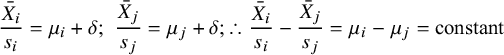 $$\begin{align*}\frac{\bar{X}_i}{s_i} = {\mu}_i+\delta; \kern0.36em \frac{\bar{X}_j}{s_j} = {\mu}_j+\delta; \therefore \frac{\bar{X}_i}{s_i}-\frac{\bar{X}_j}{s_j} = {\mu}_i-{\mu}_j = \mathrm{constant}\end{align*}$$
This assumes that the standardising constants are constant between trials, contrary to the facts of range variation. The Scale-SMD hypothesis is exactly the same, except that range variation is eliminated by fixing the standardising constants for each scale.
The RoM hypothesis is that the ratio of the mean outcomes is constant, independent of treatment.
 $$\begin{align*}\mathit{\log}\left(\bar{X}_i\right) = {\mu}_i+\delta; \kern0.36em \log \left(\bar{X}_j\right) = {\mu}_j+\delta; \therefore \frac{\bar{X}_i}{\bar{X}_j} = \mathit{\exp}\left({\mu}_i-{\mu}_j\right) = \mathrm{constant}.\end{align*}$$
In this paper, we compare the performance of different standardisation and ratio methods in a network meta-analysis of 14 treatments for depression, reported on five different scales. We compare Study-SMD and Scale-SMD, with and without meta-regression (MR) against baseline SD, and RoM. Our objective is to develop methods for deciding which of these models provides the best fit to the data, the most precise estimates, and the lowest between-study heterogeneity. We illustrate these methods by applying them to a frequently used form of PCRO data. We also investigate the impact of model choice on treatment recommendations.
2 Methods
2.1 Dataset: Pharmacological treatments for depression
We use a dataset of 161 studies which were a subset of studies from NICE guideline NG222 that compared pharmacological treatments for more severe (moderate and severe) depression in adults from a larger review. 19 Studies were included only if they reported findings on the Hamilton Depression Rating Scale (HAMD-17, HAMD-21, HAMD-24), the Beck Depression Inventory (BDI), or the Montgomery-Asberg Depression Scale (MADRS). There were comparisons between 14 active treatments, pill placebo, and “no treatment”. Two studies that reported exceptionally low standard deviations (0.46 and 0.65 on the HAMD-21 scale) were excluded. The evidence network was highly connected with multiple trials of each active treatment (Figure 1). There was direct evidence on 59 of the possible 120 pair-wise comparisons, and they were informed by between 1 and 14 trials (median 2 trials). Because we wished to compare models with and without meta-regression, only studies reporting baseline severity for the whole sample were included.
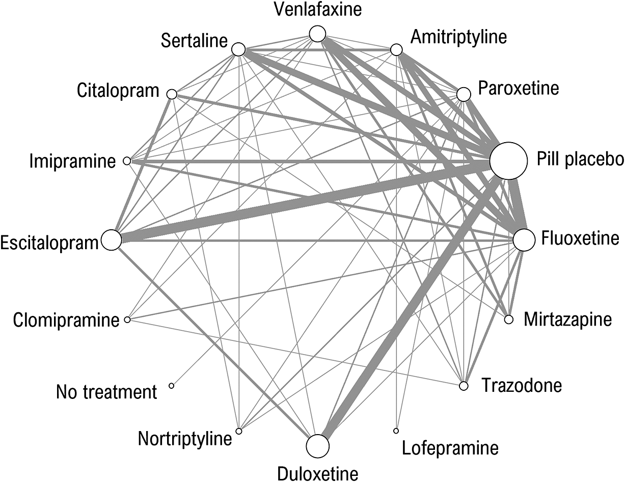
Figure 1 Network of evidence on 14 pharmacological treatments of more severe depression, no treatment and pill placebo. The thickness of edges is proportional to the number of studies and the size of nodes is proportional to the number of participants receiving the treatment.
Data were extracted for NG222 in one of three different formats in the following priority order:
-
i) mean change-from-baseline (CFB) with standard error for each study arm
-
ii) mean depression scores at baseline and follow-up with standard errors for each study arm
-
iii) mean depression score at follow-up, with standard error for each study arm
following guidance in Guideline Methodology Document 2Reference Daly, Welton, Dias, Anwer and Ades 18 for data extraction to fit SMD models.
Network diagrams of trials with data in these three formats, along with the types of data (by format and scale) extracted for each treatment, are shown in the Supplementary Materials (Supplementary Figure S1 and Supplementary Table S1, respectively). However, when fitting a RoM model, the recommendedReference Daly, Welton, Dias, Anwer and Ades 18 priority order of data extraction would instead be formats (ii), (iii), then (i), since an assumption of additivity is inherent in calculating CFB, and therefore it is least preferred when fitting a multiplicative model. We, therefore, ran a sensitivity analysis using this alternative prioritisation of data formats; however, this was constrained by available data in the NG222 dataset, as we did not re-extract data from these studies.
For studies reporting baseline and follow-up measures, we need to assume a value for the correlation,
 ${\rho}_i$
, between baseline and follow-up outcomes to form the standard error of the CFB, and also to estimate RoM from studies that only report in CFB data format (see Supplementary Materials, Appendix 1). The correlation was assumed to be 0.3, which was the median correlation in the studies where it could be estimated in the NG222.
19
As a sensitivity analysis, we also examined results with the correlation set to 0.5.
${\rho}_i$
, between baseline and follow-up outcomes to form the standard error of the CFB, and also to estimate RoM from studies that only report in CFB data format (see Supplementary Materials, Appendix 1). The correlation was assumed to be 0.3, which was the median correlation in the studies where it could be estimated in the NG222.
19
As a sensitivity analysis, we also examined results with the correlation set to 0.5.
2.2 Descriptive analyses
Two descriptive analyses were run, to test or to assess the assumptions of the different models. Bartlett’s test of equality of variances was applied to assess the assumption of equality of SDs in different studies reported on the same scale.Reference Snedecor and Cochrane 20 The relation between mean scores at baseline (or follow-up) and the SD of scores at baseline (or follow-up) is an indicator of heteroscedasticity.
2.3 Standardised Mean Difference (SMD) measures
The standardised mean difference divides the mean difference between treatment arms by a standardising constant
 $s$
.
$s$
.
For our depression model, the mean difference represents the difference between treatments in the mean CFB. Let
 $mea{n}_{B,k}$
be the mean outcome at baseline and
$mea{n}_{B,k}$
be the mean outcome at baseline and
 $mea{n}_{F,k}$
the mean outcome at follow-up for treatment
$mea{n}_{F,k}$
the mean outcome at follow-up for treatment
 $k$
, then the SMD for the mean CFB is:
$k$
, then the SMD for the mean CFB is:
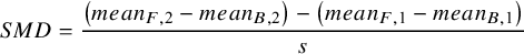 $$\begin{align}SMD = \frac{\left( mea{n}_{F,2}- mea{n}_{B,2}\right)-\left( mea{n}_{F,1}- mea{n}_{B,1}\right)}{s}\end{align}$$
We prioritise modelling the CFB when possible, as it accounts for baseline differences, but we can use follow-up means if no other data are available.
We explore two alternative standardising constants
 $s$
, one using the study-specific SD and the other using a scale-specific SD, and refer to the resulting SMD as Study-SMD and Scale-SMD respectively.
$s$
, one using the study-specific SD and the other using a scale-specific SD, and refer to the resulting SMD as Study-SMD and Scale-SMD respectively.
2.3.1 Study-specific SMD
The most common approach is to standardise by the pooled baseline SD specific to the study, termed Cohen’s d.
Reference Cohen
21
In this case, the SDs at baseline from each arm,
 $k$
, are combined to give a single pooled SD for the study
$k$
, are combined to give a single pooled SD for the study
 $i$
:
$i$
:
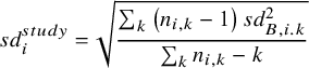 $$\begin{align}s{d}_i^{study} = \sqrt{\frac{\sum_k\left({n}_{i,k}-1\right)s{d}_{B,i.k}^2}{\sum_k{n}_{i,k}-k}}\end{align}$$
where
 ${n}_{i,k}$
is the number of patients randomised, and
${n}_{i,k}$
is the number of patients randomised, and
 $s{d}_{B,i,k}$
is the baseline SD for study
$s{d}_{B,i,k}$
is the baseline SD for study
 $i$
arm
$i$
arm
 $k$
. We use the baseline SD to compute the standardising constant because it is not influenced by treatment, so better reflects the SD of the outcome scale in the population recruited to the study and can be estimated from all trial arms. Note, that we do not consider the situation where interest is in the treatment effect on standard deviation of outcomes.
$k$
. We use the baseline SD to compute the standardising constant because it is not influenced by treatment, so better reflects the SD of the outcome scale in the population recruited to the study and can be estimated from all trial arms. Note, that we do not consider the situation where interest is in the treatment effect on standard deviation of outcomes.
2.3.2 Scale-specific SMD
Ideally, a scale-specific standardisation constant would be obtained from a large representative population where all scales have been measured. However, in the absence of such a study, we can pool the study-specific baseline SDs,
 $s{d}_i^{study}$
, across all those studies that report on a specific scale
$s{d}_i^{study}$
, across all those studies that report on a specific scale
 $j$
:
$j$
:
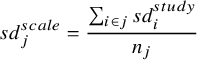 $$\begin{align}s{d}_j^{scale} = \frac{\sum_{i\in j}s{d}_i^{study}}{n_j}\end{align}$$
where
 $i\in j$
indicates studies reporting scale
$i\in j$
indicates studies reporting scale
 $j$
, and
$j$
, and
 ${n}_j$
the number of studies that report scale
${n}_j$
the number of studies that report scale
 $j$
.
$j$
.
 $s{d}_j^{scale}$
is used as the standardising constant for those studies reporting scale
$s{d}_j^{scale}$
is used as the standardising constant for those studies reporting scale
 $j$
.
$j$
.
2.4 Ratio of Means (RoM) measure
If both baseline and follow-up measures are available then a multiplicative effect measure for the ratio change from baseline is the Ratio of Ratio of Means (RoRoM), calculated as:
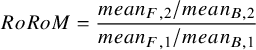 $$\begin{align}RoRoM = \frac{mean_{F,2}/mean_{B,2}}{mean_{F,1}/mean_{B,1}}\end{align}$$
If only follow-up measures are available, then the Ratio of Means (RoM) is:
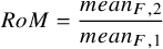 $$\begin{align}RoM = \frac{mean_{F,2}}{mean_{F,1}}\end{align}$$
Similarly to CFB, RoRoM adjusts for baseline imbalances, and so is preferred over RoM when it can be calculated. However, both RoRoM and RoM can be pooled to obtain an estimate of the treatment effect.
The RoM is not easily interpretable when outcome scores can have both positive and negative signs. However, if baseline values are available, they can be combined with the CFB to obtain baseline and follow-up means so that the RoRoM in equation (4) can be calculated (see Appendix 1).Reference Daly, Welton, Dias, Anwer and Ades 18
2.5 Network Meta-Analysis (NMA) model
Network meta-analysis (NMA) enables evidence to be pooled on multiple treatments where the evidence forms a connected network (Figure 1). We used a Bayesian NMA model,Reference Lu and Ades
22
,
Reference Dias, Sutton, Ades and Welton
23
where we adapted the likelihood and link functions to pool the various data formats to inform the SMD and RoM models (see Supplementary Materials, Appendix 1). The NMA model is put on the parameter
 ${\theta}_{i,k}$
for arm
${\theta}_{i,k}$
for arm
 $k$
of study
$k$
of study
 $i$
which represents the standardised mean for the SMD models, and represents the log-mean outcome for the ROM model. The NMA model is the same for the SMD and RoM models, but the parameters have different interpretations:
$i$
which represents the standardised mean for the SMD models, and represents the log-mean outcome for the ROM model. The NMA model is the same for the SMD and RoM models, but the parameters have different interpretations:
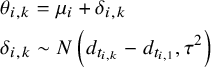 $$\begin{align}&{\theta}_{i,k} = {\mu}_i+{\delta}_{i,k}\nonumber\\&{\delta}_{i,k}\sim N\left({d}_{t_{i,k}}-{d}_{t_{i,1}},{\tau}^2\right)\end{align}$$
where
 ${\mu}_i$
is the standardised mean (or log-mean) for the treatment on arm 1 of study
${\mu}_i$
is the standardised mean (or log-mean) for the treatment on arm 1 of study
 $i$
, and
$i$
, and
 ${\delta}_{i,k}$
is the study-specific SMD (or log RoM) for arm
${\delta}_{i,k}$
is the study-specific SMD (or log RoM) for arm
 $k$
relative to arm 1 of study
$k$
relative to arm 1 of study
 $i$
. For a random effects NMA it is assumed that the study-specific SMDs (or log RoMs) come from a Normal distribution, where
$i$
. For a random effects NMA it is assumed that the study-specific SMDs (or log RoMs) come from a Normal distribution, where
 ${t}_{i,k}$
indicates the treatment on arm
${t}_{i,k}$
indicates the treatment on arm
 $k$
of study
$k$
of study
 $i$
,
$i$
,
 ${d}_k$
represents the SMD (or log RoM) for treatment
${d}_k$
represents the SMD (or log RoM) for treatment
 $k$
relative to treatment 1 (the reference treatment for the network), and
$k$
relative to treatment 1 (the reference treatment for the network), and
 $\tau$
represents the between-study standard deviation on the linear predictor scale. Based on previous analyses of treatments for depression it is expected that there will be a degree of heterogeneity, and so we did not fit fixed effect models.
$\tau$
represents the between-study standard deviation on the linear predictor scale. Based on previous analyses of treatments for depression it is expected that there will be a degree of heterogeneity, and so we did not fit fixed effect models.
Estimates of the pooled RoM for treatment
 $k$
relative to treatment 1 is obtained by exponentiating the log RoM:
$k$
relative to treatment 1 is obtained by exponentiating the log RoM:
 $$\begin{align}Ro{M}_k = {e}^{d_k}\end{align}$$
By using the exact same dataset and likelihood for all the models, we are able to combine multiple data types (follow-up scores and CFB) and to provide valid comparisons of goodness of fit statistics for all five models.
2.6 Meta-regression of SMD on baseline severity
Versions of both Scale- and Study-SMD models were created in which a regression term for baseline severity was introduced in all active vs inactive comparisons, which we term Scale-SMD-MR and Study-SMD-MR respectively (see Appendix 1 for details).
2.7 Model comparison and selection
The models we compared were: SMD standardised with study-specific SD (Study-SMD); SMD standardised with scale-specific SD (Scale-SMD); Study-SMD with meta-regression for severity (Study-SMD-MR); Scale-SMD with meta-regression for severity (Scale-SMD-MR); and RoM. Models were compared using the posterior mean residual deviance,
 $\bar{D}$
, as a measure of model fit, and the Deviance Information Criterion (DIC), which penalises the deviance by a measure of model complexity, the number of effective parameters,
$\bar{D}$
, as a measure of model fit, and the Deviance Information Criterion (DIC), which penalises the deviance by a measure of model complexity, the number of effective parameters,
 $pD$
.Reference Spiegelhalter, Best, Carlin and van der Linde
24
$pD$
.Reference Spiegelhalter, Best, Carlin and van der Linde
24
 $pD$
is calculated as the sum over study arms of the difference between the posterior mean deviance and the deviance evaluated at the posterior mean of the mean value of
$pD$
is calculated as the sum over study arms of the difference between the posterior mean deviance and the deviance evaluated at the posterior mean of the mean value of
 ${\theta}_{ik}$
. Models with lower
${\theta}_{ik}$
. Models with lower
 $\bar{D}$
and DIC are preferred.
$\bar{D}$
and DIC are preferred.
We report the posterior median and 95% credible intervals for the between-study standard deviation, as a measure of heterogeneity. However, it is important to note that these are not comparable across different outcome scales. To overcome this, we introduce a scale-independent measure of heterogeneity, percentage shrinkage, that can be calculated using
 $pD$
.
$pD$
.
For a fixed effect model, all study estimates are equal for the same comparison, so there is no heterogeneity (
 $\tau = 0$
), 100% shrinkage and the effective number of model parameters is
$\tau = 0$
), 100% shrinkage and the effective number of model parameters is
 ${p}_D = ns+ nt-1$
, for the
${p}_D = ns+ nt-1$
, for the
 $ns$
study baseline parameters, and
$ns$
study baseline parameters, and
 $nt-1$
treatment effects relative to reference treatment 1. At the other extreme, for an “independent effects” model where each study effect is independent of all other study effects, there is a high value of
$nt-1$
treatment effects relative to reference treatment 1. At the other extreme, for an “independent effects” model where each study effect is independent of all other study effects, there is a high value of
 $\tau$
, which will depend on the scale of analysis, 0% shrinkage, and the effective number of model parameters is
$\tau$
, which will depend on the scale of analysis, 0% shrinkage, and the effective number of model parameters is
 ${p}_D = na$
, for the number of study arms
${p}_D = na$
, for the number of study arms
 $na$
, reflecting a different parameter for each study arm, which is an upper bound for
$na$
, reflecting a different parameter for each study arm, which is an upper bound for
 ${p}_D$
. Random effects models with a value of
${p}_D$
. Random effects models with a value of
 ${p}_D$
lying between these extremes exhibit a degree of heterogeneity, with values closer to the upper bound indicating higher levels of heterogeneity. We measure this using the % shrinkage defined as:
${p}_D$
lying between these extremes exhibit a degree of heterogeneity, with values closer to the upper bound indicating higher levels of heterogeneity. We measure this using the % shrinkage defined as:
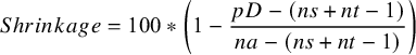 $$\begin{align}Shrinkage = 100\ast \left(1-\frac{pD-\left( ns+ nt-1\right)}{na-\left( ns+ nt-1\right)}\right)\end{align}$$
with low heterogeneity having a % shrinkage closer to 100%, and those with higher heterogeneity having a % shrinkage closer to 0%.
Where baseline and CFB or baseline and follow-up values are used in a bivariate likelihood, there are two data points per study arm, so
 $na$
is replaced with
$na$
is replaced with
 $\left(n{a}^{univ}+2n{a}^{biv}\right)$
in (9), where
$\left(n{a}^{univ}+2n{a}^{biv}\right)$
in (9), where
 $n{a}^{univ}$
is the number of univariate study arms and
$n{a}^{univ}$
is the number of univariate study arms and
 $n{a}^{biv}$
is the number of bivariate study arms.
$n{a}^{biv}$
is the number of bivariate study arms.
In the depression example,
 $ns = 161, nt = 16$
, and
$ns = 161, nt = 16$
, and
 $na = 340$
, with 271 study arms reported as CFB or baseline and follow-up,
$na = 340$
, with 271 study arms reported as CFB or baseline and follow-up,
 $n{a}^{biv}$
, and 69 study arms reported as final values,
$n{a}^{biv}$
, and 69 study arms reported as final values,
 $n{a}^{uni}$
, so
$n{a}^{uni}$
, so
 ${p}_D$
lies between 176 and 611.
${p}_D$
lies between 176 and 611.
2.8 Transformation of SMDs and RoM to a common measurement scale (HAMD-17)
To compare treatment effects from SMD and RoM models, the relative treatment effects
 ${d}_k$
were transformed to a mean difference on the most frequently reported scale: HAMD-17. This required an assumption about the mean and SD on the reference treatment 1 on the HAMD-17 scale. Treatment effects estimated from SMD models,
${d}_k$
were transformed to a mean difference on the most frequently reported scale: HAMD-17. This required an assumption about the mean and SD on the reference treatment 1 on the HAMD-17 scale. Treatment effects estimated from SMD models,
 ${d}_k^{SMD}$
, were back-transformed using the mean pooled baseline SD for the HAMD-17 scale,
${d}_k^{SMD}$
, were back-transformed using the mean pooled baseline SD for the HAMD-17 scale,
 $s{d}_B^{HAMD-17}$
:
$s{d}_B^{HAMD-17}$
:
 $$\begin{align}{d}_k^{HAMD-17} = {d}_k^{SMD}\ast s{d}_B^{HAMD-17}\end{align}$$
Similarly, between-study SD for the SMD models was back-transformed onto the HAMD-17 scale using the mean pooled baseline SD for the HAMD-17 scale,
 $s{d}_B^{HAMD-17}$
.
$s{d}_B^{HAMD-17}$
.
Treatment effects estimated from the RoM model were back-transformed to a mean difference on the HAMD-17 using a representative mean HAMD-17 score on the reference treatment,
 ${\bar{\mu}}_{HAMD-17}$
:
${\bar{\mu}}_{HAMD-17}$
:
 $$\begin{align}{d}_k^{HAMD-17} = \left({\bar{\mu}}_{HAMD-17}\ast {e}^{d_k}\right)-{\bar{\mu}}_{HAMD-17}\end{align}$$
where
 ${\bar{\mu}}_{HAMD-17}$
was the CFB calculated from the mean at follow-up values (−6.4 and 15.7 respectively) taken from the largest study reporting depression scores for pill placebo (the reference treatment) on the HAMD-17 scale.Reference Tollefson and Holman
25
,
Reference Tollefson, Bosomworth, Heiligenstein, Potvin and Holman
26
${\bar{\mu}}_{HAMD-17}$
was the CFB calculated from the mean at follow-up values (−6.4 and 15.7 respectively) taken from the largest study reporting depression scores for pill placebo (the reference treatment) on the HAMD-17 scale.Reference Tollefson and Holman
25
,
Reference Tollefson, Bosomworth, Heiligenstein, Potvin and Holman
26
2.9 Treatment recommendations
We also compare the impact of the different models on resulting treatment recommendations based on five different decision rules:
-
i) the treatment with the highest posterior mean estimate of efficacy.
-
ii) all treatments where the 95% credible interval (CrI) of the treatment effect relative to pill placebo did not include zero.
-
iii) all treatments where the 95% CrI of the treatment effect relative to pill placebo was greater than a clinically important difference of 1 unit on the HAMD-17 scale, which is approximately 0.25 SD units (Table 1).
-
iv) As (iii) above, but limited to treatments that were not inferior to the best treatment (ie the 95%CrI for the difference did not include zero).
-
v) The set of treatments that satisfy decision rule (iii) and which were not inferior to any other treatment (ie the 95% credible interval on the difference does not include 0). This rule is a version of a proposal from the GRADE Working Party, with the threshold value set to zero.Reference Brignardello-Petersen, Florez and Izcovich 27
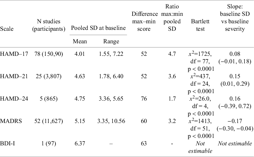
Table 1 Variation in baseline SD within each scale and regression of baseline SD against baseline severity
2.10 Software, model estimation, and priors
Models were estimated by Bayesian Markov chain Monte Carlo in WinBUGS 1.4.3.Reference Spiegelhalter, Thomas, Best and Lunn 28 Models were run with three chains with the first 40,000 iterations discarded as burn-in. Chain convergence was assessed with Brooks-Gelman-Rubin plots and chain mixing with trace and history plots. Following burn-in and convergence, 80,000 iterations from each of the three chains were used for inference.
Vague priors were provided for estimates of treatment effect,
 ${d}_k$
, study-level baselines,
${d}_k$
, study-level baselines,
 ${\mu}_i$
, and between-study SD,
${\mu}_i$
, and between-study SD,
 $\tau$
.
$\tau$
.
 $$\begin{align*}{d}_k\sim N\left(0,10{0}^2\right)\end{align*}$$
 $$\begin{align*}{\mu}_i\sim N\left(0,10{0}^2\right)\end{align*}$$
 $$\begin{align}\tau \sim U\left(0,5\right)\end{align}$$
Data visualisation was performed in R version 4.3.1Reference Brignardello-Petersen, Florez and Izcovich 27 using packages ggplot2, ggpubr, and viridis.
3 Results
3.1 Descriptive analysis
Bartlett testsReference Snedecor and Cochrane 20 of the null hypothesis of equal variance in studies reporting on the same scale indicated statistically large differences between the baseline standard deviations (SDs) from each study. The ratio of maximum to minimum baseline SDs varied from 1.7 (HAMD-24) to 4.7 (HAMD-17) (Table 1), with a weighted average of 4.0.
For the three HAMD scales, mean depression scores at baseline increased with baseline SD, but this was not observed with the MADRS scale (Table 1, Figure 2).
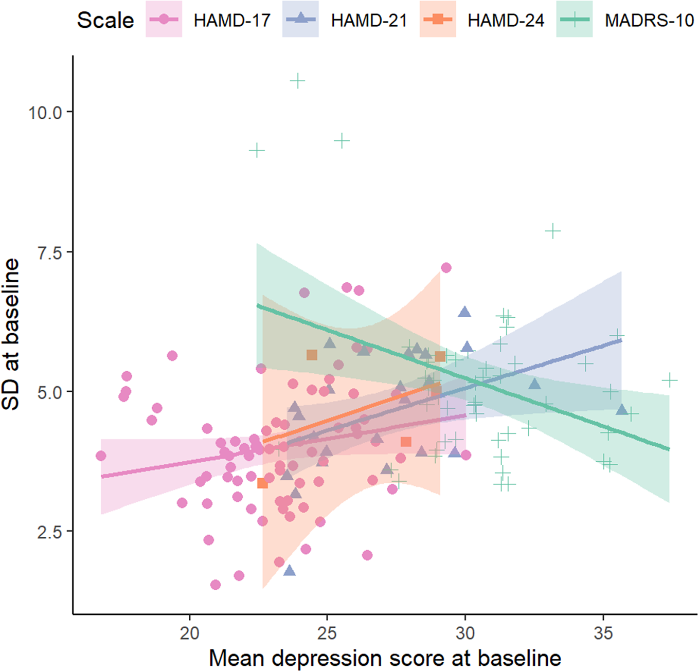
Figure 2 The relationship between the baseline pooled standard deviation and mean depression score at baseline. Results are shown by scale for HAMD-17, HAMD-21, HAMD-24 and MADRS scales. BDI-I could not be plotted because it was reported in a single study.
Table 2 Model fit statistics and heterogeneity estimated within each of the five models
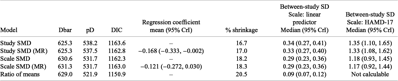
Note: Fit statistics: posterior mean residual deviance (relative to 611 data points), DIC, and percentage shrinkage. Coefficient of meta-regression (MR) on baseline severity. The posterior median of between-study SD with the 95% credible interval (CrI) on both the linear predictor scale and, for SMD models, on the HAMD-17 scale.
3.2 Model fit, heterogeneity, relative effects, and their precision
Study-SMD and Study-SMD-MR models have a slightly lower posterior mean residual deviance (Table 2), indicating a better fit compared to the other measures. The closer fit is the result of greater model complexity, reflected in the higher
 $pD$
, and larger heterogeneity in treatment effects, as seen in the between-study SD. RoM has the best fit given model complexity with the lowest DIC. Scale-SMD and Scale-SMD-MR models have a similar fit to RoM, but higher DIC reflecting the higher effective number of parameters. These results on DIC reflect the greater shrinkage (reduced heterogeneity) seen with RoM (20.5%), with an intermediate degree of shrinkage with the Scale-SMD (18.2%), and lower shrinkage (higher heterogeneity) with Study-SMD (16.7%). The degree of heterogeneity, as measured by the between-study SD, was 13% lower in the Scale-SMD than in the Study-SMD models (Table 2).
$pD$
, and larger heterogeneity in treatment effects, as seen in the between-study SD. RoM has the best fit given model complexity with the lowest DIC. Scale-SMD and Scale-SMD-MR models have a similar fit to RoM, but higher DIC reflecting the higher effective number of parameters. These results on DIC reflect the greater shrinkage (reduced heterogeneity) seen with RoM (20.5%), with an intermediate degree of shrinkage with the Scale-SMD (18.2%), and lower shrinkage (higher heterogeneity) with Study-SMD (16.7%). The degree of heterogeneity, as measured by the between-study SD, was 13% lower in the Scale-SMD than in the Study-SMD models (Table 2).
The regression coefficients in the meta-regression models were negative (Table 2), indicating a stronger treatment effect in trials whose study populations were more severely depressed at the outset. This effect was somewhat stronger with the Study-SMD outcome measure. The global fit and shrinkage statistics of the SMD meta-regression models were no different from their non-regression counterparts.
The effects of all treatments relative to pill placebo on the HAMD-17 scale appear in Table 3 and in Figure 3 in the form of a forest plot as median estimates with credible and predictive intervals. Predictive intervals depict where the treatment effect from a new study might lie and are generated from the between-study SD, therefore they reflect the heterogeneity within the modelled data. The predictive intervals were narrower in the Scale-SMD models than in the Study-SMD models.
Effects of active treatments relative to the best treatment on each scale appear in Supplementary Table S2.
3.3 Treatment recommendations
The treatment recommendations generated by the different models are presented in Table 4, using five different decision rules. The single best treatment (highest expected efficacy) was Amitriptyline for the RoM model and Scale-SMD models, and Mirtazapine for the Study-SMD models. The second decision rule selected all treatments with evidence of effect “significantly” better than pill placebo (that is where the 95%CrI did not cross zero). All active treatments qualified on all models.
Table 3 The mean difference of treatments relative to pill placebo, presented as units on the HAMD-17 scale, with their 95% CrI
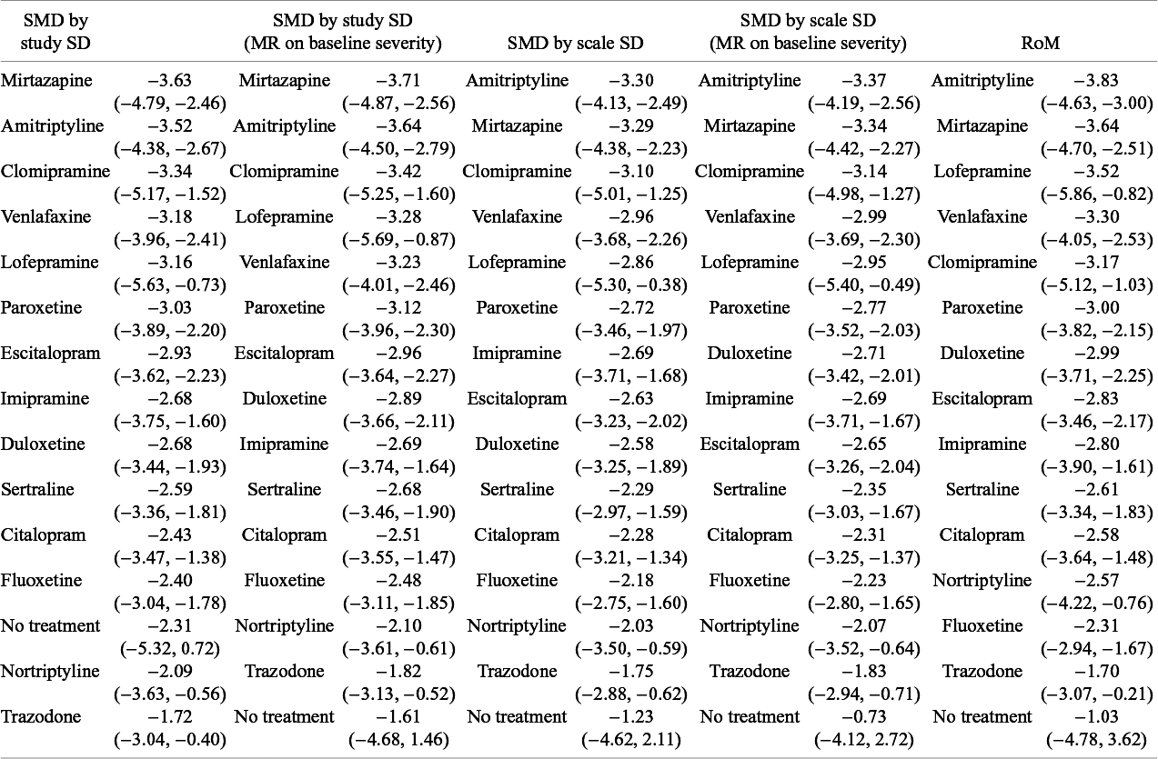
Note: Estimates are presented from models of depression score standardised as SMDs by study-level and scale-level pooled SD, with and without meta-regression (MR) on baseline severity, and a model of the ratio of means (RoM).
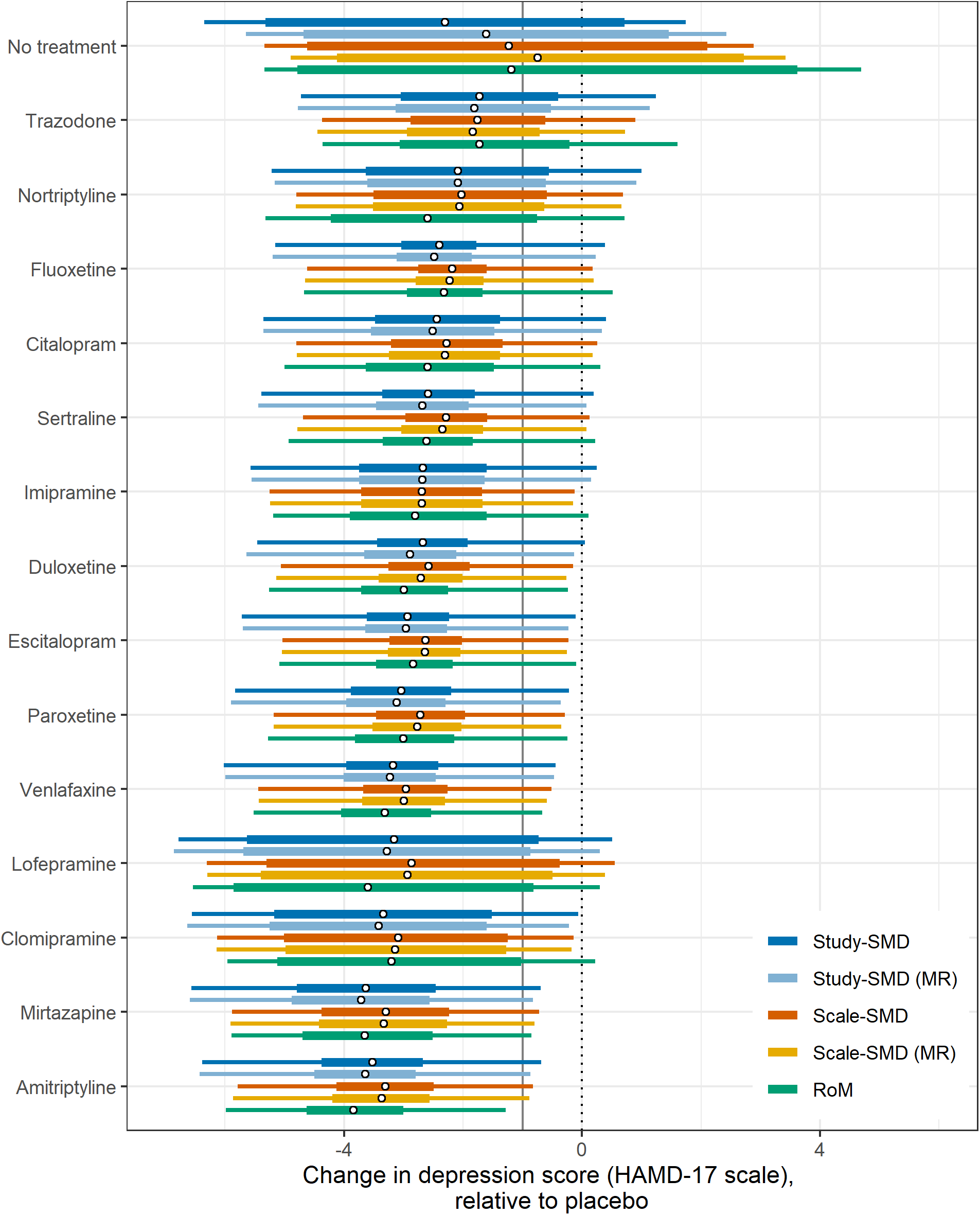
Figure 3 Treatment effect vs placebo as change in depression score on the HAMD-17 scale by model. In each case, circular points indicate the median estimate, thick bars indicate the 95% credible interval (CrI) and thin bars indicate the 95% prediction interval, for each treatment vs placebo. Treatments are ordered by median treatment effect under the RoM model. The vertical grey line indicates one unit on the HAMD-17 scale.
If decision-makers were to recommend all treatments that were better than placebo by at least 1 HAMD-17 unit, the third decision rule, all five models pick out the same 11 treatments, and exclude trazodone, nortriptyline, and lofepramine.
The fourth approach selects from the above 11 treatments all those that are also not inferior to the best treatment. In this case, RoM picks out only seven treatments besides the best, Scale-SMD models a further eight, and Study-SMD models a further nine. Our fifth decision rule, based on GRADE recommendations, identifies a set of treatments that is inferior to no other treatment, again using a 95% credible limit. In this case, all five models picked out the same three treatments. Unlike the first three decision rules, which are driven by differences between active treatments and placebo, the fourth and fifth depend on differences between the active treatments. It seems that discrimination between active treatments is better in RoM models than in Scale-SMD, and that Scale-SMD models discriminate better than Study-SMD.
3.4 Sensitivity analyses
The results from the sensitivity analysis using a different prioritisation of data format are given in Supplementary Materials, Appendix 3. The findings were generally similar (Supplementary Materials, Appendix 3, Supplementary Table S3) to those from the main analysis (Table 2), although the benefits of the RoM model compared to the Scale-SMD models were minimal. All five models selected the same treatment as in the main analysis, and the results with the different decision rules differed only slightly from the main analysis (Supplementary Materials Appendix 3). Better discrimination between active treatments on the HAMD-17 scale was observed for the RoM model in both analyses.
A sensitivity analysis setting the before-after correlation at 0.5, as opposed to our base-case 0.3, had negligible effects on shrinkage. Shrinkage was lowered from 17% to 16% for Study-SMD, from 18% to 17% for Scale-SMD, and remained at 21% for RoM.
Table 4 Treatment recommendations based on each model, ranked by efficacy, according to five decision rules
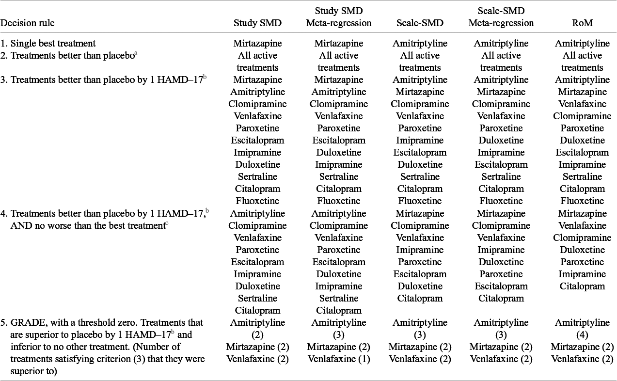
a X better than Y means that the 95%CrI on the (X–Y) difference did not include zero.
b X better than Y by more than 1 HAMD-17 unit means that the 95% CrI on the (X–Y) difference did not include −1.0.
c X no worse than Y means that the 95%CrI on the (X-Y) difference did not include zero.
4 Discussion
4.1 Summary of findings
In this dataset, which was typical of pharmaceutical trials for more severe depression, the RoM model performed better than any SMD model. This assessment was based on lower DIC and greater shrinkage of estimates. Furthermore, examination of differences between active treatments’ effects on the HAMD-17 scale produced evidence that treatment effects were estimated with greater precision in the RoM models than in the Scale-SMD model. The Scale-SMD model gave a similar fit to RoM but had higher heterogeneity.
Scale-SMD models performed better than Study-SMD, giving lower heterogeneity and more precise estimates, by about 6%. A core assumption of the Study-SMD method is that all the studies that report on the same scale should have the same SD.Reference Higgins, Li, Deeks, Higgins and Thomas 15 Hunter and SchmidtReference Hunter and Schmidt 17 regarded the changes in SMDs due to different study variances as “range variation” artefacts that required removing, and they advocated a form of Scale-SMD approach. In our dataset, range variation, which is generated by sampling variation as well as between-study population differences, was statistically and materially highly significant, with study SDs reported on the same scale varying over an average 4.0-fold range. The effect of the Study-SD method is therefore to multiply relative treatment effects by an arbitrary number between 1 and 4. Similar findings have been reported in trials reporting on the Liebowitz Social Anxiety Scale.Reference Ades, Lu, Dias, Mayo-Wilson and Kounali 29
Scale-SMD models represent an improvement on Study-SMDs because they avoid range variation by using a single normalising SD for each scale. To create a reference SD we used the average SD over the available studies using that scale. This is an imperfect solution, as it risks introducing random error when there are small numbers of studies. The ideal would be to use reference SDs from a single large population study. However, large population studies looking at the full range of scales are uncommon. Alternatively, it may be possible to derive reference SDs by modelling large collections of trials or observational studies.
4.2 Criteria employed in this study, and robustness of findings
The criteria used here to compare models were: global model fit; percentage shrinkage (a scale-independent measure of heterogeneity); DIC, which is model fit penalised for complexity; and precision of relative effects. These are in line with previous literature on the choice of scale in meta-analysis, which has focused on between-study heterogeneity measured by the Q-statistic,Reference Friedrich, Adhikari and Beyenegh 9 , Reference Deeks 30 , Reference Engels, Schmid, Terrin, Olkin and Lau 31 or on both Q-statistics and precision of estimates.Reference Friedrich, Adhikari and Beyene 32 , Reference Takeshima, Sozu, Tajika, Ogawa, Hayasaka and Furukawa 33 Another measure that has been used is the percentage of study effects within the 95% confidence interval of the pooled effect.Reference Takeshima, Sozu, Tajika, Ogawa, Hayasaka and Furukawa 33 A study comparing five different effect measures in an NMA of trials reporting binary data used global fit statistics and DIC.Reference Caldwell, Welton, Dias and Ades 34
A limitation of reliance on aggregated data is that assumptions have to be made about correlations between baseline and follow-up scores. Our results assumed a correlation of 0.3, based on the evidence available; a sensitivity analysis with a correlation of 0.5 showed a greater advantage of RoM models. A second sensitivity analysis examined the priority order for data extraction. The base-case analysis prioritised (i) CFB, (ii) baseline and follow-up, and (iii) follow-up only. Results with an alternative ordering (ii, iii, and i) produced similar findings although there was no longer any difference between Scale-SMD and RoM methods. However, the better discrimination between treatments observed in the base-case analysis was also evident in this sensitivity analysis. It should be noted that this analysis was limited by the available data (which had been extracted following the priorities for SMDs).
4.3 Generality of findings
A limitation of the study is that it is restricted to a single dataset of trials, which includes only pharmaceutical interventions, for a particular severity range—more severe—of a specific disorder, depression. It is therefore unclear how far one can generalise from the present results to other PCROs consisting of correlated sums of sub-scale scores, let alone to other types of continuous outcomes. Although studies comparing RoM with Study-SMD in large collections of pair-wise meta-analyses have reported more heterogeneity in SMD models,Reference Friedrich, Adhikari and Beyenegh 9 this finding may be due to the poor performance of Study-SMD, and the comparison may yield different results if Scale-SMD were used instead. We would in any case urge caution before adopting any “one-size-fits-all” solution, and recommend that further studies are conducted, along the lines of the present study, using large networks of trials to examine commonly used PCROs. Separate investigations are required in each clinical area of psychiatric, neurologic, and other fields where PCROs are used.
4.4 Minimally important difference
Another approach, attracting increasing attention, is to standardise by dividing mean treatment effects in each trial by the MID, generating treatment effects in MID units. Some researchers regard MIDs as more easily interpretable than either SMDs or the units of the original scales.Reference Thorlund, Walter, Johnston, Furukawa and Guyatt 1 , Reference Johnston, Thorlund and Schunemann 3 , Reference Jaeschke, Singer and Guyatt 16 Interestingly, in parallel to SMDs, both scale-specificReference Thorlund, Walter, Johnston, Furukawa and Guyatt 1 , Reference Jaeschke, Singer and Guyatt 16 , Reference Schunemann, Vist, Higgins, Higgins and Thomas 35 and study-specificReference Johnston, Thorlund, Da Costa, Furukawa and Guyatt 36 MIDs have been proposed, the latter for studies using scales for which no MID estimate is available. MIDs have also been expressed as percent improvement, indicating a proportional rather than additive effect, most notably in studies of depression.Reference Button, Kounali and Thomas 37 , Reference Bauer-Staeb, Kounali and Welton 38 The adoption of a MID approach does not in itself, therefore, contribute directly to the issues addressed in this paper: whether treatment effects are additive or multiplicative, and the choice of scale-specific or study-specific standardisation. Researchers using MID face several additional challenges: multiple ways of constructing and/or presenting the MID,Reference Copay, Subach, Glassman, Polly and Schuler 39 , Reference Johnston, Patrick and Thorlund 40 the extreme variability of estimates,Reference Chung, Copay, Olmscheid, Campbell, Walker and Chutkan 41 – Reference Kolin, Moverman and Pagani 43 and between-patient variation.Reference Bauer-Staeb, Kounali and Welton 38 , Reference Shrier, Christensen, Juhlc and Beyene 44 Before choosing a solution to the problems posed by outcomes reported on multiple scales, we believe the first priority must be to determine whether treatment effects are multiplicative or additive.
4.5 Impact of choice of scale on treatment recommendations
Although there were differences between the five models in treatment rankings, including differences regarding which treatment was best, there was a high level of concordance. A decision rule similar to the one proposed by the GRADE Working GroupReference Brignardello-Petersen, Florez and Izcovich 27 picked out the same three treatments under all five models. The relative insensitivity of treatment rankings to the choice of scale has been observed in previous NMAs of binomial data.Reference Caldwell, Welton, Dias and Ades 34 One should not conclude from this that the choice of scale does not matter, as it can have a substantial impact on the estimates themselves and their precision.Reference Caldwell, Welton, Dias and Ades 34 The formulation of decision rules for recommending treatments following an NMA is a topic calling for further research, particularly decision rules that take uncertainty into account.Reference Ades, Pedder and Davies 45 Rules such as those proposed by GRADE,Reference Brignardello-Petersen, Florez and Izcovich 27 because they can recommend treatments that are not “significantly” different from the best treatment, may have the unwanted effect of privileging treatments with more uncertain evidence.
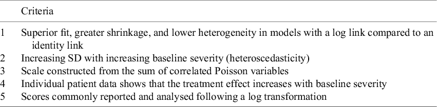
4.6 Recommendations regarding the choice of scale
A decision about whether treatment effects are multiplicative or additive should be based on all the evidence available, including clinical opinion.Reference Deeks 30 Table 5 summarises the kinds of evidence that would support the conclusion that effects are multiplicative. Depression scales score on the first four of the five criteria. Thus, although the empirical evidence on model fit and shrinkage in this paper is not strong, in combination with other evidence, we would regard the overall evidence for multiplicative effects as strong enough to favour RoM as the default.
Table 5 Criteria supporting the assumption of multiplicative treatment effects
For measurement scales where additivity can be assumed, we would recommend scale-specific standardisation by SMD or, if reliable estimates exist, MID. This is supported by the results reported here and is based on well-established arguments in textbooks and tutorial papers.Reference Guyatt, Thorlund and Oxman 6 , Reference Higgins, Li, Deeks, Higgins and Thomas 15 , Reference Hunter and Schmidt 17 It is interesting to note that measurement scales in educational and psychological research, where meta-analytic methods including SMDs originated,Reference Glass 2 , Reference Hedges and Olkin 14 were generally constructed to be additive. This may explain the durability of additive models in meta-analysis.
4.7 Future research directions
The additive SMD and proportional RoM approaches assume, respectively, uniform linearity or uniform proportionality of treatment effects on the underlying depression scale. Rather than enquiring into the relation between the measurement scales and the underlying severity of depression, we should instead consider the relationships between the scales themselves. For this, we need to turn to methods for test equating and linking.Reference Dorans, Pommerich and Holland 46 , Reference Kolen and Brennan 47 While proportionality appears to be closer to the truth for the depression scales studied here, based on the Table 5 criteria, test-linking studies show that the assumption of any simple uniform relation can only be an approximation. Studies using three distinct methodologies, factor analysis,Reference Uher, Maier and Hauser 48 Item Response Theory,Reference Rush, Madhumar and Trivedi 49 – Reference Olino, Yu and Klein 52 and equi-percentile linking,Reference Leucht, Fennema, Engel, Kaspers-Janssen and Szegedi 53 have all shown that each scale’s ability to discriminate different degrees of depression varies unevenly across the severity spectrum and that each scale has a unique sensitivity profile. This is confirmed by recent work on the MID of depression scales, showing that while MID generally increases with baseline severity, the relationship is uneven and scale-dependent.Reference Bauer-Staeb, Kounali and Welton 38
Further research is required to find ways of leveraging the one-to-one mapping information generated by test-linking studies, to drive algorithms that map between aggregated results (mean and SD) reported on different scales.Reference Davies, Ades and Higgins 54 Methods of this type would be considerably more flexible than either RoM or SMD, as they would allow synthesis even when scales are not monotonically related.
Acknowledgements
We thank Larry Hedges, Ian Shrier, and Alex Sutton for helpful discussions on this work.
Author contributions
B.C.D.: data curation [lead]; formal analysis [lead]; original draft [equal]; visualisation [lead]; software [lead]; N.J.W.: methodology [equal]; conceptualisation [equal]; original draft [equal]; supervision [equal]; software [equal]; visualisation [supporting]; funding [lead]; H.P.: data curation [supporting]; review of draft [equal]; I.M.: data curation [supporting]; review of draft [equal]; O.M.V.: data curation [supporting]; review of draft [equal]; A.E.A.: conceptualisation [lead]; methodology [equal]; formal analysis [supporting]; original draft [equal]; supervision [equal]; visualisation [equal].
Competing interest
The authors declare that no competing interests exist.
Data availability statement
The data and code files that support the findings of this study are available from OSF: https://osf.io/2jyf7. The WinBUGS code is also included in the Supplementary Materials (Appendix 2).
Funding statement
B.C.D., N.J.W., H.P., and T.A. were supported by the Guidelines Technical Support Unit at the University of Bristol, funded by the National Institute of Health and Care Excellence. I.M. and O.M.V. received support from NICE. The views expressed in this publication are those of the authors and not necessarily those of NICE.
Supplementary material
To view supplementary material for this article, please visit http://doi.org/10.1017/rsm.2025.7.


 Open access