


1. Introduction
The study of molecular abundances towards molecular clouds located at different environments in the interstellar medium (ISM) is very useful for our knowledge of the chemical evolution of the galaxy. Taking into account that the physical processes that take place in the molecular gas during the born and the evolution of massive stars have a deep influence in the chemistry, the study of molecular abundances towards massive star-forming regions is very important.
Given that the CO is the second most abundant molecule in the ISM, its observation in millimeter wavelengths has been crucial to probe such scenarios (e.g. Goldsmith et al. Reference Goldsmith, Heyer, Narayanan, Snell, Li and Brunt2008; Ungerechts & Thaddeus Reference Ungerechts and Thaddeus1987; Solomon et al. Reference Solomon, Rivolo, Barrett and Yahil1987). It is known that the far ultraviolet (FUV) radiation selectively dissociates CO isotopes more effectively than CO (e.g. Liszt Reference Liszt2007; Glassgold et al. Reference Glassgold, Huggins and Langer1985); thus, the analysis of the 13CO and C18O emission is important for the study of the influence that the FUV photons have in the molecular gas. As shown by theoretical studies (see for instance, Warin et al. Reference Warin, Benayoun and Viala1996 and van Dishoeck & Black Reference van Dishoeck and Black1988), the selective photodissociation may result from self-shielding effects, which can depend not only on the type of isotope but also on the rotational quantum number J of the molecule. Zielinsky et al. (Reference Zielinsky, Stutzki and Störzer2000) point out that the clumpiness of the cloud is also important in the analysis of the 13CO/C18O abundance ratio. Due to the self-shielding, the dissociation rate increases with decreasing column density. This effect is more evident for the C18O than for the 13CO as the clump size becomes smaller, which implies that in small clumps the C18O is almost completely dissociated and hence the 13CO/C18O abundance ratio becomes high.
It was found that the C18O is selectively photodissociated with respect to 13CO in many relatively nearby molecular clouds that are exposed in different ways to the radiation field (Yamagishi et al. Reference Yamagishi2019; Kong et al. Reference Kong, Lada, Lada, Román-Zúñiga, Bieging, Lombardi, Forbrich and Alves2015; Minchin et al. Reference Minchin, White and Ward-Thompson1995). Moreover, this effect was analysed in clouds that the selective photodissociation is due to UV radiation from embedded OB stars (e.g. Shimajiri et al. Reference Shimajiri2014) and clouds that are only affected by the FUV from the interstellar radiation field (e.g. Lin et al. Reference Lin2016). Therefore, the behaviour of the 13CO/C18O abundance ratio (hereafter  $X^{13/18}$
) across molecular clouds could be used as a tool to indirectly evaluate the degree of photodissociation in the cloud (Paron et al. Reference Paron, Areal and Ortega2018).
$X^{13/18}$
) across molecular clouds could be used as a tool to indirectly evaluate the degree of photodissociation in the cloud (Paron et al. Reference Paron, Areal and Ortega2018).
Nowadays, there are large molecular line surveys which allow us to estimate molecular abundances ratios towards different environments in the ISM, avoiding the use of indirect estimations from known elemental abundances. For example, the  $X^{13/18}$
ratio usually is obtained from the double ratio between the 12C/13C and 16O/18O (Wilson & Rood Reference Wilson and Rood1994). Thus, increasing the sample of molecular clouds in which the
$X^{13/18}$
ratio usually is obtained from the double ratio between the 12C/13C and 16O/18O (Wilson & Rood Reference Wilson and Rood1994). Thus, increasing the sample of molecular clouds in which the  $X^{13/18}$
ratio is studied in detail from the direct measurements of the molecular emission is necessary.
$X^{13/18}$
ratio is studied in detail from the direct measurements of the molecular emission is necessary.
It is known that filamentary structures are fundamental building blocks of molecular clouds in the ISM (André et al. Reference André, Di Francesco, Ward-Thompson, Inutsuka, Pudritz and Pineda2014; Arzoumanian et al. Reference Arzoumanian2011). They contain enough mass to give birth to high-mass stars and star clusters (e.g. Contreras et al. Reference Contreras, Garay, Rathborne and Sanhueza2016). These filamentary structures are usually observed as infrared dark clouds (IRDCs), which indeed are sites where massive stars and star clusters born (Rathborne et al. Reference Rathborne, Jackson and Simon2006). Therefore, filamentary IRDCs, usually affected by the radiation of nearby and/or embedded H ii regions, are interesting sources to study the behaviour of the  $X^{13/18}$
abundance ratio.
$X^{13/18}$
abundance ratio.
2. Presentation of IRDC  $34.43+0.24$

We selected the filamentary IRDC  $34.43+0.24$
(Xu et al. Reference Xu, Li, Zhang, Liu, Wang, Ning and Ju2016; Shepherd et al. Reference Shepherd2007) to perform an abundance ratio study. This filament is located at a distance of about 3.9 kpc (Foster et al. Reference Foster2014), and the distribution and kinematic of the molecular gas was studied by Xu et al. (Reference Xu, Li, Zhang, Liu, Wang, Ning and Ju2016) using the 13CO and C18O J = 1–0 line with an angular resolution of 53 arcsec. As shown by these authors and Shepherd et al. (Reference Shepherd2007), embedded in this IRDC there are several H ii regions and young stellar objects. In particular, the star-forming complex G
$34.43+0.24$
(Xu et al. Reference Xu, Li, Zhang, Liu, Wang, Ning and Ju2016; Shepherd et al. Reference Shepherd2007) to perform an abundance ratio study. This filament is located at a distance of about 3.9 kpc (Foster et al. Reference Foster2014), and the distribution and kinematic of the molecular gas was studied by Xu et al. (Reference Xu, Li, Zhang, Liu, Wang, Ning and Ju2016) using the 13CO and C18O J = 1–0 line with an angular resolution of 53 arcsec. As shown by these authors and Shepherd et al. (Reference Shepherd2007), embedded in this IRDC there are several H ii regions and young stellar objects. In particular, the star-forming complex G $34.26+0.15$
(hereafter G34 complex) is associated with this filament, which is composed by several H ii regions at different evolutionary stages (Avalos et al. Reference Avalos, Lizano, Franco-Hernández, Rodríguez and Moran2009). As the authors point out, a cometary ultracompact (UC) H ii region (G
$34.26+0.15$
(hereafter G34 complex) is associated with this filament, which is composed by several H ii regions at different evolutionary stages (Avalos et al. Reference Avalos, Lizano, Franco-Hernández, Rodríguez and Moran2009). As the authors point out, a cometary ultracompact (UC) H ii region (G $34.26+0.15$
C) is the responsible for the most intense emission at radio wavelengths. This UC H ii rgion contains a cluster of OB stars with an O6.5 spectral type the most luminous (Wood & Churchwell Reference Wood and Churchwell1989). The region also contains a hot core related to H2O and OH masers (see Imai et al. Reference Imai, Omi, Kurayama, Nagayama, Hirota, Miyaji and Omodaka2011 and Garay et al. Reference Garay, Reid and Moran1985, respectively), which indicate the existence of outflowing activity. Bordering the most compact region of the complex, there are also two large H ii regions that are catalogued as infrared dust bubbles (N61 and N62; Churchwell et al. Reference Churchwell, Povich and Allen2006, H ii regions G34.172 + 0.175 and G34.325 + 0.211, respectively). Additionally, the UC H ii region G34.4 + 0.23, which presents massive molecular outflows, lies towards the north-east of the IRDC (Shepherd et al. Reference Shepherd2007).
$34.26+0.15$
C) is the responsible for the most intense emission at radio wavelengths. This UC H ii rgion contains a cluster of OB stars with an O6.5 spectral type the most luminous (Wood & Churchwell Reference Wood and Churchwell1989). The region also contains a hot core related to H2O and OH masers (see Imai et al. Reference Imai, Omi, Kurayama, Nagayama, Hirota, Miyaji and Omodaka2011 and Garay et al. Reference Garay, Reid and Moran1985, respectively), which indicate the existence of outflowing activity. Bordering the most compact region of the complex, there are also two large H ii regions that are catalogued as infrared dust bubbles (N61 and N62; Churchwell et al. Reference Churchwell, Povich and Allen2006, H ii regions G34.172 + 0.175 and G34.325 + 0.211, respectively). Additionally, the UC H ii region G34.4 + 0.23, which presents massive molecular outflows, lies towards the north-east of the IRDC (Shepherd et al. Reference Shepherd2007).
Figure 1 exhibits the IRDC 34.43 + 0.24 and G34 complex in a three-colour image, in which the borders of the photodissociation regions (PDRs) (displayed in the Spitzer-IRAC 8-μm emission in red from the GLIMPSE/Spitzer surveyFootnote a), the distribution of the ionised gas (shown with the 20-cm emission in blue from the New GPS 20-cm survey extracted from the MAGPISFootnote b), and the cold dust concentrations (displayed with the continuum emission at 1.1 mm in green obtained from the Bolocam Galactic Plane Survey; Aguirre et al. Reference Aguirre2011) are observed. The molecular gas distribution is shown in contours, which represent the C18O J = 1–0 line integrated between 47 and 70 km s–1, which is the velocity range in which this IRDC extends (see Section 3). As shown in Figure 1, the UC H ii region G $34.26+0.15$
C (G34.26 UC H ii in Shepherd et al. Reference Shepherd2007) seems to be embedded in a cold dust clump traced by the continuum emission at 1.1 mm. Extended radio continuum emission appears southwards UC H ii region G34.26 + 0.15C, which may be related to the IR-bright nebula extending below the UC H ii region as described by Shepherd et al. (Reference Shepherd2007).
$34.26+0.15$
C (G34.26 UC H ii in Shepherd et al. Reference Shepherd2007) seems to be embedded in a cold dust clump traced by the continuum emission at 1.1 mm. Extended radio continuum emission appears southwards UC H ii region G34.26 + 0.15C, which may be related to the IR-bright nebula extending below the UC H ii region as described by Shepherd et al. (Reference Shepherd2007).
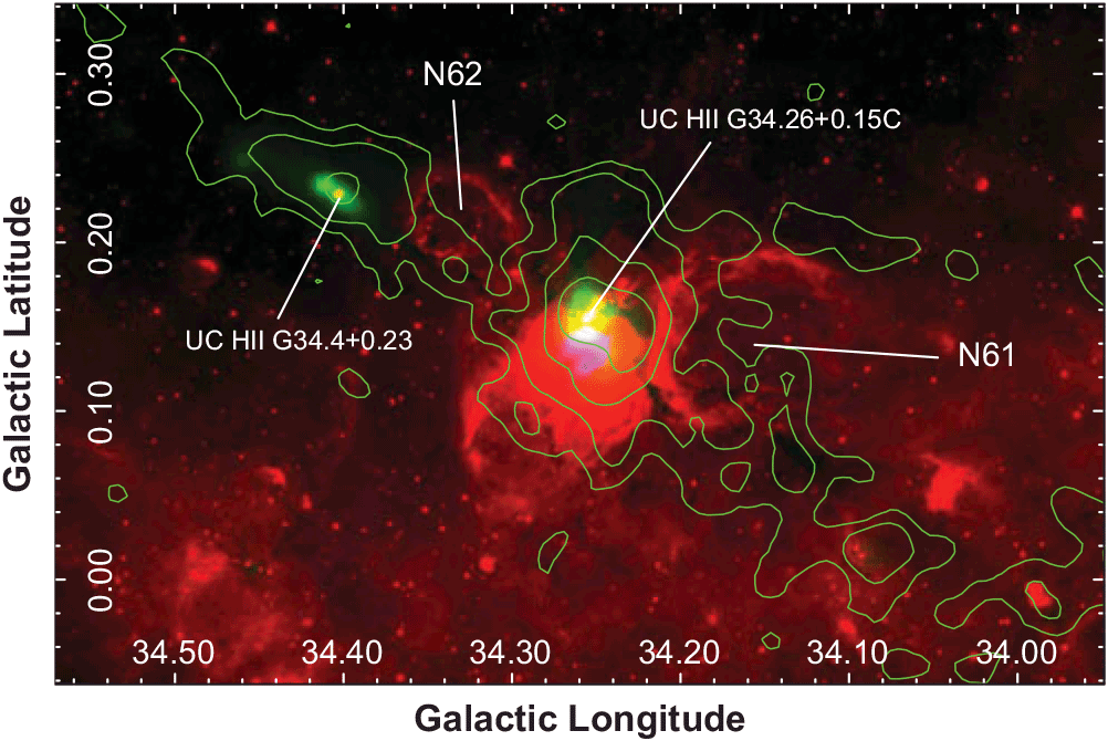
Figure 1. Three-colour image towards G34 complex displaying the Spitzer-IRAC 8-μm emission in red, the radio continuum emission at 20 cm as extracted from the MAGPIS in blue, and the continuum emission at 1.1 mm obtained from the Bolocam Survey in green. The green contours are the C18O J = 1–0 emission as presented in Figure 3 (bottom panel).
3. Data and the estimation of
$X^{13/18}$

3.1. Data
The 12CO, 13CO, and C18O J = 1–0 data were obtained from the FOREST unbiased Galactic plane imaging survey performed with the Nobeyama 45-m telescope (FUGIN project; Umemoto et al. Reference Umemoto2017)Footnote c. The angular resolutions are: 20 arcsec for the 12CO data, and 21 arcsec for the 13CO and C18O data. The spectral resolution is 1.3 km s–1 for all isotopes.
Graphical Astronomy and Image Analysis Tool (GAIA)Footnote d and tools from the Starlink software package (Currie et al. Reference Currie, Berry, Jenness, Gibb, Bell, Draper, Manset and Forshay2014) were used to analyse the data. Codes in python were developed to obtain the maps of the analysed parameters.
Additionally, we use IR data from the Hi-GAL survey (Molinari et al. Reference Molinari2010), retrieved from the Herschel Science ArchiveFootnote e. In particular, maps of Herschel-PACS at 70 and 160 μm (angular resolutions of about 6 and 12 arcsec, respectively), and maps of dust temperature and H2 column density derived from a SED fit between 70 and 500 μm (Marsh et al. Reference Marsh2017) were used (angular resolution of 36 arcsec).
3.2.
$X^{13/18}$
estimation

We carefully inspect the data cubes along the whole velocity range and find that the systemic velocity of the 13CO and C18O is quite homogeneous across the IRDC. The molecular emission extends from about 47 to 70 km s–1. Figure 2 displays average 12CO, 13CO, and C18O spectra towards the analysed region.
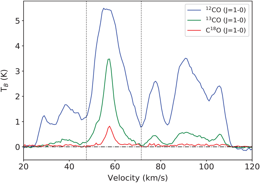
Figure 2. Average 12CO, 13CO, and C18O J = 1–0 spectra towards IRDC 34.43 + 0.24. The vertical dashed lines show the velocity range in which the IRDC extends.
In order to obtain maps of  $X^{13/18}$
(
$X^{13/18}$
( $X^{13/18}+\,=\,$
N(13CO)/N(C18O)), we need to calculate the 13CO and C18O column densities pixel-by-pixel. To do that, we assume local thermodynamic equilibrium (LTE) and a beam filling factor of 1, and we follow the standard procedures (e.g. Mangum & Shirley Reference Mangum and Shirley2015). The optical depths (
$X^{13/18}+\,=\,$
N(13CO)/N(C18O)), we need to calculate the 13CO and C18O column densities pixel-by-pixel. To do that, we assume local thermodynamic equilibrium (LTE) and a beam filling factor of 1, and we follow the standard procedures (e.g. Mangum & Shirley Reference Mangum and Shirley2015). The optical depths ( $\tau_{\rm ^{13}CO}$
and
$\tau_{\rm ^{13}CO}$
and  $\tau_{\rm C^{18}O}$
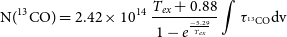
) and column densities (N(13CO) and N(C18O)) were derived from the following equations:
$\tau_{\rm C^{18}O}$
) and column densities (N(13CO) and N(C18O)) were derived from the following equations:
 \begin{gather}
\tau_{\rm ^{13}CO} = - ln\left(1 - \frac{T_{mb}({\rm ^{13}CO})}{5.29\left[\frac{1}{e^{5.29/T_{ex}}-1} - 0.164\right]}\right)\label{eqn1}\end{gather}
\begin{gather}
\tau_{\rm ^{13}CO} = - ln\left(1 - \frac{T_{mb}({\rm ^{13}CO})}{5.29\left[\frac{1}{e^{5.29/T_{ex}}-1} - 0.164\right]}\right)\label{eqn1}\end{gather}
 \begin{gather}
{\rm N(^{13}CO)} = 2.42 \times 10^{14}~\frac{T_{ex} + 0.88}{1 - e^{\frac{-5.29}{T_{ex}}}}
\int{\tau_{\rm ^{13}CO}{\rm dv}}
\label{eqn2}\end{gather}
\begin{gather}
{\rm N(^{13}CO)} = 2.42 \times 10^{14}~\frac{T_{ex} + 0.88}{1 - e^{\frac{-5.29}{T_{ex}}}}
\int{\tau_{\rm ^{13}CO}{\rm dv}}
\label{eqn2}\end{gather}
with
 \begin{gather}
\int{\tau_{\rm ^{13}CO}{\rm dv}} = \frac{1}{J(T_{ex}) - 0.868} \frac{\tau_{\rm ^{13}CO}}{1-e^{-\tau_{\rm ^{13}CO}}}
\int{T_{\rm mb}({\rm ^{13}CO}){\rm dv}}\label{eqn3}\end{gather}
\begin{gather}
\int{\tau_{\rm ^{13}CO}{\rm dv}} = \frac{1}{J(T_{ex}) - 0.868} \frac{\tau_{\rm ^{13}CO}}{1-e^{-\tau_{\rm ^{13}CO}}}
\int{T_{\rm mb}({\rm ^{13}CO}){\rm dv}}\label{eqn3}\end{gather}
 \begin{gather}
\tau_{\rm C^{18}O} = - ln\left(1 - \frac{T_{mb}({\rm C^{18}O})}{5.27\left[\frac{1}{e^{5.27/T_{ex}}-1} - 0.166\right]}\right)\label{eqn4}\end{gather}
\begin{gather}
\tau_{\rm C^{18}O} = - ln\left(1 - \frac{T_{mb}({\rm C^{18}O})}{5.27\left[\frac{1}{e^{5.27/T_{ex}}-1} - 0.166\right]}\right)\label{eqn4}\end{gather}
 \begin{gather}
{\rm N(C^{18}O)} = 2.42 \times 10^{14}~\frac{T_{ex} + 0.88}{1 - e^{\frac{-5.27}{T_{ex}}}}
\int{\tau_{\rm C^{18}O}{\rm dv}}
\label{eqn5}\end{gather}
\begin{gather}
{\rm N(C^{18}O)} = 2.42 \times 10^{14}~\frac{T_{ex} + 0.88}{1 - e^{\frac{-5.27}{T_{ex}}}}
\int{\tau_{\rm C^{18}O}{\rm dv}}
\label{eqn5}\end{gather}
with
 \begin{equation}
\int{\tau_{\rm C^{18}O}{\rm dv}} = \frac{1}{J(T_{ex}) - 0.872} \frac{\tau_{\rm C^{18}O}}{1-e^{-\tau_{\rm C^{18}O}}}
\int{T_{\rm mb}({\rm C^{18}O}){\rm dv}}
\label{eqn6}
\end{equation}
\begin{equation}
\int{\tau_{\rm C^{18}O}{\rm dv}} = \frac{1}{J(T_{ex}) - 0.872} \frac{\tau_{\rm C^{18}O}}{1-e^{-\tau_{\rm C^{18}O}}}
\int{T_{\rm mb}({\rm C^{18}O}){\rm dv}}
\label{eqn6}
\end{equation}
in which correction for high optical depths was applied (Frerking et al. Reference Frerking, Langer and Wilson1982). This correction is indeed required in the case of 13CO but not for C18O because it is mostly optically thin.
The  $J(T_{ex})$
parameter is
$J(T_{ex})$
parameter is  $\frac{5.29}{exp(\frac{5.29}{T_{ex}}) - 1}$
and
$\frac{5.29}{exp(\frac{5.29}{T_{ex}}) - 1}$
and  $\frac{5.27}{exp(\frac{5.27}{T_{ex}}) - 1}$
for equations (3) and (6), respectively.
$\frac{5.27}{exp(\frac{5.27}{T_{ex}}) - 1}$
for equations (3) and (6), respectively.  $T_{\rm mb}$
and
$T_{\rm mb}$
and  $T_{ex}$
are the main brightness temperature and the excitation temperature, respectively. Assuming that the 12CO J = 1–0 emission is optically thick, it is possible to derive
$T_{ex}$
are the main brightness temperature and the excitation temperature, respectively. Assuming that the 12CO J = 1–0 emission is optically thick, it is possible to derive  $T_{ex}$
from:
$T_{ex}$
from:
 \begin{equation}
T_{ex} = \frac{5.53}{{\rm ln}[1 + 5.53 / (^{12}T_{\rm peak} + 0.818)]}
\label{eqn7}
\end{equation}
\begin{equation}
T_{ex} = \frac{5.53}{{\rm ln}[1 + 5.53 / (^{12}T_{\rm peak} + 0.818)]}
\label{eqn7}
\end{equation}
where  $^{12}T_{\rm peak}$
is the 12CO peak temperature. Thus from maps of
$^{12}T_{\rm peak}$
is the 12CO peak temperature. Thus from maps of  $^{12}T_{\rm peak}$
, maps of excitation temperatures (
$^{12}T_{\rm peak}$
, maps of excitation temperatures ( $T_{ex}$
) are obtained. Before obtaining the column densities maps, we generate 13CO and C18O optical depths (
$T_{ex}$
) are obtained. Before obtaining the column densities maps, we generate 13CO and C18O optical depths ( $\tau^{13}$
and
$\tau^{13}$
and  $\tau^{18}$
) maps and check the values.
$\tau^{18}$
) maps and check the values.
In some pixels, we notice that  $\tau^{13}$
becomes undefined due to a negative argument in the logarithm of Equation 1. It is likely that this issue is a consequence of high saturation in the line emission. We investigate the spectra corresponding to such pixels and we find that the 12CO profiles indeed present signs of saturation and self-absorption which may affect the estimate of Tex. Also some 13CO spectra in such pixels, and in others, mainly at the vicinity of the UC G34.26 + 0.15C, present kinematic signatures of infall (as found by Xu et al. Reference Xu, Li, Zhang, Liu, Wang, Ning and Ju2016) that prevent us to obtain reliable values of column densities.
$\tau^{13}$
becomes undefined due to a negative argument in the logarithm of Equation 1. It is likely that this issue is a consequence of high saturation in the line emission. We investigate the spectra corresponding to such pixels and we find that the 12CO profiles indeed present signs of saturation and self-absorption which may affect the estimate of Tex. Also some 13CO spectra in such pixels, and in others, mainly at the vicinity of the UC G34.26 + 0.15C, present kinematic signatures of infall (as found by Xu et al. Reference Xu, Li, Zhang, Liu, Wang, Ning and Ju2016) that prevent us to obtain reliable values of column densities.
4. Results
4.1. Molecular gas
Figure 3 displays the molecular gas distribution associated with the IRDC 34.43 + 0.24 in the 13CO and C18O J=1–0 line integrated between 47 and 70 km s–1, with an angular resolution of 21 arcsec. The lowest contour of the integrated C18O is 4 $\sigma$
. We consider it as a threshold to study the abundance ratio and others physical parameters derived in this work, that is, all the analyses are done for the region contained by this C18O contour.
$\sigma$
. We consider it as a threshold to study the abundance ratio and others physical parameters derived in this work, that is, all the analyses are done for the region contained by this C18O contour.
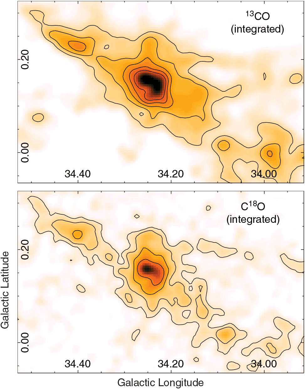
Figure 3. Top and bottom panels: maps showing the 13CO and C18O J = 1–0 line integrated between 47 and 70 km s–1, respectively. The contours levels are 22, 30, 40, 50, and 60 K km s–1, and 4, 6, 10, and 16 K km s–1 for the 13CO and C18O, respectively. The angular resolution is 21 arcsec. The sigma levels of these integrated maps are  $\sigma_{13} = 4.5$
and
$\sigma_{13} = 4.5$
and  $\sigma_{18} = 1.0$
K km s–1.
$\sigma_{18} = 1.0$
K km s–1.
Figure 4 shows a map of the excitation temperature obtained from the 12CO J = 1–0 emission following equation (7), and Figure 5 displays the maps of the obtained 13CO and C18O optical depths. Figure 6 presents the obtained maps of the 13CO and C18O column densities and the derived abundance ratio  $X^{13/18}$
. Figure 7 shows the integrated line ratio (
$X^{13/18}$
. Figure 7 shows the integrated line ratio (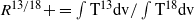 $R^{13/18}+=\int{\rm T^{13}dv}/\int{\rm T^{18}dv}$
), and Table 1 presents ranges and averages values of the physical parameters obtained from our analysis.
$R^{13/18}+=\int{\rm T^{13}dv}/\int{\rm T^{18}dv}$
), and Table 1 presents ranges and averages values of the physical parameters obtained from our analysis.

Figure 4. Excitation temperature map derived from the 12CO J = 1–0 emission in the region of the C18O emission. For reference, the C18O contours presented in Figure 3 (bottom panel) are included.
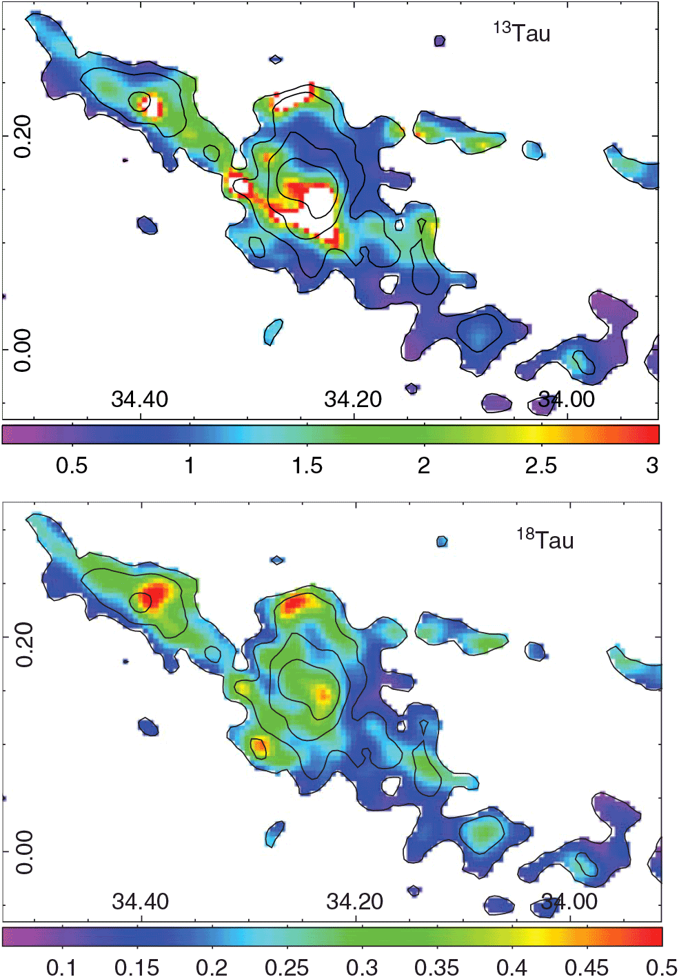
Figure 5. Maps showing the 13CO and C18O optical depths (top and bottom panels, respectively). Contours of the integrated C18O J = 1–0 emission are included for reference.
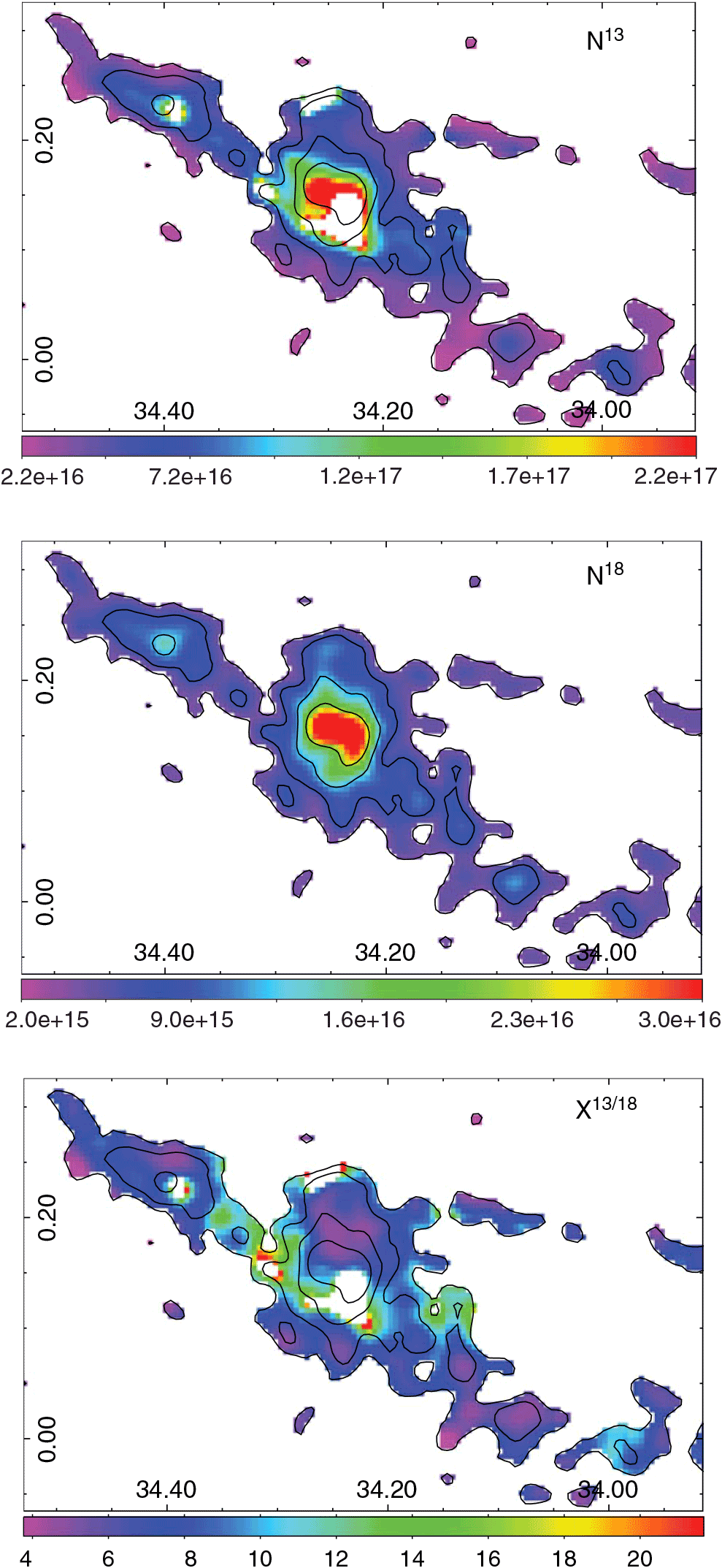
Figure 6. Top and middle panels: maps showing the 13CO and C18O column densities, respectively. The colourbars are in units of cm–2. Bottom panel: the abundance ratio  $X^{13/18}$
. Contours of the integrated C18O J = 1–0 emission are included for reference.
$X^{13/18}$
. Contours of the integrated C18O J = 1–0 emission are included for reference.
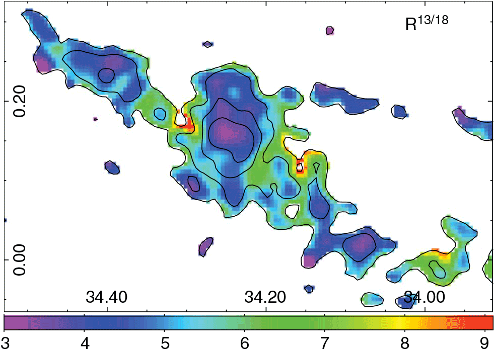
Figure 7. Integrated line ratio ( $R^{13/18}$
). Contours of the integrated C18O J = 1–0 emission are included for reference.
$R^{13/18}$
). Contours of the integrated C18O J = 1–0 emission are included for reference.
Table 1. Ranges of physical parameters.
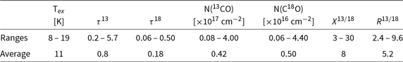
Figure 8 shows the relation between the abundance ratio  $X^{13/18}$
and the integrated line ratio
$X^{13/18}$
and the integrated line ratio  $R^{13/18}$
obtained from different sectors of the molecular cloud defined by the C18O contours: Region A (pixels lying between the contours at 4 and 6 K km s–1), Region B (pixels between contours 6 and 10 K km s–1), Region C (pixels between contours 10 and 16 K km s–1), and Region D (pixels within the contour at 16 K km s–1). The slopes (m) and correlations factors (r) from linear fittings for each case are included in the figure.
$R^{13/18}$
obtained from different sectors of the molecular cloud defined by the C18O contours: Region A (pixels lying between the contours at 4 and 6 K km s–1), Region B (pixels between contours 6 and 10 K km s–1), Region C (pixels between contours 10 and 16 K km s–1), and Region D (pixels within the contour at 16 K km s–1). The slopes (m) and correlations factors (r) from linear fittings for each case are included in the figure.
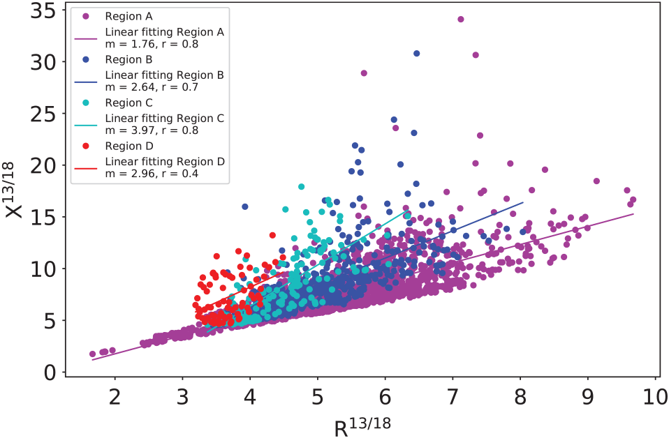
Figure 8. Abundance ratio ( $X^{13/18}$
) vs. integrated line ratio (
$X^{13/18}$
) vs. integrated line ratio ( $R^{13/18}$
). Region A, B, and C correspond to pixels between the C18O J = 1–0 contours 4 and 6, 6 and 10, and 10 and 16 K km s–1, respectively, and Region D corresponds to pixels within the 16 K km s–1 C18O contour. Slopes (m) and correlations factors (r) from linear fittings are included.
$R^{13/18}$
). Region A, B, and C correspond to pixels between the C18O J = 1–0 contours 4 and 6, 6 and 10, and 10 and 16 K km s–1, respectively, and Region D corresponds to pixels within the 16 K km s–1 C18O contour. Slopes (m) and correlations factors (r) from linear fittings are included.
4.2. Determining the FUV radiation field
Given that the clouds seen in far-IR (FIR) are mainly heated by FUV radiation, it is possible to estimate the FUV radiation field from the observed FIR intensity ( $I_{FIR}$
) (see Kramer et al. Reference Kramer2008). We compute the FUV radiation field from the FIR intensity in the 60–200 μm range using the Herschel-PACS 70- and 160-μm maps. These maps were convolved to the resolution of the molecular data, and following the procedure explained in Roccatagliata et al. (Reference Roccatagliata, Preibisch, Ratzka and Gaczkowski2013), we generate the FUV radiation map in units of the Habing field from:
$I_{FIR}$
) (see Kramer et al. Reference Kramer2008). We compute the FUV radiation field from the FIR intensity in the 60–200 μm range using the Herschel-PACS 70- and 160-μm maps. These maps were convolved to the resolution of the molecular data, and following the procedure explained in Roccatagliata et al. (Reference Roccatagliata, Preibisch, Ratzka and Gaczkowski2013), we generate the FUV radiation map in units of the Habing field from:
 \begin{equation}
G_{0} = \frac{4 \pi I_{FIR}}{1.6 \times 10^{-3}~{\rm erg~cm^{-2}~s^{-1}}},
\label{eqn8}
\end{equation}
\begin{equation}
G_{0} = \frac{4 \pi I_{FIR}}{1.6 \times 10^{-3}~{\rm erg~cm^{-2}~s^{-1}}},
\label{eqn8}
\end{equation}
which is presented in Figure 9. Besides, in Figure 10, we present the same FUV radiation field towards the centre of the analysed region where the UC H ii region G34.26+0.15C and the radio continuum shell lie. To do this map with the best angular resolution as possible, the image of PACS 70 μm was convolved to the angular resolution of the PACS 160-μm map (about 12 arcsec), and the same procedure done for the map of Figure 9 was applied. Contours of the radio continuum emission are included to analyse the ionised gas component in relation to the FUV radiation.
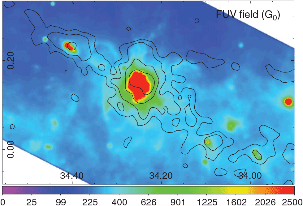
Figure 9. Far ultraviolet flux G0 in units of Habing field. The angular resolution of the image is 21 arcsec. Contours of the integrated C18O J = 1–0 emission are included for reference.

Figure 10. Far ultraviolet flux G0 in units of Habing field towards the centre of the analysed region. The angular resolution of the image is about 12 arcsec. Contours of the radio continuum emission at 20 cm are presented with levels of 0.02, 0.05, 0.10, 0.15, and 0.20 Jy beam–1.
4.3. Tdust and N(H2) towards the centre of the IRDC
To make comparisons between the emissions of the molecular gas and the dust, we obtain mapsFootnote f of the dust temperature and H2 column density N(H2) (see Figure 11) which were generated from the PPMAP procedure done to the Hi-GAL maps in the wavelength range 70–500 μm (Marsh et al. Reference Marsh2017).
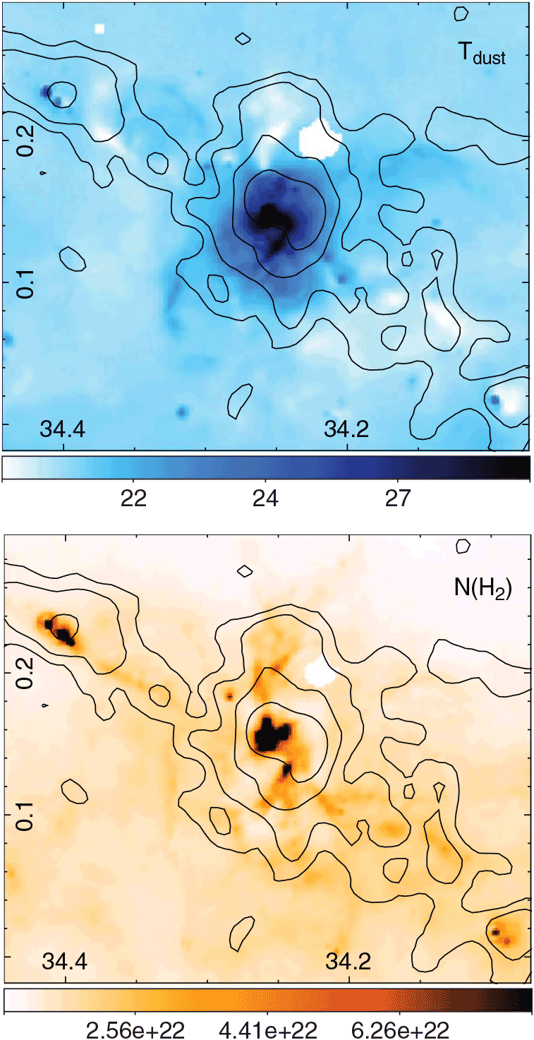
Figure 11. Maps of dust temperature (top) and H2 column density (bottom) obtained from http://www.astro.cardiff.ac.uk/research/ViaLactea/. The colourbars are in units of K and cm–2, respectively. Contours of the integrated C18O J = 1–0 are presented for reference.
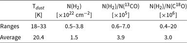
Ranges of dust temperature (Tdust) and N(H2) with the average values are presented in Table 2. Additionally, after convolving the N(13CO) and N(C18O) maps to the angular resolution of the N(H2) map (about 36 arcsec), we generate maps of N(H2)/N(13CO) and N(H2)/N(C18O) (see Figure 12) whose ranges and average values are also presented in Table 2.
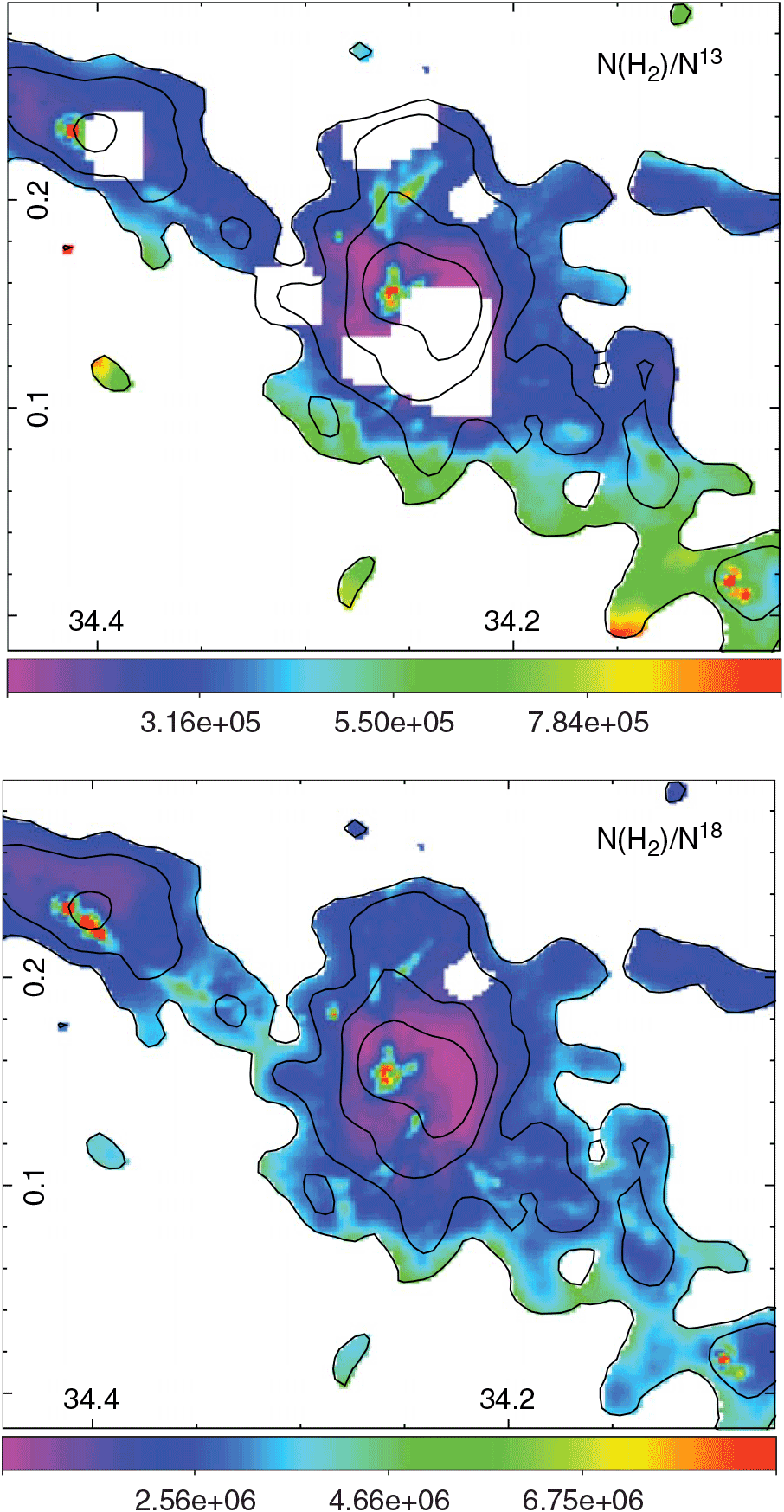
Figure 12. Maps of N(H2)/N(13CO) and N(H2)/N(C18O). The angular resolution of these maps is about 36 arcsec. Contours of the integrated C18O J = 1–0 are presented for reference.
Table 2. Parameters derived from the IR data.
To investigate the dependence of  $X^{13/18}$
on the visual extinction towards this IRDC, we obtain an AV map from the N(H2) following the relation from Bohlin et al. (Reference Bohlin, Savage and Drake1978)
$X^{13/18}$
on the visual extinction towards this IRDC, we obtain an AV map from the N(H2) following the relation from Bohlin et al. (Reference Bohlin, Savage and Drake1978)
 \begin{equation}
A_{\rm V} = \frac{\rm N(H_{2})}{9.4 \times 10^{20} {\rm cm^{-2}}}.
\label{eqn9}
\end{equation}
\begin{equation}
A_{\rm V} = \frac{\rm N(H_{2})}{9.4 \times 10^{20} {\rm cm^{-2}}}.
\label{eqn9}
\end{equation}
The map of  $X^{13/18}$
was convolved to the angular resolution of the AV map and in Figure 13 we present plots of
$X^{13/18}$
was convolved to the angular resolution of the AV map and in Figure 13 we present plots of  $X^{13/18}$
vs. AV.
$X^{13/18}$
vs. AV.
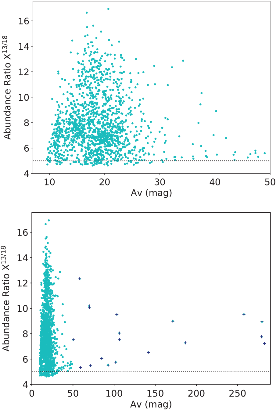
Figure 13. Correlation between  $X^{13/18}$
and the visual absorption AV up to AV = 50 mag (top panel) and along the whole AV range (bottom panel). In bottom panel, the points corresponding to pixels at the positions of the UC H ii regions and their close surroundings are marked with blue crosses.
$X^{13/18}$
and the visual absorption AV up to AV = 50 mag (top panel) and along the whole AV range (bottom panel). In bottom panel, the points corresponding to pixels at the positions of the UC H ii regions and their close surroundings are marked with blue crosses.
5. Discussion
The molecular emission extends along the whole filamentary structure of IRDC 34.43 + 0.24, and as shown in Figure 3, the morphology of the C18O emission is narrower and fits better with the infrared emission from IRDC than the 13CO one. The ranges of N(13CO), N(C18O), and  $X^{13/18}$
are quite similar to those found towards the Orion-A giant molecular cloud by Shimajiri et al. (Reference Shimajiri2014). Additionally, our range of values of
$X^{13/18}$
are quite similar to those found towards the Orion-A giant molecular cloud by Shimajiri et al. (Reference Shimajiri2014). Additionally, our range of values of  $X^{13/18}$
also is in agreement with those values found towards LDN 1551, a nearby and isolated star-forming region (Lin et al. Reference Lin2016). Thus, our results show that
$X^{13/18}$
also is in agreement with those values found towards LDN 1551, a nearby and isolated star-forming region (Lin et al. Reference Lin2016). Thus, our results show that  $X^{13/18}$
may have a similar behaviour among regions that are located at very different distances from us. The obtained
$X^{13/18}$
may have a similar behaviour among regions that are located at very different distances from us. The obtained  $X^{13/18}$
average value (about 8) across the IRDC is larger than the solar system value of 5.5.
$X^{13/18}$
average value (about 8) across the IRDC is larger than the solar system value of 5.5.
Assuming a distance of 3.9 kpc to IRDC 34.43 + 0.24, a galactocentric distance of about 5.7 kpc is obtained, and following the relation between atomic ratios and the galactocentric distance presented in Wilson & Rood (Reference Wilson and Rood1994), a  $X^{13/18}$
of 7.4 is derived. While this value is in quite agreement with our average value of
$X^{13/18}$
of 7.4 is derived. While this value is in quite agreement with our average value of  $X^{13/18}$
, it does not reflect the wide range of values found across the molecular cloud. Therefore, it is important to remark that assuming the ‘canonical’
$X^{13/18}$
, it does not reflect the wide range of values found across the molecular cloud. Therefore, it is important to remark that assuming the ‘canonical’  $X^{13/18}$
from Wilson & Rood (Reference Wilson and Rood1994) may introduce some bias in the analysis of the molecular gas, mainly in regions that are exposed to FUV radiation.
$X^{13/18}$
from Wilson & Rood (Reference Wilson and Rood1994) may introduce some bias in the analysis of the molecular gas, mainly in regions that are exposed to FUV radiation.
Figure 6 (bottom panel) shows that highest values in  $X^{13/18}$
are found towards regions related to the interiors and/or borders of N61 and N62 bubbles. This can be explained through selective photodissociation of the C18O molecule due to the radiation responsible for the bubbles generation, which may represents an observational support to the C18O selectively photodissociation phenomenon, as found towards other nearby galactic regions (e.g. Yamagishi et al. Reference Yamagishi2019; Lin et al. Reference Lin2016; Kong et al. Reference Kong, Lada, Lada, Román-Zúñiga, Bieging, Lombardi, Forbrich and Alves2015) but in a quite distant filamentary IRDC. In general, an increase in
$X^{13/18}$
are found towards regions related to the interiors and/or borders of N61 and N62 bubbles. This can be explained through selective photodissociation of the C18O molecule due to the radiation responsible for the bubbles generation, which may represents an observational support to the C18O selectively photodissociation phenomenon, as found towards other nearby galactic regions (e.g. Yamagishi et al. Reference Yamagishi2019; Lin et al. Reference Lin2016; Kong et al. Reference Kong, Lada, Lada, Román-Zúñiga, Bieging, Lombardi, Forbrich and Alves2015) but in a quite distant filamentary IRDC. In general, an increase in  $X^{13/18}$
is observed near the PDRs (see the 8-μm emission in Figure 1), precisely the regions in which FUV photons are interacting with the molecular gas. From the FIR intensity, we estimate the FUV radiation field, which mainly reflects the action of the FUV photons in the dust. An increase in the FUV radiation field is observed towards the G34 complex, where the UC H ii region G34.26 + 0.15C lies, and towards the position of UC H ii region G34.4 + 0.23 at the north-east of the IRDC (see Figure 9). By comparing the FUV map with the
$X^{13/18}$
is observed near the PDRs (see the 8-μm emission in Figure 1), precisely the regions in which FUV photons are interacting with the molecular gas. From the FIR intensity, we estimate the FUV radiation field, which mainly reflects the action of the FUV photons in the dust. An increase in the FUV radiation field is observed towards the G34 complex, where the UC H ii region G34.26 + 0.15C lies, and towards the position of UC H ii region G34.4 + 0.23 at the north-east of the IRDC (see Figure 9). By comparing the FUV map with the  $X^{13/18}$
map, two possible aspects of the influence of the UC H ii regions in the abundance ratio can be inferred: in clumps far from the UC H ii regions, some
$X^{13/18}$
map, two possible aspects of the influence of the UC H ii regions in the abundance ratio can be inferred: in clumps far from the UC H ii regions, some  $X^{13/18}$
minimums coincide with C18O maximums, while in regions related to the clumps where the UC H ii regions are embedded, this correlation is broken. It is likely that the dust (which reflects the FUV field) may shield the molecular gas, and hence it is not possible to analyse a direct correlation between the
$X^{13/18}$
minimums coincide with C18O maximums, while in regions related to the clumps where the UC H ii regions are embedded, this correlation is broken. It is likely that the dust (which reflects the FUV field) may shield the molecular gas, and hence it is not possible to analyse a direct correlation between the  $X^{13/18}$
factor and the FUV radiation field derived from the FIR emission.
$X^{13/18}$
factor and the FUV radiation field derived from the FIR emission.
From a comparison between the radio continuum emission and the FUV radiation field (Figure 10), it is worth noting that the observed radio continuum shell, which represents ionised gas due to Lyman photons, is surrounded by the FUV radiation field, showing the typical stratification of a PDR in H ii regions (e.g. Draine Reference Draine2011).
By comparing the maps of  $X^{13/18}$
and
$X^{13/18}$
and  $R^{13/18}$
, that is, comparing values that were derived from the LTE assumption with values from direct measurements, a quite similar behaviour can be appreciated across the region. The plot
$R^{13/18}$
, that is, comparing values that were derived from the LTE assumption with values from direct measurements, a quite similar behaviour can be appreciated across the region. The plot  $X^{13/18}$
vs.
$X^{13/18}$
vs.  $R^{13/18}$
shows a linear tendency with an increase in the slope as we analyse more dense regions in the cloud (see Figure 8). This behaviour may be explained by a major increase in
$R^{13/18}$
shows a linear tendency with an increase in the slope as we analyse more dense regions in the cloud (see Figure 8). This behaviour may be explained by a major increase in  $\tau^{13}$
with respect to
$\tau^{13}$
with respect to  $\tau^{18}$
. On the other side, Region D shows a low correlation factor, which may be due to that in this region some 13CO spectra present kinematic signatures of infall, and thus, the LTE assumption would no longer be valid in some pixels corresponding to it.
$\tau^{18}$
. On the other side, Region D shows a low correlation factor, which may be due to that in this region some 13CO spectra present kinematic signatures of infall, and thus, the LTE assumption would no longer be valid in some pixels corresponding to it.
Assuming that the gas and dust are coupled, we can compare the 13CO and C18O column densities obtained from the molecular lines with the N(H2) derived from the dust emission. The obtained average ratio N(H2)/N(13CO) of about  $4\times10^{5}$
is in close agreement with the typical abundance ratio extensively used in the literature (N(H2)/N(13CO)
$4\times10^{5}$
is in close agreement with the typical abundance ratio extensively used in the literature (N(H2)/N(13CO) $=5\times10^{5}$
, e.g. Pineda et al. Reference Pineda, Caselli and Goodman2008, and references therein). The average ratio N(H2)/N(C18O) of
$=5\times10^{5}$
, e.g. Pineda et al. Reference Pineda, Caselli and Goodman2008, and references therein). The average ratio N(H2)/N(C18O) of  $3.0\times10^{6}$
obtained in this work is in quite agreement with the typical [H2]/[C18O] ratio (
$3.0\times10^{6}$
obtained in this work is in quite agreement with the typical [H2]/[C18O] ratio ( $5.8\times10^{6}$
, e.g. Frerking et al. Reference Frerking, Langer and Wilson1982).
$5.8\times10^{6}$
, e.g. Frerking et al. Reference Frerking, Langer and Wilson1982).
Additionally, we compare  $X^{13/18}$
with the visual absorption AV derived from N(H2). The maximum in
$X^{13/18}$
with the visual absorption AV derived from N(H2). The maximum in  $X^{13/18}$
occurs between 17 and 22 mag, and the behaviour of this relation is similar as found in previous works (e.g. Kong et al. Reference Kong, Lada, Lada, Román-Zúñiga, Bieging, Lombardi, Forbrich and Alves2015; Kim et al. Reference Kim, Kim, Lee, Minh, Balasubramanyam, Burton, Millar and Lee2006; Lada et al. Reference Lada, Lada, Clemens and Bally1994). In our case, an increase in
$X^{13/18}$
occurs between 17 and 22 mag, and the behaviour of this relation is similar as found in previous works (e.g. Kong et al. Reference Kong, Lada, Lada, Román-Zúñiga, Bieging, Lombardi, Forbrich and Alves2015; Kim et al. Reference Kim, Kim, Lee, Minh, Balasubramanyam, Burton, Millar and Lee2006; Lada et al. Reference Lada, Lada, Clemens and Bally1994). In our case, an increase in  $X^{13/18}$
with respect to AV can be inferred towards the highest AV values. We conclude that this plot shows selective photodissociation generated by both, external radiation (probably from the interstellar radiation field (Lin et al. Reference Lin2016), and/or radiation from surrounding sources such as bubbles N61 and N62) and radiation from deeply embedded sources such as the UC H ii regions.
$X^{13/18}$
with respect to AV can be inferred towards the highest AV values. We conclude that this plot shows selective photodissociation generated by both, external radiation (probably from the interstellar radiation field (Lin et al. Reference Lin2016), and/or radiation from surrounding sources such as bubbles N61 and N62) and radiation from deeply embedded sources such as the UC H ii regions.
5.1. Beam filling factor effects and clumpiness
It is known that the clouds are highly structured on the subparsec scale implying beam filling factors less than the unity. We investigate the influence of a possible beam dilution effect in the  $X^{13/18}$
. The beam filling factor can be estimated from (Kim et al. Reference Kim, Kim, Lee, Minh, Balasubramanyam, Burton, Millar and Lee2006):
$X^{13/18}$
. The beam filling factor can be estimated from (Kim et al. Reference Kim, Kim, Lee, Minh, Balasubramanyam, Burton, Millar and Lee2006): 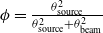 $\phi=\frac{\theta^2_{\rm source}}{\theta^2_{\rm source}+\theta^2_{\rm beam}}$
where
$\phi=\frac{\theta^2_{\rm source}}{\theta^2_{\rm source}+\theta^2_{\rm beam}}$
where  $\theta^2_{\rm source}$
and
$\theta^2_{\rm source}$
and  $\theta^2_{\rm beam}$
are the source and beam sizes, respectively. The beam size of 13CO and C18O J = 1–0 data is 20 arcsec, which corresponds to 0.37 pc at the distance of 3.9 kpc. From the emission with the best angular resolution used in this work, that is, Herschel-PACS 70 μm (angular resolution ∼5 arcsec), we determine that the sizes of clumps in the region are expected to exceed 0.7 pc. Thus, the beam filling factor of the used molecular data is expected to exceed 0.4. Given that the 13CO traces more extended molecular components than the C18O, we consider the limit case in which
$\theta^2_{\rm beam}$
are the source and beam sizes, respectively. The beam size of 13CO and C18O J = 1–0 data is 20 arcsec, which corresponds to 0.37 pc at the distance of 3.9 kpc. From the emission with the best angular resolution used in this work, that is, Herschel-PACS 70 μm (angular resolution ∼5 arcsec), we determine that the sizes of clumps in the region are expected to exceed 0.7 pc. Thus, the beam filling factor of the used molecular data is expected to exceed 0.4. Given that the 13CO traces more extended molecular components than the C18O, we consider the limit case in which  $\phi_{^{13}{\rm CO}}=1$
and
$\phi_{^{13}{\rm CO}}=1$
and  $\phi_{\rm C^{18}O}=0.4$
. Thus,
$\phi_{\rm C^{18}O}=0.4$
. Thus,  $X^{13/18}$
could be overestimated up to 60%.
$X^{13/18}$
could be overestimated up to 60%.
Taking into account that the beam dilution effect would be more important towards the densest/clumpy regions (mainly traced by the C18O emission) than in regions with diffuse gas, the actual  $X^{13/18}$
value should be smaller than the measured one in clumpy regions. This is in agreement with Zielinsky et al. (Reference Zielinsky, Stutzki and Störzer2000), who point out that as the C18O emitting regions have much smaller extent than the 13CO ones, resulting in a lower area filling factor, and also lower temperatures, larger (i.e. overestimated)
$X^{13/18}$
value should be smaller than the measured one in clumpy regions. This is in agreement with Zielinsky et al. (Reference Zielinsky, Stutzki and Störzer2000), who point out that as the C18O emitting regions have much smaller extent than the 13CO ones, resulting in a lower area filling factor, and also lower temperatures, larger (i.e. overestimated)  $X^{13/18}$
values may be observed. Anyway, if the beam dilution is considered in these regions, the behaviour of
$X^{13/18}$
values may be observed. Anyway, if the beam dilution is considered in these regions, the behaviour of  $X^{13/18}$
across the whole IRDC would highlight even more the effects of the selective photodissociation.
$X^{13/18}$
across the whole IRDC would highlight even more the effects of the selective photodissociation.
6. Conclusions
We carried out a large-scale analysis of the abundance ratio  $X^{13/18}$
along the filamentary IRDC 34.43 + 0.24 using the 12CO, 13CO, and 13CO J = 1–0 emission with an angular resolution of about 20 arcsec.
$X^{13/18}$
along the filamentary IRDC 34.43 + 0.24 using the 12CO, 13CO, and 13CO J = 1–0 emission with an angular resolution of about 20 arcsec.
In the line of previous works towards relative nearby molecular clouds, we find strong observational evidences supporting the C18O selectively photodissociation due to the FUV photons in a quite distance filamentary IRDC. A range of  $X^{13/18}$
between 3 and 30 was found across the molecular cloud related to the IRDC, with an average value of 8, larger than the typical solar value of about 5. From the FIR intensity, we estimate the FUV radiation field, which mainly reflects the action of the FUV photons in the dust. We conclude that it is not possible to analyse a direct correlation between the
$X^{13/18}$
between 3 and 30 was found across the molecular cloud related to the IRDC, with an average value of 8, larger than the typical solar value of about 5. From the FIR intensity, we estimate the FUV radiation field, which mainly reflects the action of the FUV photons in the dust. We conclude that it is not possible to analyse a direct correlation between the  $X^{13/18}$
and the FUV radiation field derived from the FIR emission because it is likely that in some regions the dust may shield the molecular gas from the FUV photons.
$X^{13/18}$
and the FUV radiation field derived from the FIR emission because it is likely that in some regions the dust may shield the molecular gas from the FUV photons.
From a comparison between  $X^{13/18}$
and the visual absorption AV, we conclude that selective photodissociation can be generated by both the interstellar radiation field and/or radiation from surrounding H ii regions (i.e. external radiation), and radiation from deeply embedded sources in the IRDC.
$X^{13/18}$
and the visual absorption AV, we conclude that selective photodissociation can be generated by both the interstellar radiation field and/or radiation from surrounding H ii regions (i.e. external radiation), and radiation from deeply embedded sources in the IRDC.
The average values of  $X^{13/18}$
, N(H2)/N(13CO), and N(H2)/N(C18O), in which the N(H2) was independently estimated from the dust emission, are in quite agreement with the ‘canonical’ values used in the literature. However, works like this show that if an accurate analysis of the molecular gas is required, the use of these ‘canonical’ values may introduce some bias. In those cases, how the gas is irradiated by FUV photons and the implications of beam dilution should be considered, which can affect in different ways the abundance ratios.
$X^{13/18}$
, N(H2)/N(13CO), and N(H2)/N(C18O), in which the N(H2) was independently estimated from the dust emission, are in quite agreement with the ‘canonical’ values used in the literature. However, works like this show that if an accurate analysis of the molecular gas is required, the use of these ‘canonical’ values may introduce some bias. In those cases, how the gas is irradiated by FUV photons and the implications of beam dilution should be considered, which can affect in different ways the abundance ratios.
Acknowledgements
We thank the anonymous referee for her/his very helpful comments and suggestions. M.B.A. and L.D. are doctoral fellows of CONICET, Argentina. S.P. and M.O. are members of the Carrera del Investigador Científico of CONICET, Argentina. This work was partially supported by Argentina grants awarded by UBA (UBACyT) and ANPCYT. Nobeyama Radio Observatory is a branch of the National Astronomical Observatory of Japan, National Institutes of Natural Sciences.


