


1. Introduction
The study of the first luminous sources has remained at the forefront of astrophysics for more than a decade. The radiation emitted from these sources, re-ionised the Universe and marked a pivotal transition period in the early Universe. Exploring this period is, therefore, valuable in understanding the evolution of the early Universe. Observational cosmology employs various methods to explore the cosmic history of the early Universe. One powerful approach is the study of the Lyman-alpha (Ly
 $\alpha$
) forests, which provide valuable insights into the ionisation and temperature of the intergalactic medium (IGM) at the end of the Epoch of Reionisation (EoR) (Morales & Wyithe Reference Morales and Wyithe2010; Furlanetto Reference Furlanetto and Mesinger2016). Complementary techniques include galaxy surveys for understanding high redshift galaxies (Tang et al. Reference Tang2023; Bunker et al. Reference Bunker2023) and Cosmic Microwave Background (CMB) radiation (Planck Collaboration et al. 2016). These methods offer glimpses into the properties of the ionising sources and the reionisation history. However, these existing techniques have limitations, and therefore, observational cosmology requires a new probe to study the early Universe consisting of the Dark Age, the Cosmic Dawn and the EoR. The 21 cm cosmological signal of the neutral hydrogen is a potential probe in studying the early Universe (Furlanetto, Oh, & Briggs Reference Furlanetto, Oh and Briggs2006; Pritchard & Loeb Reference Pritchard and Loeb2012). The brightness temperature fluctuations of the redshifted 21 cm signal is used to trace the three-dimensional evolution of the early Universe.
$\alpha$
) forests, which provide valuable insights into the ionisation and temperature of the intergalactic medium (IGM) at the end of the Epoch of Reionisation (EoR) (Morales & Wyithe Reference Morales and Wyithe2010; Furlanetto Reference Furlanetto and Mesinger2016). Complementary techniques include galaxy surveys for understanding high redshift galaxies (Tang et al. Reference Tang2023; Bunker et al. Reference Bunker2023) and Cosmic Microwave Background (CMB) radiation (Planck Collaboration et al. 2016). These methods offer glimpses into the properties of the ionising sources and the reionisation history. However, these existing techniques have limitations, and therefore, observational cosmology requires a new probe to study the early Universe consisting of the Dark Age, the Cosmic Dawn and the EoR. The 21 cm cosmological signal of the neutral hydrogen is a potential probe in studying the early Universe (Furlanetto, Oh, & Briggs Reference Furlanetto, Oh and Briggs2006; Pritchard & Loeb Reference Pritchard and Loeb2012). The brightness temperature fluctuations of the redshifted 21 cm signal is used to trace the three-dimensional evolution of the early Universe.
The datasets of 21 cm experiments are dominated by foregrounds, three to four orders of magnitude greater than the weak cosmological signal (Shaver et al. Reference Shaver, Windhorst, Madau and de Bruyn1999; Di Matteo et al. Reference Di Matteo, Perna, Abel and Rees2002; Di Matteo, Ciardi, & Miniati Reference Di Matteo, Ciardi and Miniati2004). Additionally, the existing 21 cm experiments lack the necessary sensitivity to make the detection in image space. Therefore, these experiments instead aim to statistically detect the signal using the power spectrum. The power spectrum measures the signal variance, which encodes most of the cosmological information. The 21 cm signal is homogeneous and isotropic, hence, in the Fourier space, the signal is spherically symmetric (Morales & Hewitt Reference Morales and Hewitt2004; Morales, Bowman, & Hewitt Reference Morales, Bowman and Hewitt2006). Thus, all the observations within a given spherical shell can be combined to understand the statistical distribution of the signal. On the contrary, the foregrounds have a smooth continuous spectrum (Oh & Mack Reference Oh and Mack2003; Santos, Cooray, & Knox Reference Santos, Cooray and Knox2005). Therefore, in the Fourier space, the cosmological signal and the foregrounds can be differentiated to estimate the statistical properties of the signal. This differentiation between the foregrounds and the signal can be observed in the cylindrically binned power spectrum, shown schematically in Fig. 1. The symmetry leaves behind a region of lower k
 $_{||}$
modes, where the foregrounds are confined, and an EoR window where the Fourier space is free from foregrounds. However, due to the chromatic effects of the instrument response, the foregrounds, instead of being confined to the lower
$_{||}$
modes, where the foregrounds are confined, and an EoR window where the Fourier space is free from foregrounds. However, due to the chromatic effects of the instrument response, the foregrounds, instead of being confined to the lower
 $\mathrm{k}_{||}$
modes, leak into the region of higher
$\mathrm{k}_{||}$
modes, leak into the region of higher
 $\mathrm{k}_{||}$
modes at high
$\mathrm{k}_{||}$
modes at high
 $\mathrm{k}_\perp$
. This leakage of foregrounds re-defines a region of a wedge within the Fourier space (Datta, Bowman, & Carilli Reference Datta, Bowman and Carilli2010; Vedantham, Shankar, & Subrahmanyan Reference Vedantham, Shankar and Subrahmanyan2012; Morales et al. Reference Morales, Hazelton, Sullivan and Beardsley2012; Parsons et al. Reference Parsons2012b; Hazelton, Morales, & Sullivan Reference Hazelton, Morales and Sullivan2013; Thyagarajan et al. Reference Thyagarajan2015). Therefore, considerable efforts are undertaken to understand the k-space behaviour of the foregrounds to extract the cosmological signal from the Fourier space successfully.
$\mathrm{k}_\perp$
. This leakage of foregrounds re-defines a region of a wedge within the Fourier space (Datta, Bowman, & Carilli Reference Datta, Bowman and Carilli2010; Vedantham, Shankar, & Subrahmanyan Reference Vedantham, Shankar and Subrahmanyan2012; Morales et al. Reference Morales, Hazelton, Sullivan and Beardsley2012; Parsons et al. Reference Parsons2012b; Hazelton, Morales, & Sullivan Reference Hazelton, Morales and Sullivan2013; Thyagarajan et al. Reference Thyagarajan2015). Therefore, considerable efforts are undertaken to understand the k-space behaviour of the foregrounds to extract the cosmological signal from the Fourier space successfully.
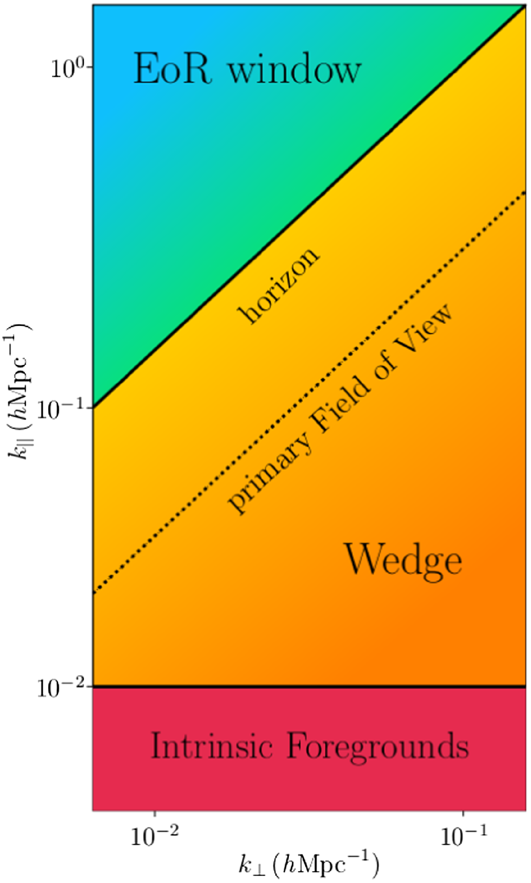
Figure 1. Schematic representation of the measured cylindrical power spectrum, based on Barry et al. (Reference Barry, Hazelton, Sullivan, Morales and Pober2016). The yellow region shows the wedge where the foregrounds are present. The blue region here shows the EoR window, free of foregrounds.
In the statistical detection of the 21 cm signal using the power spectrum, the traditional strategy is the wedge-avoidance method, where the search for the cosmological signal is restricted within the EoR window. As a result, the Fourier modes present within the wedge are unused even though the cosmological signal has higher strength in the lower
 $\mathrm{k}_{||}$
modes. However, if the 21 cm experiments can access the power in the lower
$\mathrm{k}_{||}$
modes. However, if the 21 cm experiments can access the power in the lower
 $\mathrm{k}_{||}$
modes, it can improve the possibility of a successful detection of the cosmological signal. The conceptually straightforward way to enlarge the EoR window is to subtract the foregrounds from the data directly. However, a perfect foreground model is necessary to accomplish this, which is not practical. On the contrary, the residual foregrounds can cause more problems to the power spectrum estimation than the foregrounds themselves (Trott, Wayth, & Tingay Reference Trott, Wayth and Tingay2012). Further, Liu, Parsons, & Trott (Reference Liu, Parsons and Trott2014) attempts to explore statistical methods by which the EoR window can be enlarged, thereby increasing the sensitivity of the power spectrum measurements. An alternative approach to enlarge the EoR window is to reduce the size of the wedge, as seen in the Fourier space. In the schematic representation, the ‘horizon’ line represents the expected contamination limits caused by sources in the sidelobes and the line representing the ‘primary field of view’ indicates the expected contamination limits resulting from sources within the primary Field of View (FoV) of the instrument. The best approach to reduce the size of the wedge is to use an instrument with a smaller FoV, which still retains the ability to measure the characteristic size scales of the cosmological signal, but removes unnecessary foregrounds. In this way, the ‘primary field of view’ line in the power spectrum will be reduced to lower
$\mathrm{k}_{||}$
modes, it can improve the possibility of a successful detection of the cosmological signal. The conceptually straightforward way to enlarge the EoR window is to subtract the foregrounds from the data directly. However, a perfect foreground model is necessary to accomplish this, which is not practical. On the contrary, the residual foregrounds can cause more problems to the power spectrum estimation than the foregrounds themselves (Trott, Wayth, & Tingay Reference Trott, Wayth and Tingay2012). Further, Liu, Parsons, & Trott (Reference Liu, Parsons and Trott2014) attempts to explore statistical methods by which the EoR window can be enlarged, thereby increasing the sensitivity of the power spectrum measurements. An alternative approach to enlarge the EoR window is to reduce the size of the wedge, as seen in the Fourier space. In the schematic representation, the ‘horizon’ line represents the expected contamination limits caused by sources in the sidelobes and the line representing the ‘primary field of view’ indicates the expected contamination limits resulting from sources within the primary Field of View (FoV) of the instrument. The best approach to reduce the size of the wedge is to use an instrument with a smaller FoV, which still retains the ability to measure the characteristic size scales of the cosmological signal, but removes unnecessary foregrounds. In this way, the ‘primary field of view’ line in the power spectrum will be reduced to lower
 $k_{||}$
modes enabling to access the k-modes within the wedge and thereby increasing the size of the EoR window to improve the probability of successful detection.
$k_{||}$
modes enabling to access the k-modes within the wedge and thereby increasing the size of the EoR window to improve the probability of successful detection.
To improve the probability of detecting the 21 cm signal for the Murchison Widefield Array (MWA, Tingay et al. Reference Tingay2013) telescope, we installed an external, zenith-pointing larger (
 $8\times8$
dipoles) antenna tile array called the Central Redundant Array Mega-tile (CRAM) as described in Paper I (Selvaraj et al. Reference Selvaraj, Wayth, Trott and Bhatia2024), and integrated it into the existing array configuration of the Phase II MWA (Wayth et al. Reference Wayth2018). The primary motivation for installing CRAM is that it is a larger tile array with a smaller FoV at every frequency under consideration compared to the regular MWA tile. The reduction in the FoV is equivalent to a narrower primary main lobe with multiple sidelobes. As a result, the ‘primary field of view’ line depicted in the schematic power spectrum (shown in Fig. 1) will be positioned towards the lower regions of the wedge, confining the foregrounds in accordance with the reduced primary beam of the instrument. However, the larger tile array achieves a smaller primary beam at the cost of a larger number of chromatic nulls which can potentially introduce additional errors. The chromaticity introduced due to the nulls in the antenna beam patterns can cause the foregrounds within the wedge to leak into the EoR window and contaminate the signal (Thyagarajan et al. Reference Thyagarajan2016). With the larger tile being twice the size of the MWA (which consists of
$8\times8$
dipoles) antenna tile array called the Central Redundant Array Mega-tile (CRAM) as described in Paper I (Selvaraj et al. Reference Selvaraj, Wayth, Trott and Bhatia2024), and integrated it into the existing array configuration of the Phase II MWA (Wayth et al. Reference Wayth2018). The primary motivation for installing CRAM is that it is a larger tile array with a smaller FoV at every frequency under consideration compared to the regular MWA tile. The reduction in the FoV is equivalent to a narrower primary main lobe with multiple sidelobes. As a result, the ‘primary field of view’ line depicted in the schematic power spectrum (shown in Fig. 1) will be positioned towards the lower regions of the wedge, confining the foregrounds in accordance with the reduced primary beam of the instrument. However, the larger tile array achieves a smaller primary beam at the cost of a larger number of chromatic nulls which can potentially introduce additional errors. The chromaticity introduced due to the nulls in the antenna beam patterns can cause the foregrounds within the wedge to leak into the EoR window and contaminate the signal (Thyagarajan et al. Reference Thyagarajan2016). With the larger tile being twice the size of the MWA (which consists of
 $4 \times 4$
dipoles) in each dimension and having equivalent spacing as the MWA, the nulls of the two beams align (see Figure 10 in Selvaraj et al. Reference Selvaraj, Wayth, Trott and Bhatia2024), minimising the effects of additional nulls. Additionally, in Selvaraj et al. (Reference Selvaraj, Wayth, Trott and Bhatia2024), it is shown that the CRAM has reduced sidelobe response when compared to MWA (see Figure 9a and 9b in Selvaraj et al. Reference Selvaraj, Wayth, Trott and Bhatia2024). Due to the lower response of the sidelobes, the corresponding power will be reduced near the horizon-EoR window boundary, limiting the leakage from the wedge to the EoR window. Thus, CRAM allows to access the k-modes near the horizon-EoR boundary, where the cosmological signal is stronger, thereby improving the probability of detection for MWA. The physical size of the larger tile is limited to the physical gap within the southern compact array of the Phase II configuration, where it is equidistant with the adjacent MWA tiles in an east-west orientation, forming redundant baselines with the regular MWA tiles. Even as the FoV of the instrument is reduced, it is still within the capability of measuring the characteristic size scale of the cosmological signal, where the proposed SKA beams have an even smaller FoV capable of detecting the ionised bubbles of reionisation (Mellema et al. Reference Mellema2013; Turner Reference Turner2015; Lin et al. Reference Lin, Oh, Furlanetto and Sutter2016; Braun et al. Reference Braun, Bonaldi, Bourke, Keane and Wagg2019). The instrument is currently active and was integrated with the MWA for the 2023 EoR observing season. Further details of the instrument are described in Paper I accompanied with this work (Selvaraj et al. Reference Selvaraj, Wayth, Trott and Bhatia2024).
$4 \times 4$
dipoles) in each dimension and having equivalent spacing as the MWA, the nulls of the two beams align (see Figure 10 in Selvaraj et al. Reference Selvaraj, Wayth, Trott and Bhatia2024), minimising the effects of additional nulls. Additionally, in Selvaraj et al. (Reference Selvaraj, Wayth, Trott and Bhatia2024), it is shown that the CRAM has reduced sidelobe response when compared to MWA (see Figure 9a and 9b in Selvaraj et al. Reference Selvaraj, Wayth, Trott and Bhatia2024). Due to the lower response of the sidelobes, the corresponding power will be reduced near the horizon-EoR window boundary, limiting the leakage from the wedge to the EoR window. Thus, CRAM allows to access the k-modes near the horizon-EoR boundary, where the cosmological signal is stronger, thereby improving the probability of detection for MWA. The physical size of the larger tile is limited to the physical gap within the southern compact array of the Phase II configuration, where it is equidistant with the adjacent MWA tiles in an east-west orientation, forming redundant baselines with the regular MWA tiles. Even as the FoV of the instrument is reduced, it is still within the capability of measuring the characteristic size scale of the cosmological signal, where the proposed SKA beams have an even smaller FoV capable of detecting the ionised bubbles of reionisation (Mellema et al. Reference Mellema2013; Turner Reference Turner2015; Lin et al. Reference Lin, Oh, Furlanetto and Sutter2016; Braun et al. Reference Braun, Bonaldi, Bourke, Keane and Wagg2019). The instrument is currently active and was integrated with the MWA for the 2023 EoR observing season. Further details of the instrument are described in Paper I accompanied with this work (Selvaraj et al. Reference Selvaraj, Wayth, Trott and Bhatia2024).
The primary objective of this work is to compare the performance of the new instrument CRAM with the regular MWA in the context of EoR science using power spectrum estimations via simulations of realistic sky models. To achieve this, we develop a power spectrum estimation pipeline for the hybrid setup consisting of two different baseline configurations. By analysing the 1D and 2D power spectra obtained from the MWA and CRAM baseline configurations, we aim to demonstrate that the CRAM baseline configuration offers better detection performance due to the reduced impact of foregrounds on the instrument with a reduced FoV, while preserving the 21 cm signal.
This paper begins with a detailed description of the mathematical framework for estimating the power spectrum in Section 2, followed by the development of the power spectrum pipeline for the hybrid setup in Section 3. The pipeline is validated with a point source sky model to confirm normalisation factors and verify power spectrum results, as presented in Section 4.1. We further test the pipeline using simulated diffuse sky maps and a simulated 21 cm signal to demonstrate its reliability in differentiating the signal’s spectral nature. The power spectrum results from foregrounds for both baseline configurations are presented in Section 4.2 and in Section 4.3, we present the 2D power spectrum results obtained using a simulated 21 cm signal. In Section 5, Fisher analysis is performed to quantitatively confirm the improvements made using CRAM compared to the regular MWA tiles. Finally, in Section 7, we conclude the work done in this paper. In this work, we perform all cosmological calculations based on Planck Collaboration et al. (2020), where
 $\mathrm{H_{0}} = 100\,{h}\,\mathrm{km}\,\mathrm{s}^{-1}\,\mathrm{Mpc}^{-1}$
.
$\mathrm{H_{0}} = 100\,{h}\,\mathrm{km}\,\mathrm{s}^{-1}\,\mathrm{Mpc}^{-1}$
.
2. Power spectrum: mathematical framework
The power spectrum in 21 cm experiments is a statistical tool used to quantify the statistical properties of the fluctuations in the 21 cm brightness temperature across the sky. In interferometry, the power spectrum is a natural product as the interferometer measures the Fourier Transform of the sky brightness distribution given by Thompson, Moran, & Swenson (Reference Thompson, Moran and Swenson2017)
 \begin{equation} \begin{aligned} V(u, v, w) &= \int_{-\infty}^{\infty} A_{N}(l, m)I(l, m) \times \exp \Bigg\{-j2\pi \Bigg[ul +vm + \\ &\quad w\Big( \sqrt{1 - l^2 - m^2}\Big) \Bigg] \Bigg\}\dfrac{dldm}{\Bigg( \sqrt{1 - l^2 - m^2}\Bigg)}, \end{aligned}\end{equation}
where
 $A_{N}(l, m)$
is the beam response of the instrument, I(l,m) is the sky brightness observed by the instrument and (l,m) is the directional cosine of the projection. The terms (u,v,w) are the coordinates of the physical positions of an antenna pair in the uv-plane given by
$A_{N}(l, m)$
is the beam response of the instrument, I(l,m) is the sky brightness observed by the instrument and (l,m) is the directional cosine of the projection. The terms (u,v,w) are the coordinates of the physical positions of an antenna pair in the uv-plane given by
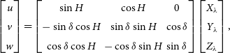 \begin{equation} \begin{bmatrix} u \\ v \\ w \end{bmatrix} = \begin{bmatrix} \sin H & \cos H & 0 \\ -\sin\delta\cos H & \sin\delta\sin H & \cos\delta\\ \cos\delta\cos H & -\cos\delta\sin H & \sin\delta \\ \end{bmatrix} \begin{bmatrix} X_{\lambda} \\ Y_{\lambda} \\ Z_{\lambda}\\ \end{bmatrix}, \end{equation}
where
 $(H, \delta)$
is the Hour Angle and declination of the phase centre of the observation; dependant upon the scanning strategy and
$(H, \delta)$
is the Hour Angle and declination of the phase centre of the observation; dependant upon the scanning strategy and
 $(X_{\lambda}, Y_{\lambda}, Z_{\lambda})$
is the global position of the antenna configuration under consideration in the units of wavelength. For a small FoV, where
$(X_{\lambda}, Y_{\lambda}, Z_{\lambda})$
is the global position of the antenna configuration under consideration in the units of wavelength. For a small FoV, where
 $|l| \ll 1$
and
$|l| \ll 1$
and
 $|m| \ll 1$
, w terms are negligible (Bond & Efstathiou Reference Bond and Efstathiou1987), and therefore the interferometer measurements are the two-dimensional Fourier Transform of the beam-attenuated sky distribution. The power spectrum as a function of spatial scale k (
$|m| \ll 1$
, w terms are negligible (Bond & Efstathiou Reference Bond and Efstathiou1987), and therefore the interferometer measurements are the two-dimensional Fourier Transform of the beam-attenuated sky distribution. The power spectrum as a function of spatial scale k (
 $\mathrm{hMpc}^{-1}$
) estimated from the complex visibility measurements made by the interferometer is given by
$\mathrm{hMpc}^{-1}$
) estimated from the complex visibility measurements made by the interferometer is given by
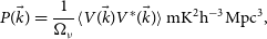 \begin{equation}P(\vec{k}) = \dfrac{1}{\Omega_\nu}\langle V(\vec{k})V^{*}(\vec{k})\rangle \, \mathrm{mK}^2\mathrm{h}^{-3}\mathrm{Mpc}^3,\end{equation}
where
 $V(\vec{k})$
is the visibility function and
$V(\vec{k})$
is the visibility function and
 $\Omega_\nu$
is the observing volume. In the k = (u,v,
$\Omega_\nu$
is the observing volume. In the k = (u,v,
 $\tau$
) space Fourier representation, the power spectrum is formed from visibilities in the dimensions of (u,v,
$\tau$
) space Fourier representation, the power spectrum is formed from visibilities in the dimensions of (u,v,
 $\tau$
), where the (u,v) is natively measured by the interferometer and
$\tau$
), where the (u,v) is natively measured by the interferometer and
 $\tau$
is generated by the Fourier Transform along the frequency axis.
$\tau$
is generated by the Fourier Transform along the frequency axis.
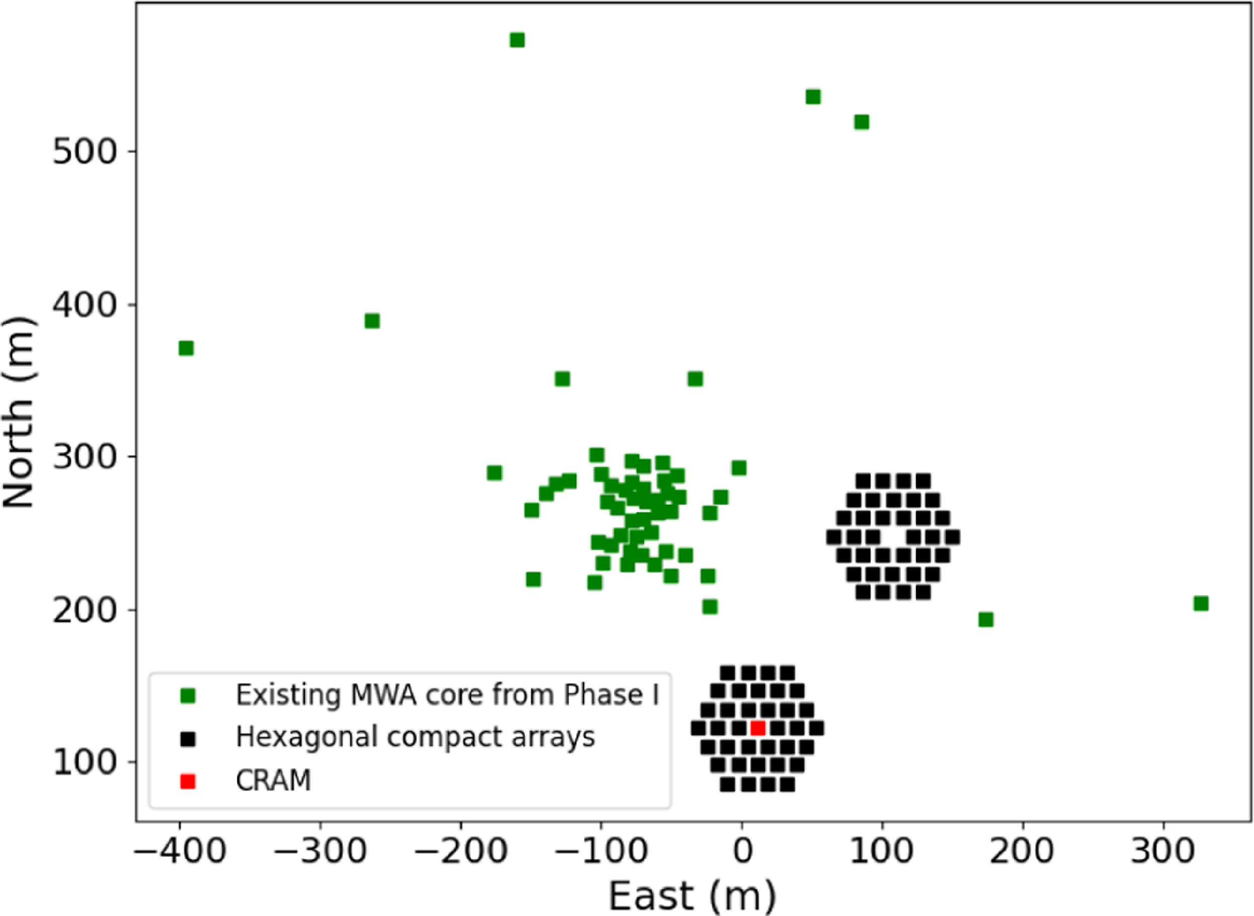
Figure 2. The Phase II MWA array configuration with the two hexagonal compact configurations shown in black markings placed alongside the original MWA Phase I tiles shown in green markings. The new instrument CRAM is located within the southern hexagonal compact array configuration and is shown in red marking.
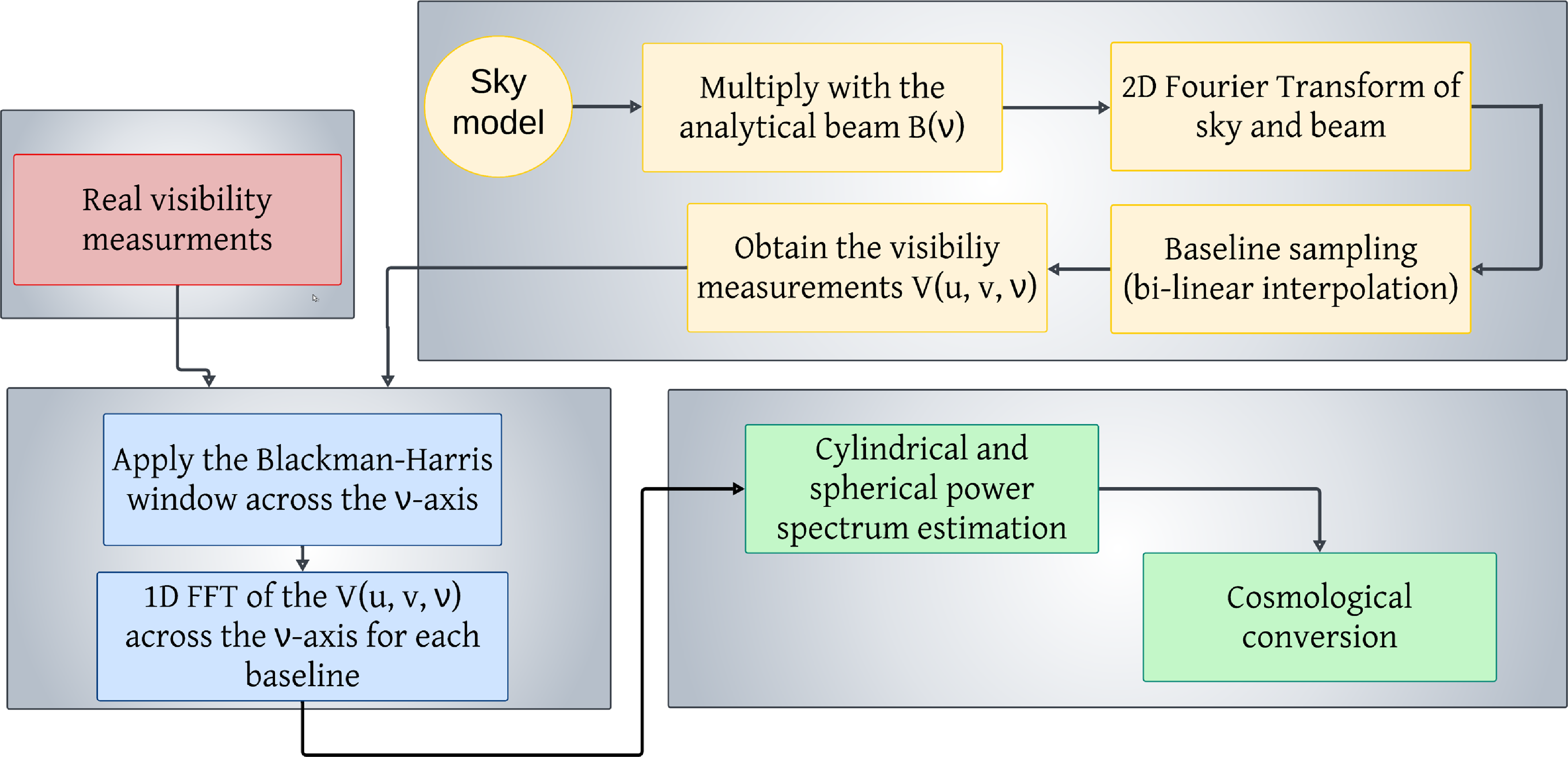
Figure 3. Block diagram representation of the hybrid power spectrum pipeline developed for this work. The pipeline is a combination of three separate steps: calculating the visibility measurement followed by computing the delay spectrum and then estimating the 2D and 1D power spectrum. Currently, the pipeline computes visibility using simulated sky models, but in the future, the simulated visibility measurements will be replaced with real visibility measurements obtained from the instrument.
3. Methodology
The primary motivation of this work is to utilise the new instrument CRAM, with a reduced FoV and sidelobe response compared to the regular MWA array, to suppress the smooth foregrounds while preserving the 21 cm signal. We aim to compare the detection signal-to-noise ratio (SNR) using power spectrum estimations and demonstrate that CRAM-MWA baselines are expected to have better detection performance. The comparison will be performed in both simulations and via Fisher analysis of the signal detectability. Using power spectrum estimations, we also aim to demonstrate that the reduction in the FoV does not affect the simulated 21 cm signal with spectral fluctuations. Hence, in this work, we built a pipeline to compute the power spectrum, similar to the work done in Nasirudin et al. (Reference Nasirudin2020), Cook, Trott, & Line (Reference Cook, Trott and Line2022), but for the hybrid setup consisting of two different antenna types: MWA and CRAM. For characterising the performance of the CRAM and the regular MWA tiles, we use the MWA Phase II compact array configuration that consists of two hexagonal compact arrays and the original core configuration from Phase I as shown in Fig. 2. For the first baseline setup consisting of MWA-MWA baselines, we utilise all the 128 antenna positions in the Phase II configuration, resulting in
 $8\,128$
baseline measurements. The second setup consists of utilising all the possible baselines made with the CRAM at the centre of the southern hexagon in the Phase II configuration, corresponding to 128 CRAM-MWA baseline measurements for each snapshot of observation.
$8\,128$
baseline measurements. The second setup consists of utilising all the possible baselines made with the CRAM at the centre of the southern hexagon in the Phase II configuration, corresponding to 128 CRAM-MWA baseline measurements for each snapshot of observation.
For the given array configuration, sky model and corresponding beam response of the instrument, using the pipeline, we simulate visibility measurements as a function of time in the frequency range of 165.75–185.75 MHz with a frequency resolution of 80 kHz to probe a redshift
 $z\in (7.5 - 6.64)$
. For the simulations, we adopt a zenith-pointed ‘drift and shift’ observation strategy using two-minute scans (Hour Angle
$z\in (7.5 - 6.64)$
. For the simulations, we adopt a zenith-pointed ‘drift and shift’ observation strategy using two-minute scans (Hour Angle
 $=\pm 1$
min), where the phase centre is defined as the LST (local sidereal time) in the middle of the scan. Each two-minute observation has a time resolution of eight seconds. Successive observations are separated by 10 min in these simulations. This strategy more closely resembles the HERA observation strategy because of the fixed zenith pointing and smaller FoV of the CRAM. The two-minute observations are sufficiently small that the sky remains relatively constant with respect to the beam, and the 10 min gap allows each snapshot to be independent. For illustration of the impact of foregrounds on the detectability of the cosmological signal, we simulate 24 hrs of data but note that actual EoR experiments have well-defined fields over a limited range of RA and try to avoid the impact of the Galactic plane.
$=\pm 1$
min), where the phase centre is defined as the LST (local sidereal time) in the middle of the scan. Each two-minute observation has a time resolution of eight seconds. Successive observations are separated by 10 min in these simulations. This strategy more closely resembles the HERA observation strategy because of the fixed zenith pointing and smaller FoV of the CRAM. The two-minute observations are sufficiently small that the sky remains relatively constant with respect to the beam, and the 10 min gap allows each snapshot to be independent. For illustration of the impact of foregrounds on the detectability of the cosmological signal, we simulate 24 hrs of data but note that actual EoR experiments have well-defined fields over a limited range of RA and try to avoid the impact of the Galactic plane.
Using the visibility measurements produced for each setup, the pipeline computes the delay spectrum by computing the Fourier Transform across frequency for each baseline and then averaging to produce 2D and 1D power spectrum. The complete schematic representation of the pipeline is shown in Fig. 3. The power spectrum pipeline built is tested and validated to confirm that it is reliable in differentiating the spectral nature of the signals. The section below elaborates on the method used to estimate the power spectrum using the pipeline for the hybrid setup.
3.1 Sky modelling
For the foreground simulations performed, we use the 159 MHz EDA2 all-sky map (Kriele et al. Reference Kriele, Wayth, Bentum, Juswardy and Trott2022), where it is scaled to the frequency range of 165.75–185.75 MHz with a spectral index map derived from EDA2 map and 408 MHz Haslam map. For a given frequency channel and pointing centre of the observation, we consider the corresponding two-dimensional orthogonal projection of the sky map (
 $I(l, m, \nu)$
) using HEALPix Python function orthview (Górski et al. Reference Górski2005). The sky map in the units of Kelvin is converted to Jy/pixel units using the standard Rayleigh-Jeans law. Thus, the 2D sky models are simulated for all pointing centres across the 24 hrs observing duration.
$I(l, m, \nu)$
) using HEALPix Python function orthview (Górski et al. Reference Górski2005). The sky map in the units of Kelvin is converted to Jy/pixel units using the standard Rayleigh-Jeans law. Thus, the 2D sky models are simulated for all pointing centres across the 24 hrs observing duration.
The one Jansky point source test, conducted for fewer pointing directions while the source remains within the primary beam, verifies the correctness and normalisation of the pipeline. For the 21 cm signal as the sky model, the power spectrum is estimated for a single pointing phase centre of observation. Further details of the 21 cm signal as sky model are included in Section 4.3.
3.2 Beam modelling
For each simulated two-minute observation, we utilise the zenith-pointing effective beam response of the baseline configuration to obtain the beam-weighted sky distribution image. The analytical beam models are produced for CRAM and MWA tiles as detailed in Section 3 of Paper I in the frequency range of 165.75–185.75 MHz. In the MWA-MWA baseline setup, the cross-correlation term (
 $A_{N}(l, m)$
) in the visibility Equation (1) is the cross-product of two regular MWA beams. On the contrary, in the second setup, the cross-correlation beam is the product of a regular MWA tile and the larger CRAM tile response. Section 3 of Paper I describes in detail the differences between the beam response patterns obtained for both instruments. Similar to the 2D sky image produced, we employ the orthogonal projection for each frequency channel to obtain the 2D image of the analytical beam model for the zenith pointing array. Thus, in our simulations for a given snapshot of observation, the sky remains the same for both the setup of baselines, while the effective beam response differs between the two baseline configurations.
$A_{N}(l, m)$
) in the visibility Equation (1) is the cross-product of two regular MWA beams. On the contrary, in the second setup, the cross-correlation beam is the product of a regular MWA tile and the larger CRAM tile response. Section 3 of Paper I describes in detail the differences between the beam response patterns obtained for both instruments. Similar to the 2D sky image produced, we employ the orthogonal projection for each frequency channel to obtain the 2D image of the analytical beam model for the zenith pointing array. Thus, in our simulations for a given snapshot of observation, the sky remains the same for both the setup of baselines, while the effective beam response differs between the two baseline configurations.
3.3 Simulating visibility measurements
To obtain the complex visibility measurements, the pipeline performs a Fourier Transform on the product of the sky brightness image and the beam response corresponding to the baseline setup for each sampling time within the two-minute observation of the drift scan, resulting in a 2D Fourier grid. This Fourier grid is sampled by interpolating between the regular discrete sample output by the transform using bi-linear interpolation for a known value of
 $\texttt{(u,v)}$
obtained from the baseline measurements as a function of frequency and sampling time to produce visibility measurements. Thus, for every frequency channel under consideration, visibility measurements are obtained for each baseline measurement at every
$\texttt{(u,v)}$
obtained from the baseline measurements as a function of frequency and sampling time to produce visibility measurements. Thus, for every frequency channel under consideration, visibility measurements are obtained for each baseline measurement at every
 $\texttt{(u,v)}$
sample within the two-minute snapshot of observation.
$\texttt{(u,v)}$
sample within the two-minute snapshot of observation.
3.4 Power spectrum estimation
This work employs the delay spectrum technique to estimate the power spectrum. The delay spectrum is computed by applying the Fourier Transform to the complex visibility measurement from each baseline across the frequency (Parsons et al. Reference Parsons, Pober, McQuinn, Jacobs and Aguirre2012a);
 \begin{equation} V_{b}(\tau) = \int V_{b}(\nu) e^{2\pi\nu\tau i} d\nu\,\mathrm{Jy}, \end{equation}
where
 $\tau$
is the delay and b is a given baseline. To reduce any spectral leakage caused by aliasing from the bandwidth-limited Fourier Transform in the frequency axis, a 4-term Blackman-Harris window is applied to the Fourier-transformed visibility measurements along the frequency axis. The delay transformed visibilities, after multiplying with the frequency resolution, is used to estimate the cosmological power spectrum given by
$\tau$
is the delay and b is a given baseline. To reduce any spectral leakage caused by aliasing from the bandwidth-limited Fourier Transform in the frequency axis, a 4-term Blackman-Harris window is applied to the Fourier-transformed visibility measurements along the frequency axis. The delay transformed visibilities, after multiplying with the frequency resolution, is used to estimate the cosmological power spectrum given by
 \begin{equation} P(k) = \tilde{V}(\vec{\tau}) \tilde{V}^{*}(\vec{\tau}) \,\mathrm{Jy}^{2}\mathrm{Hz}^{2}. \end{equation}
The cylindrical power spectrum is then mimicked by incoherently averaging the power in bins of the uv-plane after cosmological conversions given by
 \begin{equation}\begin{aligned}k_{\perp} &= \sqrt{k_{u}^2 + k_{v}^2}, \\k_{||} &= k_{\tau}.\end{aligned}\end{equation}
The conversion from observations to cosmological dimension (
 $\mathrm{mK}^2\mathrm{h}^{-3}\mathrm{Mpc}^3$
) are described in Morales & Hewitt (Reference Morales and Hewitt2004) and will vary for both the setup of instruments under consideration in this work.
$\mathrm{mK}^2\mathrm{h}^{-3}\mathrm{Mpc}^3$
) are described in Morales & Hewitt (Reference Morales and Hewitt2004) and will vary for both the setup of instruments under consideration in this work.
Overall, the power spectrum estimated in this work results from three separate procedures described in this section (illustrated as three separate sections in Fig. 3). In this work, we utilise only simulated sky models and analytical beam models to estimate the power spectrum, demonstrating the improvement achievable with an instrument that has a reduced FoV. In the future, the simulated visibility measurements used in the first block of the pipeline (shown in yellow in Fig. 3) will be replaced with real visibility measurements (as shown in red in Fig. 3) obtained with the instrument to estimate the power spectrum.
4. Results
The pipeline’s performance is validated using 1 Jansky point source, diffuse foregrounds, and a simulated 21 cm signal. The 1 Jansky point source test verifies the normalisation used in the pipeline, while foreground simulations demonstrate the CRAM’s ability to suppress foregrounds, and 21 cm simulations showcase the pipeline’s robustness in measuring cosmological power. Results from each of these tests are presented in the following section.
4.1 Point source sky model
The proof of concept developed in this work is validated using a 1 Jansky point source to verify the normalisation used in the pipeline. The pipeline computes the 2D and 1D power spectra for a two-minute snapshot of observation when the phase centre is at the zenith. Fig. 4 shows the resultant cylindrical power spectrum obtained when the point source is at the beam centre of the two instruments, demonstrating equal power in the DC mode regardless of baseline configuration. This is confirmed by the power in the DC mode of the 2D power spectrum, which matches the estimated analytical solution of
 $\sim 10^{11}\,\mathrm{mK}^2\mathrm{h}^{-3}\mathrm{Mpc}^3$
, as shown in Fig. 4. We further validate the pipeline with observations at different phase centre pointings, such that the point source transits through the primary beam of the instrument, revealing instances where the wedge demonstrated consistent power across both configurations, with differences evident only at the edge of the wedge. It is noteworthy to point out here that we are particularly interested in snapshots of observations, where the power at the edge of the wedge varies for the two baseline configurations. However, a point source sky model is trivial in further validating the performance of the pipeline.
$\sim 10^{11}\,\mathrm{mK}^2\mathrm{h}^{-3}\mathrm{Mpc}^3$
, as shown in Fig. 4. We further validate the pipeline with observations at different phase centre pointings, such that the point source transits through the primary beam of the instrument, revealing instances where the wedge demonstrated consistent power across both configurations, with differences evident only at the edge of the wedge. It is noteworthy to point out here that we are particularly interested in snapshots of observations, where the power at the edge of the wedge varies for the two baseline configurations. However, a point source sky model is trivial in further validating the performance of the pipeline.
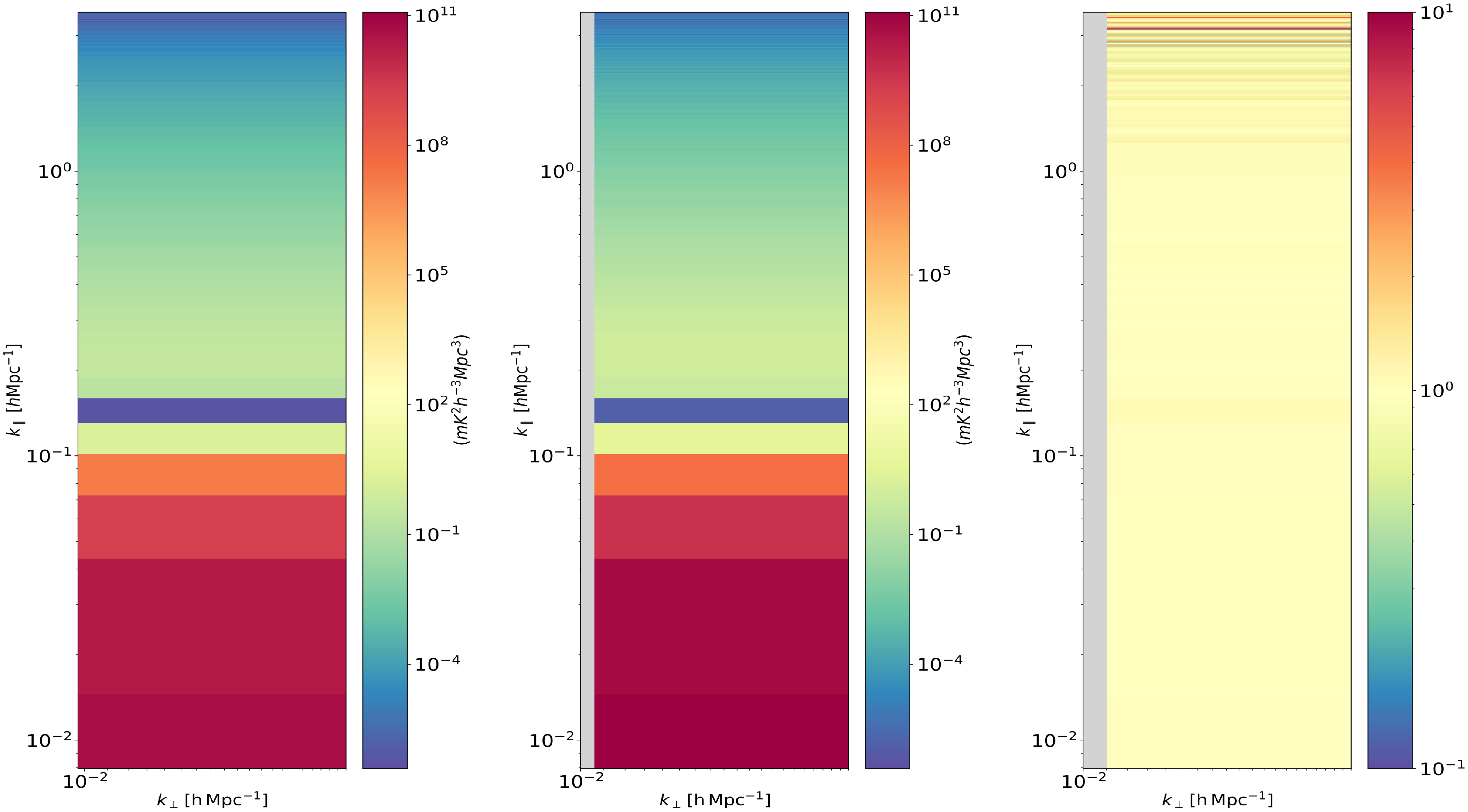
Figure 4. The cylindrically-averaged 2D power spectrum obtained with 1 Jansky point source, where the phase centre is at the zenith and hence the point source is at the beam centre for both the instruments. The left panel shows the power spectrum obtained using the MWA-MWA baselines, the middle panel shows the power spectrum obtained using the CRAM-MWA baselines, and the third panel shows the ratio of the power spectrum obtained from the CRAM-MWA baselines to that obtained from the MWA-MWA baselines. All the three plots have
 $k_{\perp}$
in the x-axis and
$k_{\perp}$
in the x-axis and
 $k_{||}$
in the y-axis in log-scale in the units of
$k_{||}$
in the y-axis in log-scale in the units of
 $h\mathrm{Mpc}^{-1}$
. The power spectrum thus obtained shows equal DC mode value corresponding to the analytical solution of
$h\mathrm{Mpc}^{-1}$
. The power spectrum thus obtained shows equal DC mode value corresponding to the analytical solution of
 $\sim 10^{11}\,m\mathrm{K}^{2}\mathrm{h}^{-3}\mathrm{Mpc}^3$
for the two baseline configurations.
$\sim 10^{11}\,m\mathrm{K}^{2}\mathrm{h}^{-3}\mathrm{Mpc}^3$
for the two baseline configurations.
4.2 Diffuse foregrounds
The pipeline is further tested using the EDA2 diffuse sky map. The 2D and 1D power spectrum are estimated for every two-minute snapshot across the 24 hrs of simulation. Fig. 5 shows the cylindrically-averaged power spectrum obtained for a snapshot of observation when the phase centre is at
 $\mathrm{RA} = 12$
hrs 2 min (observation snapshot randomly selected), with MWA-MWA and CRAM-MWA baseline configurations. The power spectrum obtained using the MWA-MWA baselines has a power of the order
$\mathrm{RA} = 12$
hrs 2 min (observation snapshot randomly selected), with MWA-MWA and CRAM-MWA baseline configurations. The power spectrum obtained using the MWA-MWA baselines has a power of the order
 $\sim$
 $10^{14}\,\mathrm{mK}^2\mathrm{h}^{-3}\mathrm{Mpc}^3$
in the lower
$10^{14}\,\mathrm{mK}^2\mathrm{h}^{-3}\mathrm{Mpc}^3$
in the lower
 $k_{||}$
modes. In comparison, the power spectrum from CRAM-MWA baselines has a power of the order
$k_{||}$
modes. In comparison, the power spectrum from CRAM-MWA baselines has a power of the order
 $\sim$
 $10^{12}\,\mathrm{mK}^2\mathrm{h}^{-3}\mathrm{Mpc}^3$
. Fig. 6 shows the corresponding sky model obtained for the phase centre pointing at
$10^{12}\,\mathrm{mK}^2\mathrm{h}^{-3}\mathrm{Mpc}^3$
. Fig. 6 shows the corresponding sky model obtained for the phase centre pointing at
 $\mathrm{RA} = 12$
hrs 2 min as seen by the MWA and CRAM beams. The sky model confirms the presence of the Galactic plane in the sidelobes of both beams; however, the reduced sidelobe response from CRAM results in lower power compared to the MWA response. The sky response of MWA has Centaurus A in its primary beam, while it is present in a sidelobe for the CRAM baseline. Hence, the two orders of magnitude reduction in power observed with CRAM-MWA baselines is attributed to the pointing centre, where the bright foregrounds present in the MWA-MWA baselines are attenuated in the CRAM-MWA baselines, consistent with the reduced FoV and sidelobe response of CRAM. A corresponding reduction in power is observed in the higher
$\mathrm{RA} = 12$
hrs 2 min as seen by the MWA and CRAM beams. The sky model confirms the presence of the Galactic plane in the sidelobes of both beams; however, the reduced sidelobe response from CRAM results in lower power compared to the MWA response. The sky response of MWA has Centaurus A in its primary beam, while it is present in a sidelobe for the CRAM baseline. Hence, the two orders of magnitude reduction in power observed with CRAM-MWA baselines is attributed to the pointing centre, where the bright foregrounds present in the MWA-MWA baselines are attenuated in the CRAM-MWA baselines, consistent with the reduced FoV and sidelobe response of CRAM. A corresponding reduction in power is observed in the higher
 $k_{||}$
modes towards the EoR window as shown in the ratio of the power spectrum in the third panel of Fig. 5. The blue colour scale in the ratio plot, which represents values less than one, indicates that with CRAM, a larger array tile with a smaller FoV, the foregrounds have a lesser impact when compared to the regular MWA. Specifically, note that at
$k_{||}$
modes towards the EoR window as shown in the ratio of the power spectrum in the third panel of Fig. 5. The blue colour scale in the ratio plot, which represents values less than one, indicates that with CRAM, a larger array tile with a smaller FoV, the foregrounds have a lesser impact when compared to the regular MWA. Specifically, note that at
 $k_{||}\sim0.01\,\mathrm{hMpc}^{-1}$
the power spectrum obtained with CRAM-MWA baseline has power less than the power obtained using MWA-MWA baseline. However, the ratio plot shown depends upon the observation phase centre that decides how the sky is aligned within the primary beam under consideration. Thus, as expected for an instrument with a smaller FoV, such as CRAM, can suppress the smooth foreground signal and access the k-modes present towards the lower
$k_{||}\sim0.01\,\mathrm{hMpc}^{-1}$
the power spectrum obtained with CRAM-MWA baseline has power less than the power obtained using MWA-MWA baseline. However, the ratio plot shown depends upon the observation phase centre that decides how the sky is aligned within the primary beam under consideration. Thus, as expected for an instrument with a smaller FoV, such as CRAM, can suppress the smooth foreground signal and access the k-modes present towards the lower
 $k_{||}$
modes near the horizon-EoR window boundary, where the cosmological signal has higher strength.
$k_{||}$
modes near the horizon-EoR window boundary, where the cosmological signal has higher strength.
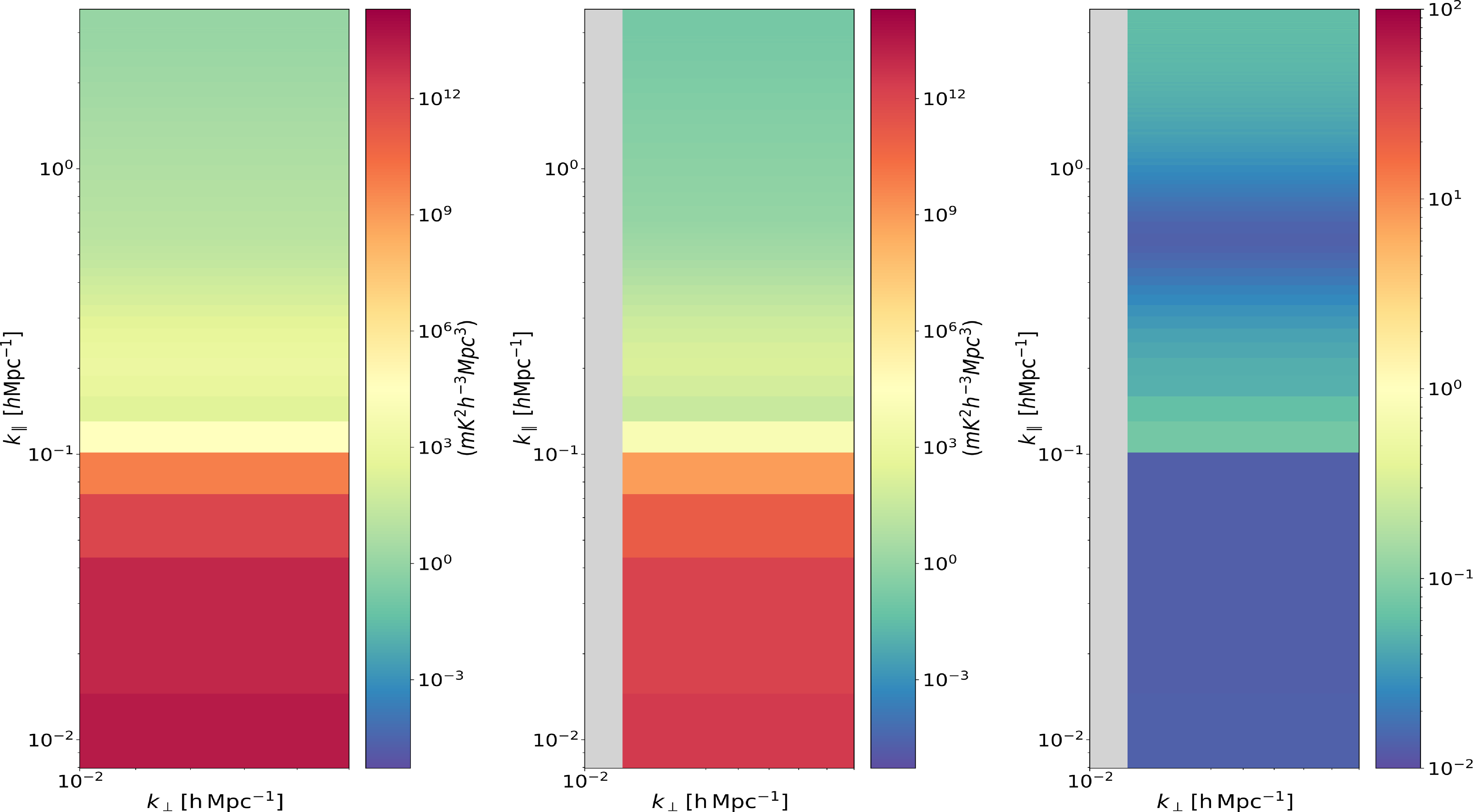
Figure 5. The cylindrically-averaged 2D power spectrum obtained with a diffuse sky model, measured at phase centre
 $\mathrm{RA} = 12$
hrs 2 min. The left panel shows the power spectrum obtained using MWA-MWA baselines, the middle panel shows the power spectrum obtained using CRAM-MWA baselines, and the third panel shows the ratio of the power spectrum obtained from the CRAM-MWA baseline to that obtained from the MWA-MWA baselines. All the three plots have
$\mathrm{RA} = 12$
hrs 2 min. The left panel shows the power spectrum obtained using MWA-MWA baselines, the middle panel shows the power spectrum obtained using CRAM-MWA baselines, and the third panel shows the ratio of the power spectrum obtained from the CRAM-MWA baseline to that obtained from the MWA-MWA baselines. All the three plots have
 $k_{\perp}$
in the x-axis and
$k_{\perp}$
in the x-axis and
 $k_{||}$
in the y-axis in log-scale in the units of
$k_{||}$
in the y-axis in log-scale in the units of
 $\mathrm{h}\mathrm{Mpc}^{-1}$
. In comparison to the power spectrum obtained from MWA-MWA baselines, the power spectrum obtained with CRAM baseline demonstrates two orders of magnitude reduction in the power, due to the differences in the apparent sky, as shown in Fig. 6.
$\mathrm{h}\mathrm{Mpc}^{-1}$
. In comparison to the power spectrum obtained from MWA-MWA baselines, the power spectrum obtained with CRAM baseline demonstrates two orders of magnitude reduction in the power, due to the differences in the apparent sky, as shown in Fig. 6.
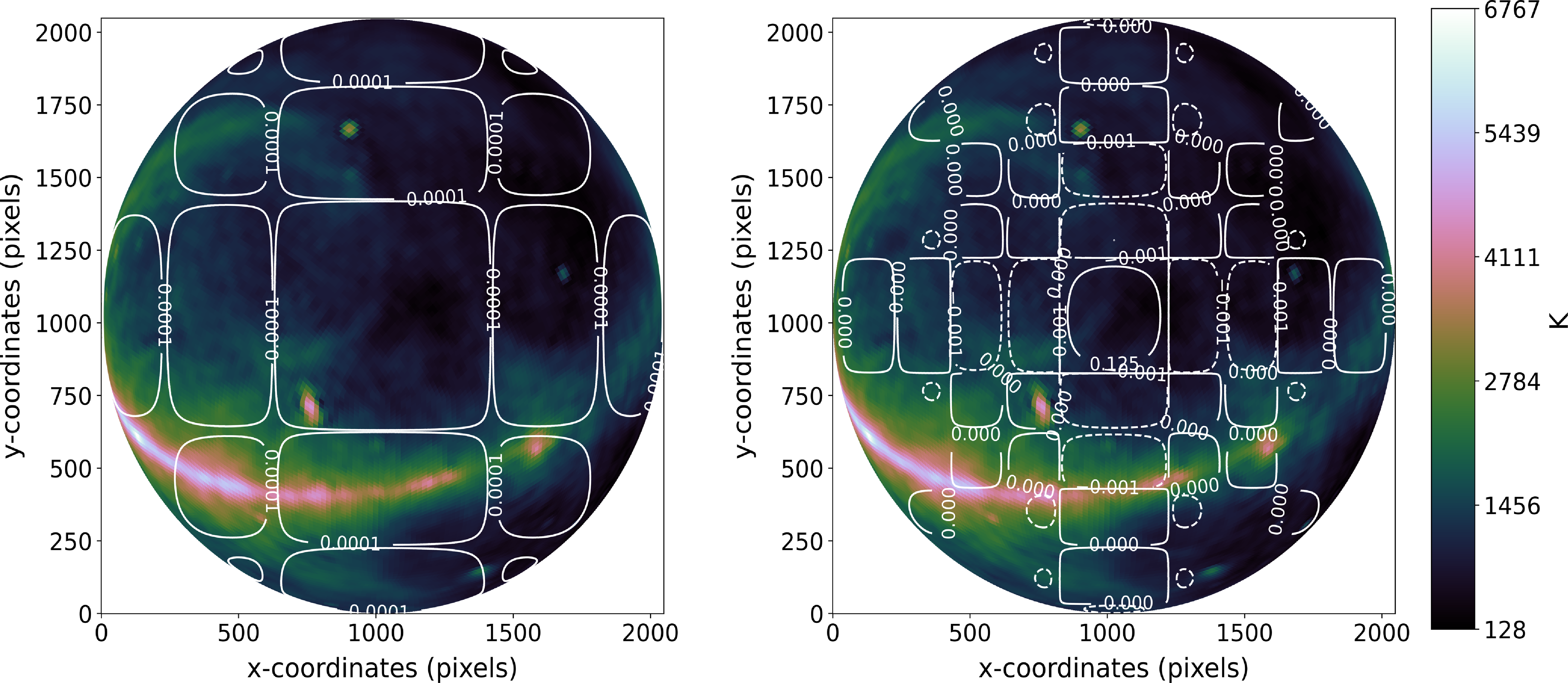
Figure 6. The sky response obtained at the phase centre,
 $\mathrm{RA} = 12$
hrs 2 min, is shown in the left panel for the MWA telescope and in the right panel for CRAM (over-plotted with the beam contour plot). Both beams have the Galactic Plane in their sidelobes; however, the corresponding power obtained with CRAM will be smaller due to its reduced sidelobe response compared to MWA. The sky model also shows the presence of Centaurus A within the primary beam of MWA, while it is within the sidelobes of the CRAM beam, leading to a reduced response for the CRAM configuration.
$\mathrm{RA} = 12$
hrs 2 min, is shown in the left panel for the MWA telescope and in the right panel for CRAM (over-plotted with the beam contour plot). Both beams have the Galactic Plane in their sidelobes; however, the corresponding power obtained with CRAM will be smaller due to its reduced sidelobe response compared to MWA. The sky model also shows the presence of Centaurus A within the primary beam of MWA, while it is within the sidelobes of the CRAM beam, leading to a reduced response for the CRAM configuration.
As observed in other power spectrum results obtained using Phase II configuration, this work also reports the presence of a vertical structure of high power towards larger
 $k_{\bot}$
modes associated with the missing baseline lengths and the physical gap between the compact array and the central core of Phase II MWA configuration (i.e. the weights are small here). These missing baselines were masked in our analysis and depicted in grey. The longest baseline obtained with CRAM is 482 m corresponding to
$k_{\bot}$
modes associated with the missing baseline lengths and the physical gap between the compact array and the central core of Phase II MWA configuration (i.e. the weights are small here). These missing baselines were masked in our analysis and depicted in grey. The longest baseline obtained with CRAM is 482 m corresponding to
 $k_{\perp}\sim0.3 \,\,\mathrm{hMpc}^{-1}$
. As a result, the characteristic wedge is not evident in the cylindrical power spectrum. In the power spectrum results, we have placed upper limits to the value of
$k_{\perp}\sim0.3 \,\,\mathrm{hMpc}^{-1}$
. As a result, the characteristic wedge is not evident in the cylindrical power spectrum. In the power spectrum results, we have placed upper limits to the value of
 $k_{\perp}$
modes not to be greater than
$k_{\perp}$
modes not to be greater than
 $0.02\,\,\mathrm{hMpc}^{-1}$
to avoid the missing baselines.
$0.02\,\,\mathrm{hMpc}^{-1}$
to avoid the missing baselines.
To further demonstrate the performance of CRAM, we present the 1D power spectrum in Fig. 7 obtained for a phase centre,
 $\mathrm{RA} = 0$
hrs 41 min. The resultant shape of the 1D power spectrum is expected from the instruments of different specifications. However, for this phase centre where the sky is relatively empty, the CRAM configuration does not produce a factor of two reduction in power. This confirms that the power reduction varies for different snapshots of the sky. Nonetheless, there is a consistent trend across the 24 hrs of observation, showing a lower response with the CRAM-MWA baseline compared to the MWA-MWA baseline and is quantitatively confirmed with the Fisher analysis conducted in Section 5.
$\mathrm{RA} = 0$
hrs 41 min. The resultant shape of the 1D power spectrum is expected from the instruments of different specifications. However, for this phase centre where the sky is relatively empty, the CRAM configuration does not produce a factor of two reduction in power. This confirms that the power reduction varies for different snapshots of the sky. Nonetheless, there is a consistent trend across the 24 hrs of observation, showing a lower response with the CRAM-MWA baseline compared to the MWA-MWA baseline and is quantitatively confirmed with the Fisher analysis conducted in Section 5.
4.3 21 cm signal
The power spectrum results obtained in this work demonstrate that the impact of foregrounds can be reduced by incorporating an instrument with a reduced FoV such as the CRAM. This reduction in foreground power is possible due to the smooth spectral nature of the signal, where the power from foregrounds is concentrated towards the lower k
 $_{||}$
modes of the 2D power spectrum (as shown in Fig. 1). On the contrary, the isotropic 21 cm signal is symmetric in Fourier space, and its spectral structure reflects true sky signal. Therefore, an instrument with a FoV capable of measuring the characteristic size scale of the cosmological signal should retain the power at all k-modes for the 21 cm cosmological signal.
$_{||}$
modes of the 2D power spectrum (as shown in Fig. 1). On the contrary, the isotropic 21 cm signal is symmetric in Fourier space, and its spectral structure reflects true sky signal. Therefore, an instrument with a FoV capable of measuring the characteristic size scale of the cosmological signal should retain the power at all k-modes for the 21 cm cosmological signal.
Further in this work, we demonstrate that the two pipelines developed with the hybrid setup can measure equivalent power spectrum outputs for a simulated 21 cm signal. For demonstration, we utilise large-volume simulations of the 21 cm signal produced by Greig et al. (Reference Greig, Wyithe, Murray, Mutch and Trott2022), a modified version of the semi-numerical 21CMFAST curated specifically for MWA. The 21 cm simulations correspond to the frequency band of 167–197 MHz (
 $z \sim 7.5-6.2$
) with
$z \sim 7.5-6.2$
) with
 $\sim$
80 kHz frequency resolution and comoving transverse side length
$\sim$
80 kHz frequency resolution and comoving transverse side length
 $7.5$
Gpc of
$7.5$
Gpc of
 $6400$
voxels. However, in this work, we only utilise a subset of the 21 cm box, corresponding to 2048 voxels in the frequency band of 167.75–185.75 MHz to save computational time. Fig. 8 shows the resultant 21 cm power spectrum obtained with the two pipelines developed. Both pipelines produce power outputs of
$6400$
voxels. However, in this work, we only utilise a subset of the 21 cm box, corresponding to 2048 voxels in the frequency band of 167.75–185.75 MHz to save computational time. Fig. 8 shows the resultant 21 cm power spectrum obtained with the two pipelines developed. Both pipelines produce power outputs of
 $\sim$
 $10^5\,\mathrm{mK}^2\mathrm{h}^{-3}\mathrm{Mpc}^3$
, as expected for the simulated 21 cm signal at redshift
$10^5\,\mathrm{mK}^2\mathrm{h}^{-3}\mathrm{Mpc}^3$
, as expected for the simulated 21 cm signal at redshift
 $z \sim 7.08$
. The comparable power levels obtained with the two different instruments, despite their differing FoV, demonstrate that both pipelines effectively capture the power of an unsmooth signal like the 21 cm signal. This confirms that the pipeline developed with the hybrid instrument setup can retain the cosmological signal while the impact of the foregrounds is reduced in accordance with the FoV of the instrument.
$z \sim 7.08$
. The comparable power levels obtained with the two different instruments, despite their differing FoV, demonstrate that both pipelines effectively capture the power of an unsmooth signal like the 21 cm signal. This confirms that the pipeline developed with the hybrid instrument setup can retain the cosmological signal while the impact of the foregrounds is reduced in accordance with the FoV of the instrument.
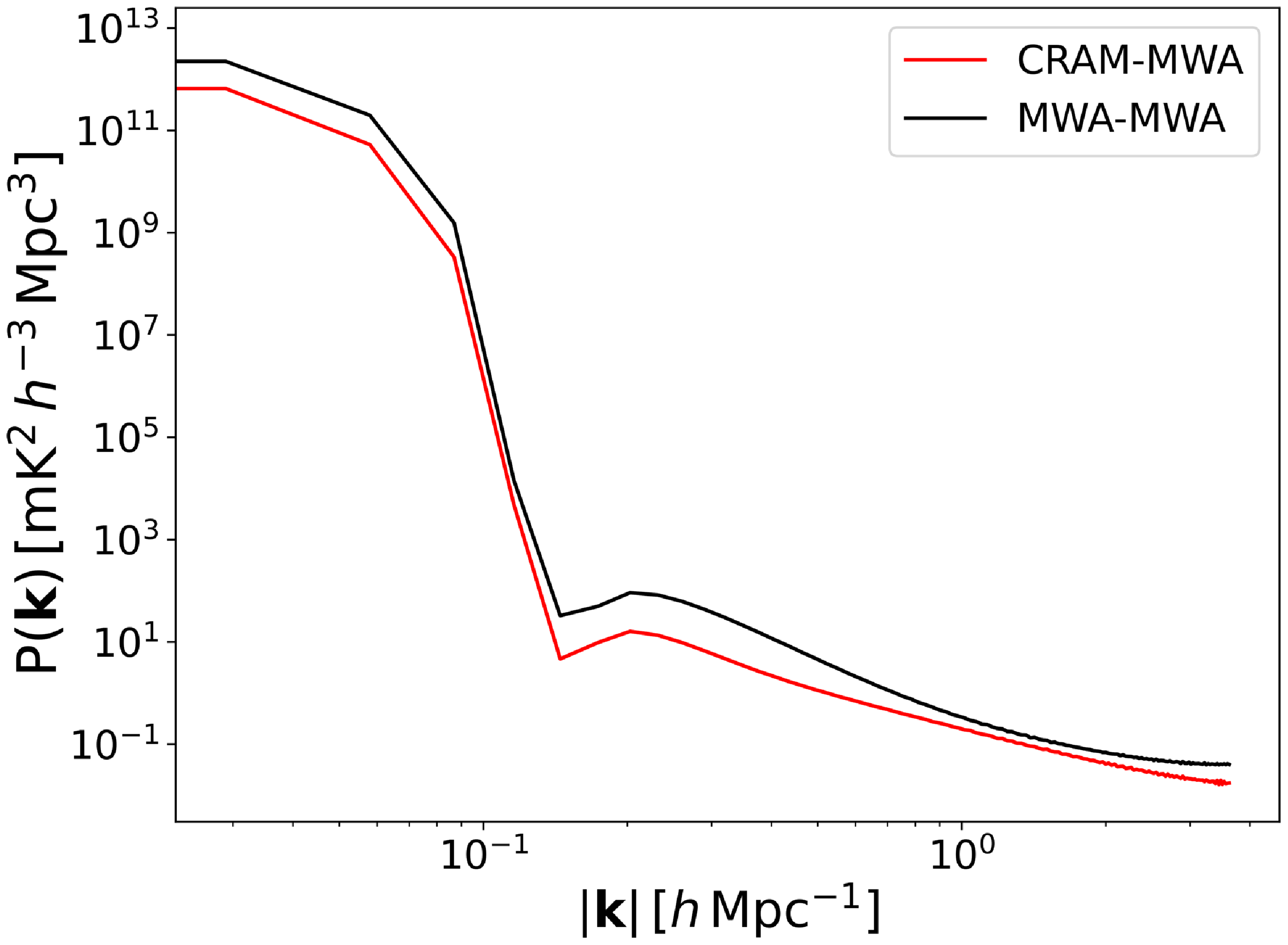
Figure 7. The 1D power spectrum obtained with a diffuse sky model corresponding to the phase centre,
 $\mathrm{RA} = 0$
hrs 41 min, where the sky is relatively empty. For this phase centre, the CRAM configuration shows a smaller reduction in power, confirming that the power reduction varies for different pointing centres of observation.
$\mathrm{RA} = 0$
hrs 41 min, where the sky is relatively empty. For this phase centre, the CRAM configuration shows a smaller reduction in power, confirming that the power reduction varies for different pointing centres of observation.
5. Fisher analysis
The power spectrum results demonstrate that the CRAM-MWA baselines have a reduced response for foregrounds compared to the MWA-MWA baselines, as expected, at the edge of the wedge. We will estimate the precision on the amplitude and slope of the power spectrum as our two parameters in the presence of unmodelled foregrounds, which we treat as the noise in our data. For a given parameter
 $\theta$
that we intend to estimate, the likelihood of the given data x is given as
$\theta$
that we intend to estimate, the likelihood of the given data x is given as
 $L(x;\; \theta$
). The Fisher matrix, which measures the information content for a given setup, is given by (Fisher Reference Fisher1935),
$L(x;\; \theta$
). The Fisher matrix, which measures the information content for a given setup, is given by (Fisher Reference Fisher1935),
 \begin{equation} F_{\alpha, \beta} = - \left\langle \frac{\partial^2 \mathrm{ln} L}{\partial \theta_{\alpha} \partial\theta_{\beta}} \right\rangle, \\ \end{equation}
where
 $(\alpha, \beta)$
are the two parameters under consideration. Using the Cramer-Rao theorem, the covariance matrix of the parameters is given by the inverse of the Fisher matrix. The variance on the parameters is given by the diagonal of the covariance matrix.
$(\alpha, \beta)$
are the two parameters under consideration. Using the Cramer-Rao theorem, the covariance matrix of the parameters is given by the inverse of the Fisher matrix. The variance on the parameters is given by the diagonal of the covariance matrix.
For this work, we use the 21 cm power spectrum model created by Mesinger, Furlanetto, & Cen (Reference Mesinger, Furlanetto and Cen2011) using the software simulation package 21CMFAST, a semi-numeric modelling tool designed to simulate the cosmological signal. We utilise the 21 cm 1D power spectrum at a redshift of
 $z \sim 7.08$
corresponding to the central frequency of
$z \sim 7.08$
corresponding to the central frequency of
 $175.75$
MHz used in the simulations. The fiducial 21 cm power spectrum in the units of (
$175.75$
MHz used in the simulations. The fiducial 21 cm power spectrum in the units of (
 $\mathrm{mK}^{2}$
) is converted to the cosmological units using
$\mathrm{mK}^{2}$
) is converted to the cosmological units using
 \begin{align} P_{21}^{2}(k) &= \dfrac{2\pi^{2}}{k^{3}}\Delta^{2}(k)\,\mathrm{mK}^2\mathrm{h}^{-3}\mathrm{Mpc}^3, \end{align}
where
 $\Delta^{2}(k)$
is the 21 cm power spectrum calculated using 21CMFAST, and
$\Delta^{2}(k)$
is the 21 cm power spectrum calculated using 21CMFAST, and
 \begin{equation}\log_{10}P_{21}(k) = m\log_{10}k + C,\end{equation}
where m is the slope and C is the normalisation constant when k = 1. The 21 cm power spectrum obtained is fitted with a straight line as shown in Fig. 9 to calculate the Fisher matrix using Equation (7). The straight line in log-scale given by Equation (9) is differentiated with respect to the slope and normalisation constant to obtain the covariance matrix. A complete description of the Fisher matrix derivation is detailed in Appendix A.
The CRAM-MWA baseline configuration allows to access extra k-modes of the 21 cm signal as shown in Fig. 10 when compared to the MWA-MWA baseline as it has a lower response to the foreground noise. The estimation of the covariance matrix allows us to evaluate the k-modes that can be accessed by using the power spectrum estimations. Considering the signal to be the fiducial 21 cm signal and noise to be the foreground estimation from the power spectrum, the SNR is calculated using
 \begin{equation} SNR = \dfrac{m}{\sqrt{\Sigma_{11}}},\end{equation}
where m is the slope of the straight line used to fit the 21 cm signal and
 $\Sigma_{11}$
is the first element in the covariance matrix obtained for a given power spectrum estimation. The resultant SNR estimation on the slope, obtained for different snapshots across LSTs is shown in Fig. 11. Over the 24 hrs of observation, the CRAM baselines report higher SNR when compared with the MWA baseline as expected from the foreground power levels measured by the two baseline configurations. During LST
$\Sigma_{11}$
is the first element in the covariance matrix obtained for a given power spectrum estimation. The resultant SNR estimation on the slope, obtained for different snapshots across LSTs is shown in Fig. 11. Over the 24 hrs of observation, the CRAM baselines report higher SNR when compared with the MWA baseline as expected from the foreground power levels measured by the two baseline configurations. During LST
 $\sim$
0-10 hrs, where the sky is relatively empty, both baseline configurations exhibit high SNR measurements. However, at LST
$\sim$
0-10 hrs, where the sky is relatively empty, both baseline configurations exhibit high SNR measurements. However, at LST
 $\sim$
18 hrs, the Galactic centre transits through the primary beam of both instruments, resulting in high foreground power for both the power spectrum results. Therefore, the SNR measurement is lower for both the baseline configurations than the previous snapshots of observations. Additionally, it can be noted that the SNR results obtained with CRAM baselines have more variations when compared to the results obtained using MWA baselines. The reason for these fluctuations is due to the larger number of nulls present for the larger antenna tile CRAM (refer to Figure 9a and 9b in Paper I) as the sky transits through them. However, across the 24 hrs of observation, it can be confirmed that the foregrounds have a lesser impact on power spectrum results obtained using the hybrid setup of CRAM-MWA baselines.
$\sim$
18 hrs, the Galactic centre transits through the primary beam of both instruments, resulting in high foreground power for both the power spectrum results. Therefore, the SNR measurement is lower for both the baseline configurations than the previous snapshots of observations. Additionally, it can be noted that the SNR results obtained with CRAM baselines have more variations when compared to the results obtained using MWA baselines. The reason for these fluctuations is due to the larger number of nulls present for the larger antenna tile CRAM (refer to Figure 9a and 9b in Paper I) as the sky transits through them. However, across the 24 hrs of observation, it can be confirmed that the foregrounds have a lesser impact on power spectrum results obtained using the hybrid setup of CRAM-MWA baselines.
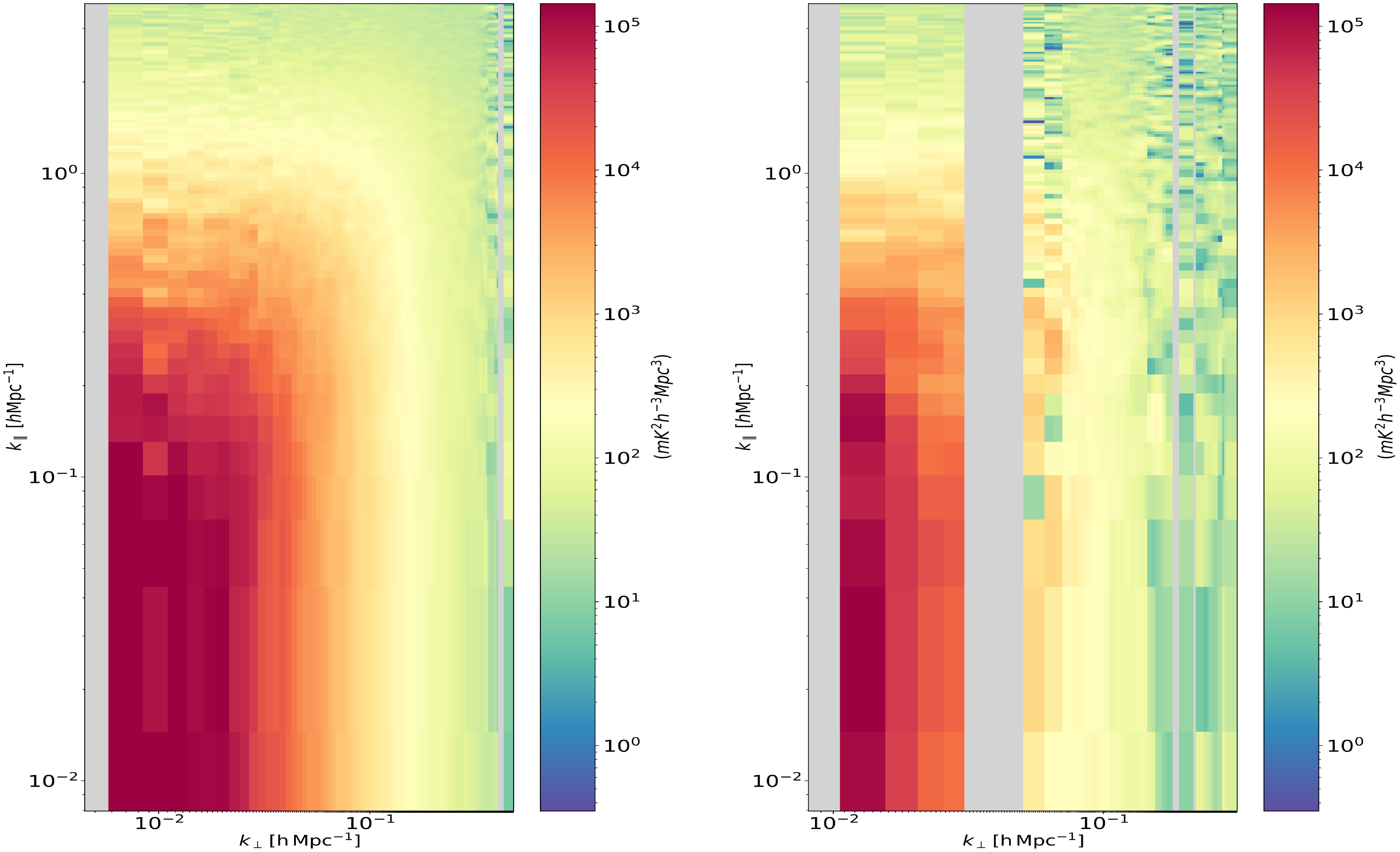
Figure 8. The 2D power spectrum obtained for the simulated 21cm signal using the two pipelines developed. The left panel shows the power spectrum obtained using MWA-MWA baselines and the right panel shows the power spectrum obtained using the CRAM-MWA baselines. Both the plots have
 $k_{\perp}$
in the x-axis and
$k_{\perp}$
in the x-axis and
 $k_{||}$
in the y-axis in log-scale in the units of
$k_{||}$
in the y-axis in log-scale in the units of
 $h\mathrm{Mpc}^{-1}$
. The two pipelines consisting of instruments with different FoV produce equivalent power levels of
$h\mathrm{Mpc}^{-1}$
. The two pipelines consisting of instruments with different FoV produce equivalent power levels of
 $\sim 10^5\,\mathrm{mK}^2\mathrm{h}^{-3}\mathrm{Mpc}^3$
as expected for the simulated 21 cm signal at redshift
$\sim 10^5\,\mathrm{mK}^2\mathrm{h}^{-3}\mathrm{Mpc}^3$
as expected for the simulated 21 cm signal at redshift
 $z \sim 7.08$
. For either setup, there are missing baselines that are greyed out in the results.
$z \sim 7.08$
. For either setup, there are missing baselines that are greyed out in the results.
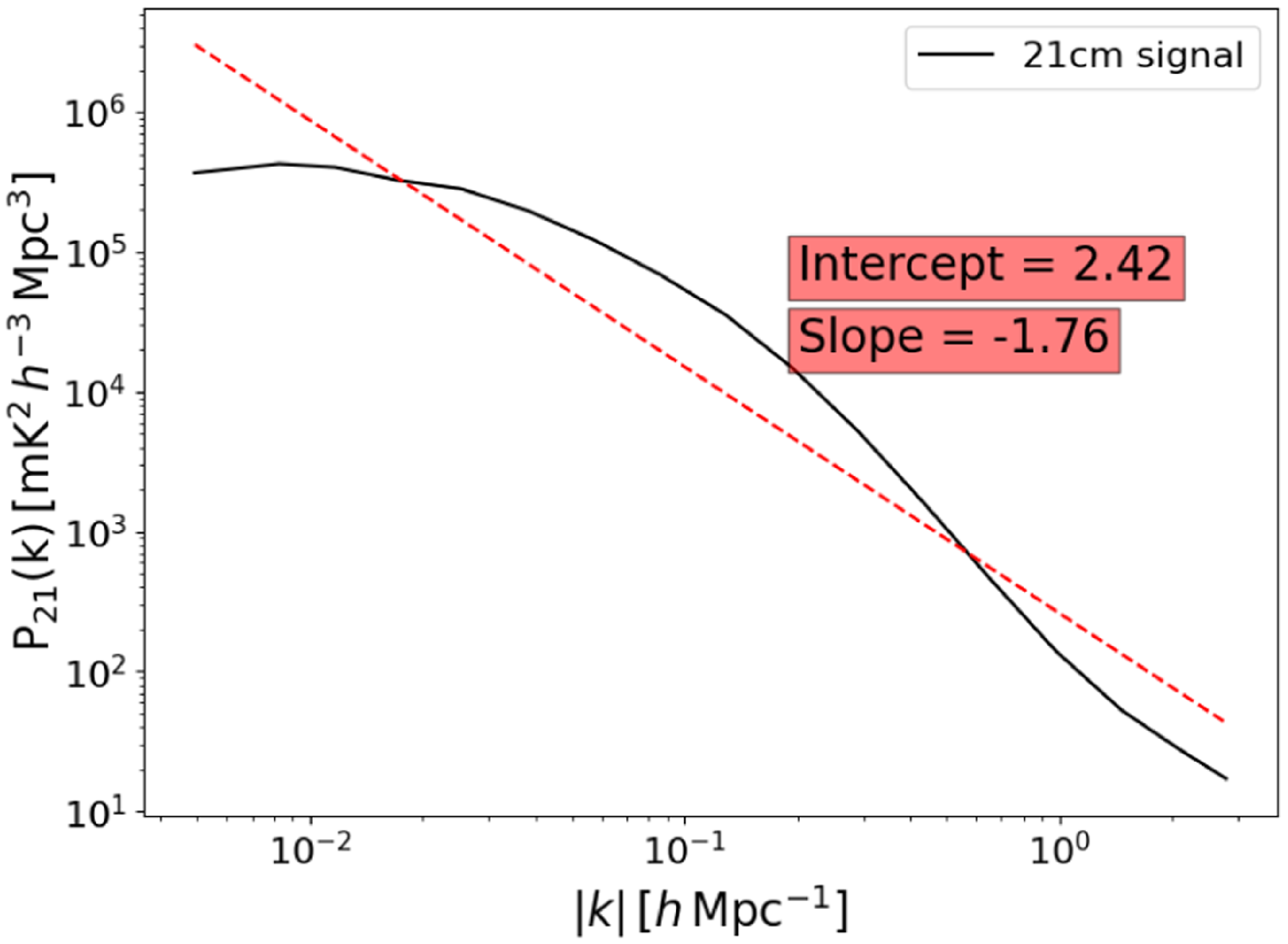
Figure 9. 21 cm signal at redshift
 $7.08$
obtained from 21CMFAST. The signal is fitted with a straight line of slope =
$7.08$
obtained from 21CMFAST. The signal is fitted with a straight line of slope =
 $-1.76$
and amplitude
$-1.76$
and amplitude
 $2.42$
.
$2.42$
.
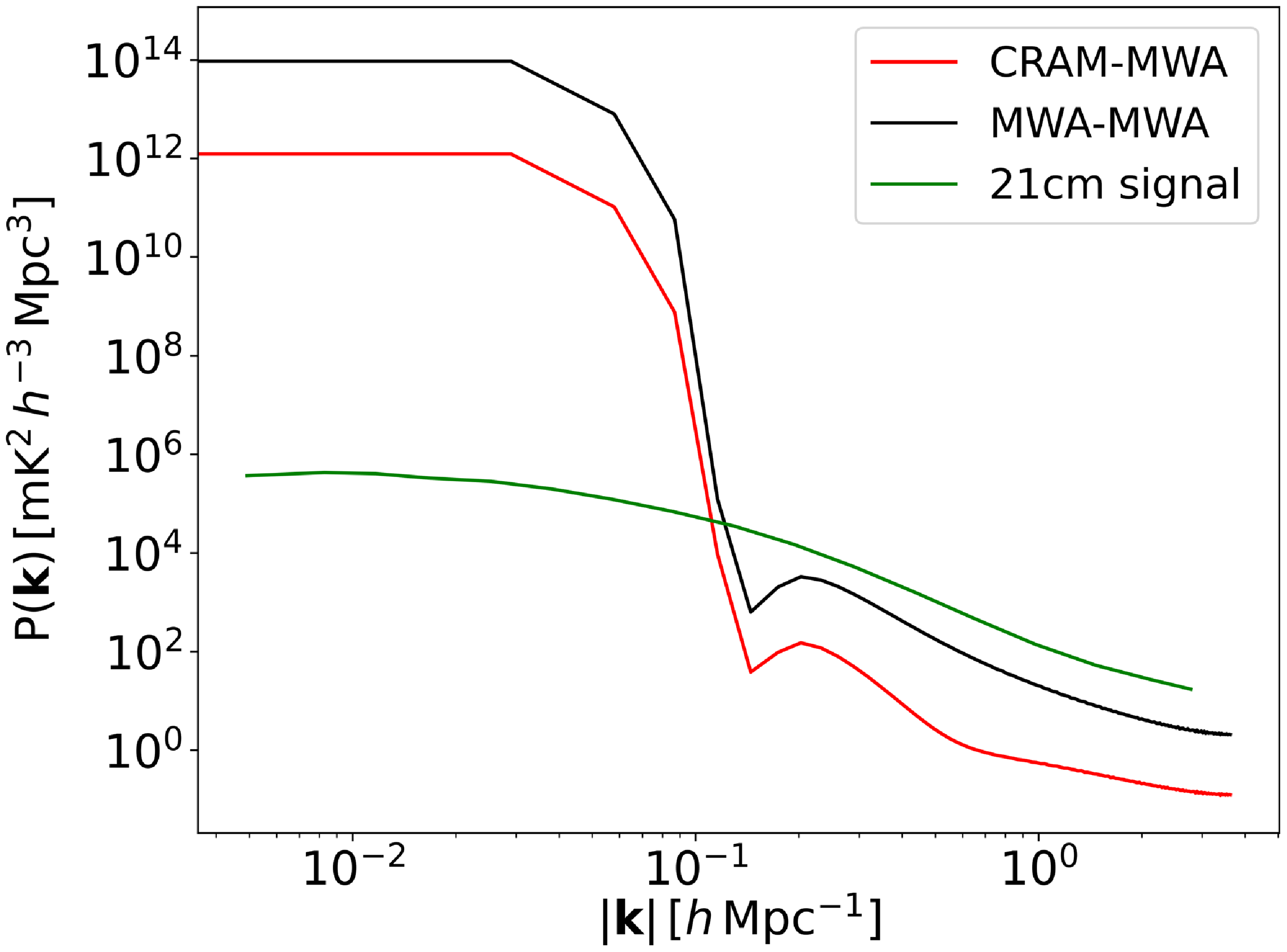
Figure 10. The power spectrum results for phase centre at
 $\mathrm{RA} = 12$
hrs 2 min are depicted, with the CRAM-MWA baseline shown in red and the MWA-MWA baseline in black along with the 21 cm signal shown in green. The CRAM-MWA baseline exhibits a reduced response, allowing access to additional k-modes of the 21 cm signal compared to the higher response obtained with MWA-MWA baselines.
$\mathrm{RA} = 12$
hrs 2 min are depicted, with the CRAM-MWA baseline shown in red and the MWA-MWA baseline in black along with the 21 cm signal shown in green. The CRAM-MWA baseline exhibits a reduced response, allowing access to additional k-modes of the 21 cm signal compared to the higher response obtained with MWA-MWA baselines.
6. Discussion
Instruments with a large FoV for the 21 cm experiments introduce wide-field effects, causing the bright radio foregrounds to overwhelm the weak cosmological signal. The results obtained in this work are in response to the challenges faced by the MWA telescope due to the large FoV of observation. This work demonstrates that utilising a larger tile configuration with a smaller FoV, such as the CRAM, can reduce the impact of foregrounds, as shown by the power spectrum results. The CRAM has a FoV half the MWA’s at every frequency under consideration while retaining the ability to measure the characteristic scale size of the cosmological signal. For the 21 cm experiments, it is an inherent challenge to simultaneously meet the requirements of sensitivity while suppressing the dominant foregrounds present in the datasets. Hence, the FoV opted for the experiment is a trade-off made towards the successful detection of the intended cosmic scale of the cosmological signal. With the larger tile configuration CRAM, the sidelobe response to the foregrounds near the horizon will be reduced and limit the leakage into the EoR window. Thus, using an instrument with a smaller FoV allows for accessing the k-modes near the wedge-EoR window boundary, where the cosmological signal is stronger. Thereby, CRAM aids the MWA telescope towards improving the probability of detecting the cosmological signal. The statistical analysis aimed at CRAM and MWA will aid the SKA era, which can have a hybrid array configuration (Barry et al. Reference Barry, Bernardi, Greig, Kern and Mertens2022).
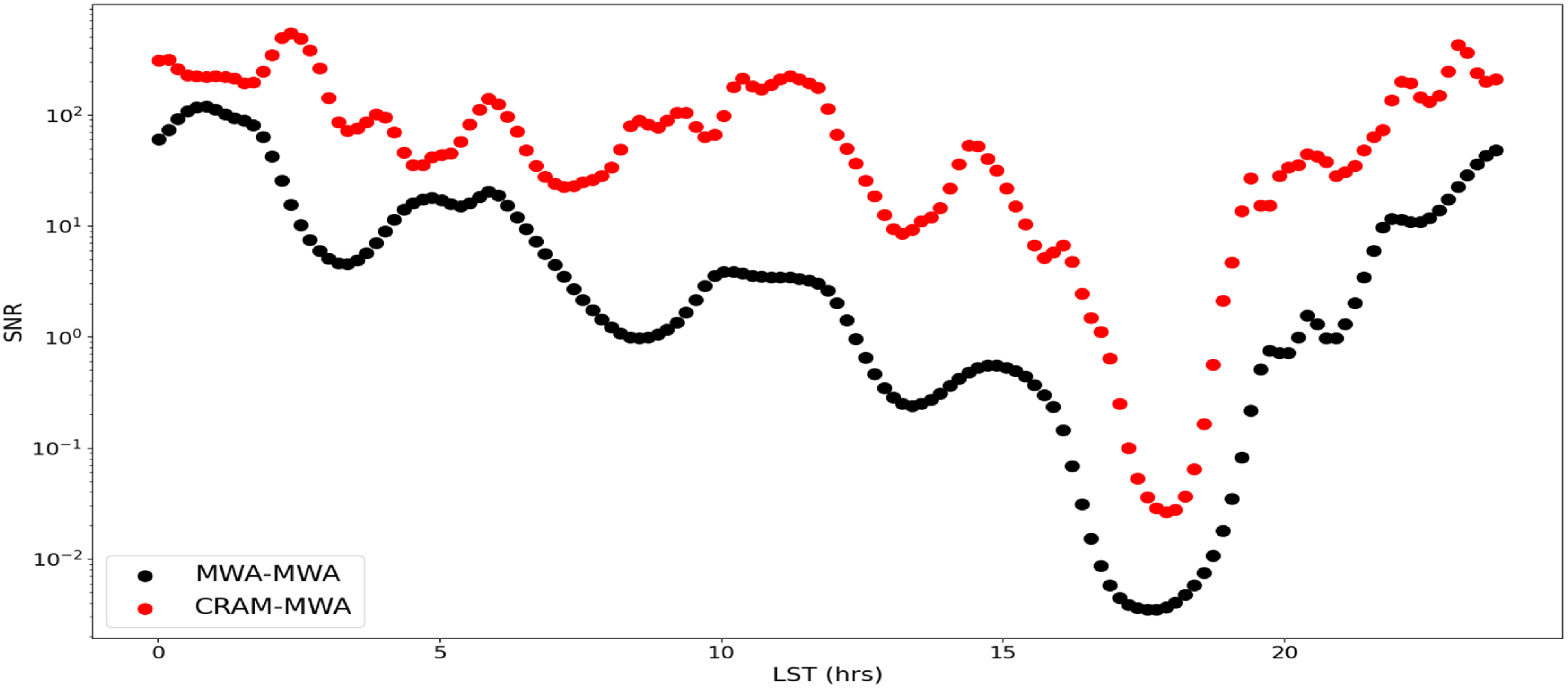
Figure 11. The SNR estimation on the slope of the 1D power spectrum, m, obtained for snapshots of the power spectrum across 24 hrs of observation. The red curve shows the SNR obtained using power spectrum results using CRAM-MWA baselines and the black curve shows the results obtained from MWA-MWA baselines. Across the 24 hrs of observations, the CRAM baselines have a larger SNR ratio indicating that the foregrounds have a lesser impact on instruments with smaller FoV. A similar plot is obtained for the SNR estimation of the amplitude of the 1D power spectrum.
The new instrument CRAM differs from a regular MWA tile in physical size and pointing direction, necessitating different data processing and calibration techniques compared to the MWA telescope. Typically, MWA visibility data are gridded using a gridding kernel of choice (typically Gaussian kernel or Blackman-Harris) in the uv-plane before estimating the cylindrical and spherical power spectrum. With CRAM, we obtain just 128 baseline combinations with the regular MWA Phase II configuration. The resulting uv-plane obtained is not filled to coherently add power to all k-modes. Thus, gridding introduces signal loss in power spectrum results, especially obtained with the CRAM baselines. This loss is less apparent for foregrounds, especially at the edge of the wedge, as the foreground power is a result of the leakage from the wedge into the EoR window. On the contrary, for a simulated 21 cm signal, the edge of the wedge has real power. Hence, with the gridding of a poorly represented uv-plane, the power of the 21 cm signal is lost. Line et al. (Reference Line2024) recognise this issue and devise a correction factor to compensate for the signal loss caused by gridding. On the contrary, with the delay spectrum technique, the power is intact without any loss and enables a direct comparison of power on individual baselines between the two configurations. With CRAM positioned within the compact array, creating redundant groups with MWA tiles, a direct comparison of power between MWA-MWA and CRAM-MWA redundant groups can be advantageous for statistically analysing real data for EoR science.
This work acknowledges that we have only used a simple analytical beam model for MWA and CRAM, as in Paper I, rather than the full EM simulation. The primary reason for not opting to use the full EM simulation as often used in the MWA EoR science is that this is proof of concept work that requires a beam model as simple as the analytical model to verify and validate the pipeline. Nevertheless, we expect to develop a full EM model of the CRAM for future work.
This work currently utilises visibilities obtained from simulated sky models to estimate the power spectrum results, demonstrating CRAM’s enhanced performance in mitigating foregrounds. In the future, we intend to utilise real data from the instrument to test the pipeline developed in this work. Furthermore, we intend to utilise the correlated real visibilities obtained with the CRAM-MWA baselines and develop statistical methods to improve MWA-EoR science. The instrument is currently active for scientific observations, with zenith-only pointing to align with MWA’s observations, avoiding the Galactic plane overhead.
7. Conclusion
In this work, we developed a proof of concept with the new instrument, the CRAM, a larger tile consisting of
 $8 \times 8$
dipoles installed within the MWA Phase II configuration. The CRAM has a smaller FoV at every frequency under consideration and a reduced sidelobe response when compared to the regular MWA. Employing an instrument with a smaller FoV can be beneficial for EoR science as the impact of foregrounds will be attenuated in accordance with the reduced primary beam response of the instrument.
$8 \times 8$
dipoles installed within the MWA Phase II configuration. The CRAM has a smaller FoV at every frequency under consideration and a reduced sidelobe response when compared to the regular MWA. Employing an instrument with a smaller FoV can be beneficial for EoR science as the impact of foregrounds will be attenuated in accordance with the reduced primary beam response of the instrument.
To demonstrate, we developed a power spectrum pipeline for the hybrid setup of MWA and CRAM. Employing a drift scanning strategy, the pipeline computes the 2D and 1D power spectrum for a series of two-minute observations, where the phase centre remains constant in the middle of the scan (HA =
 $\pm 1$
) and the beam pointing centre at the zenith. Using a simulated point source sky model, we demonstrate that when the phase centre of observation is at the zenith, both the baseline configurations have equal power of foregrounds in the DC mode of the 2D power spectrum as it is normalised by the volume. Further, by using EDA2 sky maps, we demonstrated using simulations that the power spectrum (both 2D and 1D) obtained using CRAM baseline configuration has a reduced response in power across the full 24 hrs of observation when compared to the power spectrum results obtained with the regular MWA baselines. This is further confirmed by the Fisher analysis conducted with the 21 cm signal and foreground estimations of power spectrum results obtained with the two baseline configurations. The SNR estimations of the slope and amplitude of the 1D power spectrum confirm an enhanced signal detection performance with the CRAM-MWA baselines. The reduction in foreground power obtained with the CRAM is due to the instrument’s reduced FoV and the smooth spectral nature of the foregrounds. However, the reduction in the FoV does not impact the isotropic 21 cm signal. The pipeline is further tested with a simulated 21 cm signal to demonstrate that the two pipelines can achieve equivalent power spectrum results for a simulated 21 cm signal. The equivalent power obtained confirms that the pipeline developed with the hybrid setup is reliable in differentiating the spectral nature of the signal.
$\pm 1$
) and the beam pointing centre at the zenith. Using a simulated point source sky model, we demonstrate that when the phase centre of observation is at the zenith, both the baseline configurations have equal power of foregrounds in the DC mode of the 2D power spectrum as it is normalised by the volume. Further, by using EDA2 sky maps, we demonstrated using simulations that the power spectrum (both 2D and 1D) obtained using CRAM baseline configuration has a reduced response in power across the full 24 hrs of observation when compared to the power spectrum results obtained with the regular MWA baselines. This is further confirmed by the Fisher analysis conducted with the 21 cm signal and foreground estimations of power spectrum results obtained with the two baseline configurations. The SNR estimations of the slope and amplitude of the 1D power spectrum confirm an enhanced signal detection performance with the CRAM-MWA baselines. The reduction in foreground power obtained with the CRAM is due to the instrument’s reduced FoV and the smooth spectral nature of the foregrounds. However, the reduction in the FoV does not impact the isotropic 21 cm signal. The pipeline is further tested with a simulated 21 cm signal to demonstrate that the two pipelines can achieve equivalent power spectrum results for a simulated 21 cm signal. The equivalent power obtained confirms that the pipeline developed with the hybrid setup is reliable in differentiating the spectral nature of the signal.
Acknowledgement
This research was partly supported by the Australian Research Council Centre of Excellence for All Sky Astrophysics in 3 Dimensions (ASTRO 3D), through project number CE170100013. CMT was supported by an ARC Future Fellowship under grant FT180100321. The International Centre for Radio Astronomy Research (ICRAR) is a joint venture between Curtin University and The University of Western Australia, funded by the Western Australian State government. This scientific work uses data obtained from Inyarrimanha Ilgari Bundara, CSIRO’s Murchison Radio-astronomy Observatory. We acknowledge the Wajarri Yamaji People as the Traditional Owners and native title holders of the Observatory site. The establishment of CSIRO’s Murchison Radio-astronomy Observatory is an initiative of the Australian Government, with support from the Government of Western Australia and the Science and Industry Endowment Fund. Support for the operation of the MWA is provided by the Australian Government (NCRIS) under a contract to Curtin University administered by Astronomy Australia Limited. This work was supported by resources provided by the Pawsey Supercomputing Research Centre with funding from the Australian Government and the Government of Western Australia. We would like to acknowledge Dr Jack Line for the valuable discussions regarding the 21 cm light cone simulations integrated into this work.
Data Availability
Data and code used to produce this work will be made available upon suitable requests.
Appendix A. Fisher Matrix derivation
Characterising the fiducial 21 cm signal after converting to cosmological units as a straight line is given as
 \begin{align} \log_{10}P_{21}(k) &= m\log_{10}k + C, \end{align}
 \begin{align} P_{21}(k) = 10^Ck^{m}.\end{align}
We formulate the Fisher matrix based on these parameters of the straight line using Equation (7) and is given by
 \begin{equation}\textbf{F}_{m,\,C} =10^C\begin{bmatrix} \displaystyle\sum_{i\in k}\dfrac{(\ln k_{i})^2 k_{i}^m}{\sigma^{2}_{i}}& \ln 10\displaystyle\sum_{i\in k}\dfrac{k_{i}^m \ln k_{i}}{\sigma^{2}_{i}} \\ \ln 10\displaystyle\sum_{i\in k}\dfrac{ k_{i}^m \ln k_{i}}{\sigma^{2}_{i}} & (\ln 10)^2\displaystyle\sum_{i\in k}\dfrac{ k_{i}^m}{\sigma^{2}_{i}} \\\end{bmatrix},\end{equation}
where
 $\sigma_{i}$
is the foreground power calculated using the spherically averaged power spectrum for a given instrument setup. The covariance matrix is the inverse of the Fisher matrix.
$\sigma_{i}$
is the foreground power calculated using the spherically averaged power spectrum for a given instrument setup. The covariance matrix is the inverse of the Fisher matrix.


 Open access