


1. Introduction
We are concerned with the asymmetric oscillation

where $x^+=\max \{x,\, 0\},$ $x^{-}=\max \{-x,\, 0\},$
 $a,\, b$
 are two different positive constants, and $f(t)$
 is a $2\pi$
 -periodic function.
This equation models the suspension bridge [Reference Lazer and McKenna8] and has been widely studied. Fuçik [Reference Fuçik3] and Dancer [Reference Dancer2] studied it in their investigations of boundary value problems associated to equations with ‘jumping nonlinearities’. For recent developments, one can refer to [Reference Gallouet and Kavian4, Reference Habets, Ramos and Sanchez5, Reference Lazer and McKenna7, Reference Zhang16] and the references therein.
For Littlewood's boundedness problem of the asymmetric oscillation (1.1), the earliest contribution was due to Ortega [Reference Ortega12]. In 1996, he considered the equation

where the smooth function $h(t)$ is $2\pi$
 -periodic. He proved that if $|\varepsilon |$
 is sufficiently small, then all solutions are bounded. That is, if $x(t)$
 is a solution, then it is defined for all $t\in \mathbb {R}$
 and
and

This result is in contrast with the well-known phenomenon of linear resonance that occurs in the case $a=b=n^2.$ For example, for any $\varepsilon \neq 0,$
 all solutions of

are unbounded.
For the asymmetric oscillation (1.1). Let $\omega _0:=\frac {1}{2}(\frac {1}{\sqrt {a}}+\frac {1}{\sqrt {b}})$ .
.
If $\omega _0\in \mathbb {R}\backslash \mathbb {Q},$ Ortega [Reference Ortega14] in 2001 proved the boundedness of all solutions of equation (1.1) under the condition $\int _0^{2\pi }f(t){\rm d}t\neq 0.$
Recently, Hu et al. [Reference Hu, Liu and Liu6] established an invariant curve theorem and applied it to equation (1.1), then they obtained the boundedness of all solutions with $\omega _0$ satisfying the Diophantine condition, but without the assumption $\int _0^{2\pi }f(t){\rm d}t\neq 0$
 .
.
Subsequently, we [Reference Li and Li10] also proved the boundedness of all solutions of equation (1.1) without the assumption $\int _0^{2\pi }f(t){\rm d}t\neq 0$ , but $\omega _0$
 is assumed to satisfy an approximation function condition.
If $\omega _0\in \mathbb {Q}$ , then there exist two positive integers $m$
 and $n$
 such that

Moreover, $m$ and $n$
 are relatively prime.
Denote by $C(t)$ the solution of the ‘homogeneous’ equation

with the initial conditions $C(0)=1,\, C'(0)=0$ . Then it is well known that $C(t)\in C^2(\mathbb {R})$
 and can be given explicitly by the formula

Denote the derivative of $C$ by $S=C'$
 , then $S(t)\in C(\mathbb {R})$
 and
and
(1) $C(-t)=C(t),\, ~S(-t)=-S(t)$
 ;
;(2) $C(t)$
and $S(t)$ are $2\pi \frac {m}{n}$-periodic functions;(3) $S(t)^2+a\,C^+(t)^2+b\,C^{-}(t)^2\equiv a$
.


For a given $2\pi$ -periodic function $f(t).$
 Let
Let

and

Then $\Phi _f(\theta )$ is a $2\pi$
 -periodic function and its derivative is

On the one hand, if $\mathcal {A}=\emptyset,$ Liu [Reference Liu11] in 1999 proved that all solutions of equation (1.1) are bounded. On the other hand, if $\mathcal {A}\neq \emptyset$
 and all zeros of $\Phi _f(\theta )$
 are non-degenerate, that is, $\Phi _f'(\theta )\neq 0$
 for all $\theta \in \mathcal {A},$
 Alonso and Ortega [Reference Alonso and Ortega1] in 1998 proved that there exists $R>0$
 such that every solution of (1.1) with

for some $t_0\in \mathbb {R}$ is unbounded. Particularly, the proof of this result implies that if there is a non-degenerate zero of $\Phi _f(\theta )$
 , then there exist unbounded solutions of equation (1.1). We remark that the references [Reference Liu11] and [Reference Alonso and Ortega1] assume that $\Phi _f(\theta )\not \equiv 0$
 .
.
In 1998, Ortega [Reference Ortega13] proposed an example

In this example, $\omega _0=3/4$ . Hence, the results of [Reference Alonso and Ortega1] and [Reference Liu11] can be applied. If $|\lambda |<1/45,$
 then all solutions with large initial conditions are unbounded. If $|\lambda |>1/45,$
 then all solutions are bounded.
However, when $|\lambda |=1/45,$ all zeros of $\Phi _f(\theta )$
 are degenerate. Therefore, the references [Reference Alonso and Ortega1] and [Reference Liu11] can not be applied to this equation. In 2021, we [Reference Li and Li9] proved the existence of unbounded solutions of equation (1.3) with $\lambda =\pm 1/45$
 .
.
The main idea of [Reference Li and Li9] is as follows. First, the corresponding Poincaré map in action and angle variables can be expressed by

Then in equation (1.3) with $\lambda =\pm \frac {1}{45},$ for all $\theta ^*\in \mathcal {A},$
 we have $\Phi _f(\theta ^*)=\Phi _f'(\theta ^*)=0.$
 Thus, $\mu _1(\theta )$
 has only degenerate zeros. However, in these two examples, the function $p(\theta,\, r):=\mu _1(\theta )+\frac {1}{r}k_1(\theta )+\frac {1}{r^2}h_1(\theta )$
 has some non-degenerate zeros. Then an invariant set near the zero of $\mu _1(\theta )$
 can be found, and each solution starting from this invariant set is unbounded.
Unfortunately, this method to find the invariant set depends on the property that the function $p(\theta,\, r)$ has non-degenerate zero, and cannot deal with the other cases, including that all zeros of $p(\theta,\, r)$
 are degenerate, or $p(\theta,\, r)$
 has no zero. In this paper, we will obtain the existence of unbounded solutions of equation (1.1) without considering the zero of $p(\theta,\,r).$
 More precisely, we will prove
Theorem 1.1 Assume that the resonance condition (1.2) holds, $f(t)$ is a real analytic $2\pi$
 -periodic function such that $\Phi _f(\theta )\not \equiv 0$
 and $\mathcal {A}(f)\neq \emptyset$
 . Then equation (1.1) has unbounded solutions.
Remark 1.2 When $\Phi _f(\theta )\not \equiv 0$ , if $\mathcal {A}(f)=\emptyset$
 , then all solutions of equation (1.1) are bounded by [Reference Liu11]. If $\mathcal {A}(f)\not =\emptyset$
 , then equation (1.1) has unbounded solutions by theorem 1.1. Therefore, theorem 1.1 together with the result of [Reference Liu11] completely solves Littlewood's boundedness problem for the asymmetric oscillation (1.1) in the resonance case under the assumption $\Phi _f(\theta )\not \equiv 0$
 .
.
In fact, according to the result of Alonso and Ortega in [Reference Alonso and Ortega1], here we only need to consider the situation that for all $\theta ^*\in \mathcal {A}(f),$ $\Phi _f'(\theta ^*)=0$
 . The main idea for proving theorem 1.1 is similar to [Reference Xing, Wang and Wang15] and as follows. By means of a series of transformations, the original system is transformed into a normal form, for which the twist condition is violated. Then an invariant set will be found, and each solution starting from the invariant set is unbounded.
The rest of this paper is organized in 4 sections as follows. In § 2, we will give some examples to illustrate the main theorem. Section 3 is devoted to finding the transformations and the normal form (for which the twist condition is violated). Then in § 4, we will give some properties of the discriminative function $\Phi _f(\theta ),$ which is crucial in this paper. Finally, the proof of the existence of unbounded solutions will be given in § 5.
2. Some remarks
We give several examples to illustrate theorem 1.1. The first two examples show that theorem 1.1 is applicable.
Example 2.1 For equation (1.3) with $\lambda =\pm \frac {1}{45}$ , the discriminative function takes the form

In view of theorem 1.1, this equation has unbounded solutions, which is consistent with the result of [Reference Li and Li9].
Example 2.2 Consider the equation

The discriminative function of this equation takes the form

and the results of [Reference Alonso and Ortega1, Reference Liu11] and theorem 1.1 can be applied.
• When $\lambda _2=\lambda _3=0,$
the discriminative function is of the form
\[ \Phi_f(\theta)={-}4\lambda_1. \]If $\lambda _1\neq 0,$
then all solutions are bounded. If $\lambda _1=0,$ then equation (2.1) becomes
\[ x''+4x^+{-}x^-{=}0, \]and all solutions are bounded. Thus, when $\lambda _2=\lambda _3=0,$
all solutions of (2.1) are bounded.• When $\lambda _2=0,\, ~\lambda _3\neq 0,$
the discriminative function is of the form
\[ \Phi_f(\theta)={-}4\lambda_1-\frac{4}{45}\lambda_3\sin3\theta. \]If $\big |\frac {\lambda _1}{\lambda _3}\big |>\frac {1}{45},$
then all solutions are bounded. If $\big |\frac {\lambda _1}{\lambda _3}\big |<\frac {1}{45},$ then all solutions with large initial conditions are unbounded. If $\big |\frac {\lambda _1}{\lambda _3}\big |=\frac {1}{45},$ then equation (2.1) has unbounded solutions.• When $\lambda _2\neq 0,$
the discriminative function is of the form
\[ \Phi_f(\theta)={-}4\lambda_1+\frac{4}{45}\sqrt{\lambda_2^2+\lambda_3^2}\cos(3\theta+\alpha),~~\alpha=\arctan\frac{\lambda_3}{\lambda_2}. \]Thus, if $\Big |\frac {\lambda _1}{\sqrt {\lambda _2^2+\lambda _3^2}}\Big |>\frac {1}{45},$
then all solutions are bounded. If $\Big |\frac {\lambda _1}{\sqrt {\lambda _2^2+\lambda _3^2}}\Big |<\frac {1}{45},$ then all solutions with large initial conditions are unbounded. If $\Big |\frac {\lambda _1}{\sqrt {\lambda _2^2+\lambda _3^2}}\Big |=\frac {1}{45},$ then equation (2.1) has unbounded solutions.


Finally, for equation (1.1), when $\Phi _f(\theta )\equiv 0,$ there are no results which can be applied to determine the boundedness of its solutions. The following examples show that this situation can indeed happen.
Example 2.3 Consider the equation

where the resonance condition (1.2) holds, $a\neq b$ and $r$
 is a positive integer. Then the discriminative function is

and it is easy to see that when $\frac {rn}{\sqrt {a}}$ is odd, we have $\Phi _f(\theta )\equiv 0.$
Example 2.4 Consider the equation

where $k$ is a positive integer. Then the discriminative function is

Thus, if $k=4r,\, r=1,\,2,\,3,\,\ldots,$ then
then

and if $k\neq 4r,\, r=1,\,2,\,3,\,\ldots,$ then $\Phi _f(\theta )\equiv 0.$
3. Transformations
We make a series of canonical transformations to obtain a normal form for which the twist condition is violated.
3.1 Action and angle variables
Let $y=x'$ , then equation (1.1) is equivalent to the following planar system

The following result is standard.
Lemma 3.1 For any $(x_0,\, y_0)\in \mathbb {R}^2$ and $t_0\in \mathbb {R},$
 the unique solution $z(t)=(x(t; t_0,\, x_0,\, y_0),\, y(t; t_0,\, x_0,\, y_0))$
 of (3.1) satisfying $z(t_0)=(x_0,\, y_0)$
 exists on the whole $t$
 -axis.
For $r>0,\, \theta \,(\text {mod}~2\pi ),$ define the following generalized polar coordinates $\Gamma :(r,\, \theta )\rightarrow (x,\, y)$
 by
by

where $\rho :=\sqrt {\frac {2n}{am}}$ . It is easy to check that $\Gamma$
 is a symplectic transformation.
The Hamiltonian associated to the system (3.1) is expressed in Cartesian coordinates by

In the new coordinates $(r,\, \theta ),$ it becomes

Thus, the system (3.1) is transformed into

which is a semilinear system.
3.2 A sublinear system
First, introduce a new time variable $\vartheta$ by $t=m\vartheta$
 to eliminate the denominator of the linear part of (3.2). Then, the system (3.3) is transformed into

where

For convenience, we can rewrite (3.5) and (3.4) respectively as

and

Since $m$ is a positive integer, then the new Hamiltonian $H(r,\, \theta,\, t)$
 in (3.6) is $2\pi$
 -periodic in $\theta$
 and $t.$
Next we introduce a rotation transformation to eliminate the linear part of the Hamiltonian (3.6), which helps us to obtain a sublinear system.
Define the rotation transformation $\Phi _1: (r_1,\, \theta _1,\, t)\rightarrow (r,\, \theta,\, t)$ by
by

Then under $\Phi _1,$ the original semilinear system determined by the Hamiltonian (3.6) is transformed into a sublinear system given by the following Hamiltonian

It is worth to point out that the above transformations preserve the periodicity and boundedness of solutions. In fact, if $(r_1(t+2\pi ),\, \theta _1(t+2\pi ))=(r_1(t),\, \theta _1(t))$ , then for the Hamiltonian (3.5), $r(\vartheta +2\pi )=r_1(\vartheta +2\pi )=r_1(\vartheta )=r(\vartheta )$
 , and $\theta (\vartheta +2\pi )=\theta _1(\vartheta +2\pi )+n(\vartheta +2\pi )=\theta _1(\vartheta )+n\vartheta +2n\pi =\theta (\vartheta )+2n\pi$
 . Since $t=m\vartheta,$
 for the Hamiltonian (3.2), we have $r(\frac {1}{m}t+2\pi )=r(\frac {1}{m}t),$
 and $\theta (\frac {1}{m}t+2\pi )=\theta (\frac {1}{m}t)+2n\pi.$
 Thus for the original system (3.1), $x(\frac {1}{m}t+2\pi )=\rho r(\frac {1}{m}t+2\pi )^{\frac {1}{2}}C(\frac {m}{n}\theta (\frac {1}{m}t+2\pi ))=\rho r(\frac {1}{m}t)^{\frac {1}{2}}C(\frac {m}{n}\theta (\frac {1}{m}t)+2m\pi )=x(\frac {1}{m}t)$
 , which leads to ${x(t+2\pi )=x(t)}$
 . Thus, the periodicity is preserved. Similarly, it is easy to verify that the boundedness is also preserved.
3.3 The normal form without the twist condition
To reduce the power of term containing $t$ in the Hamiltonian (3.7), we make the transformation $\Phi _2: (r_2,\, \theta _2,\, t)\rightarrow (r_1,\, \theta _1,\, t)$
 given by

with the generating function $S_2(r_2,\, \theta _1,\, t)$ determined by

where

Under $\Phi _2,$ the Hamiltonian $H_1$
 in (3.7) is transformed into

It is obvious that

and thus,

Then by $\theta _2=\theta _1+\frac {\partial S_2}{\partial r_2}(r_2,\, \theta _1,\, t),$ we get

where

and

with

Then we have the following estimates, and the proof is elementary.
Lemma 3.2 For $r_2$ large enough, $\theta _2,\, t\in \mathbb {S}^1=\mathbb {R}/(2\pi \mathbb {Z}),$
 we have

and

where $C$ is a constant larger than 1.
Finally, with the definitions of $\Phi _f(\theta )$ and $[Cf](\frac {m}{n}\theta ),$
 $[Sf](\frac {m}{n}\theta )$
 , the Hamiltonian $H_2(r_2,\, \theta _2,\, t)$
 in (3.8) can be rewritten as

and for $r$ large enough, $\theta,\, t\in \mathbb {S}^1,$
 one has

where $C$ is a constant larger than 1.
4. Some properties of $\Phi _f(\theta )$

We present several lemmas for the discriminative function $\Phi _f(\theta )$ , which will be used in the proof of the existence of unbounded solutions.
First, we prove that under the assumptions of theorem 1.1, $\Phi _f(\theta )$ is an analytic function, and thus for any $\theta ^*\in \mathcal {A}$
 , there exists an integer $k\geq 2$
 such that ${\Phi _f^{(k)}(\theta ^*)\neq 0}$
 .
.
Lemma 4.1 Under the assumptions of theorem 1.1, for any $\theta ^*\in \mathcal {A},$ there exists an integer $k\geq 2$
 such that $\Phi _f(\theta ^*)=\Phi _f'(\theta ^*)=\cdots =\Phi _f^{(k-1)}(\theta ^*)=0,$
 $\Phi _f^{(k)}(\theta ^*)\neq 0.$
Proof. Since $f$ is real analytic and $2\pi$
 -periodic in $t$
 , then it can be written as a uniformly convergent Fourier series

where the Fourier coefficients

Moreover, $f$ can be analytically extended into a complex domain ${\{t\in \mathbb {C}:|\mathrm {Im} t|\leq r\}}$
 , with $r>0$
 a small constant, and we have $|f_k|\leq \|f\|_re^{-|k|r},$
 where $\|f\|_r=\sup _{|\mathrm {Im} t|\leq r}|f(t)|.$
Then it is obvious that the series

is also uniformly convergent to $C(\frac {m}{n}\theta +mt)f(mt)$ . Thus,

where

The periodicity of $C$ and $f$
 yields that

where

By some calculations, when $k=\pm \sqrt {a},$ we get

When $k=\pm \sqrt {b},$ similarly we have

When $k\neq \pm \sqrt {a},\, \pm \sqrt {b},$ we also obtain

Thus, for all $k\in \mathbb {Z},$ $\Phi _{ak}(\theta )$
 can be analytically extended to $\tilde {\Phi }_{ak}(\theta )$
 in $\{\theta \in \mathbb {C}: |\operatorname {Im}\theta |< r'\},$
 with $r'\leq r\frac {n}{m}$
 , and it is easy to see that

Similarly, for all $k\in \mathbb {Z},$ $\Phi _{bk}(\theta )$
 can also be analytically extended to $\tilde {\Phi }_{bk}(\theta )$
 in $\{\theta \in \mathbb {C}: |\operatorname {Im}\theta |< r'\},$
 and
and

Then with $|f_k|\leq \|f\|_re^{-|k|r},$ where $\|f\|_r=\sup _{|\mathrm {Im} t|\leq r}|f(t)|,$
 and since $r'\leq r\frac {n}{m}$
 , we have

By Weierstrass M-test, since the series $\sum \limits _{k\in \mathbb {Z}\atop k\neq \pm \sqrt {a},\, \pm \sqrt {b}}\frac {1}{|k^2-a||k^2-b|}$ is convergent, then in the domain $\{\theta \in \mathbb {C}: |\operatorname {Im}\theta |< r'\},$
 the series

uniformly converge to $\tilde {\Phi }_f(\theta )$ , which is a complex extension of $\Phi _f(\theta ).$
 Since all $\tilde {\Phi }_{ak}(\theta ),\, \tilde {\Phi }_{bk}(\theta )$
 are analytic, then by Weierstrass's Theorem, $\tilde {\Phi }_f(\theta )$
 is also analytic in the domain $\{\theta \in \mathbb {C}: |\operatorname {Im}\theta |< r'\}$
 .
.
Finally, under the assumptions of theorem 1.1, for any $\theta ^*\in \mathcal {A},$ we have $\tilde {\Phi }_f(\theta ^*)=\Phi _f(\theta ^*)=0,$
 $\tilde {\Phi }'_f(\theta ^*)=\Phi '_f(\theta ^*)=0.$
 Then with the isolation of zeros for analytic functions, for any $\theta ^*\in \mathcal {A},$
 there exists an integer $k\geq 2$
 such that $\tilde {\Phi }_f(\theta ^*)=\tilde {\Phi }_f'(\theta ^*)=\cdots =\tilde {\Phi }_f^{(k-1)}(\theta ^*)=0,$
 $\tilde {\Phi }_f^{(k)}(\theta ^*)\neq 0.$
 Thus, $\Phi _f(\theta ^*)=\Phi _f'(\theta ^*)=\cdots =\Phi _f^{(k-1)}(\theta ^*)=0,$
 $\Phi _f^{(k)}(\theta ^*)\neq 0.$
By lemma 4.1, choose some $\theta ^*\in \mathcal {A}.$ Without loss of generality, we can assume that $\Phi _f^{(k)}(\theta ^*)>0,$
 otherwise, make a time change $t\mapsto -t.$
In the following, for a fixed $\theta ^*\in \mathcal {A}$ and the corresponding integer $k\geq 2$
 , some estimates of $\Phi _f(\theta )$
 near $\theta ^*$
 are given.
Lemma 4.2 Assume that there exist $\theta ^*\in \mathbb {R}$ and $2\leq k\in \mathbb {N}$
 such that $\Phi _f(\theta ^*)=\Phi _f'(\theta ^*)=\cdots =\Phi _f^{(k-1)}(\theta ^*)=0,$
 $\Phi _f^{(k)}(\theta ^*)>0.$
 Then there exists $\delta _1>0$
 such that for all $\theta : 0<\theta -\theta ^*\leq \delta _1$
 , one has $\Phi _f(\theta )>0,\, \Phi _f'(\theta )>0.$
Proof. This lemma can be easily proved by properties of the derivative, so we omit the details here.
Let $\tau =\theta -\theta ^*.$ Then $\Phi _f(\theta )=\Phi _f(\tau +\theta ^*),$
 and we get the following lemma.
Lemma 4.3 Assume that there exists $2\leq k\in \mathbb {N}$ such that $\Phi _f(\theta ^*)=\Phi _f'(\theta ^*)=\cdots =\Phi _f^{(k-1)}(\theta ^*)=0,$
 $\Phi _f^{(k)}(\theta ^*)>0.$
 Then there exists $\delta _1>0$
 such that for all ${\tau : 0<\tau \leq \delta _1}$
 , we have $\Phi _f(\tau +\theta ^*)>0,\, \Phi _f'(\tau +\theta ^*)>0.$
Lemma 4.4 Assume that the function $g(x)$ is analytic at $x=0,$
 and ${g^{(j)}(0)=0,\,~j=0,\,1,\,\ldots,\,k-1,\, ~g^{(k)}(0)>0}$
 . Then there exists $\delta _2>0$
 such that for all $x: 0\leq x\leq \delta _2,$
 one has

where

Proof. On the one hand, let

Then $h_1(0)=h_1'(0)=\cdots =h_1^{(k-1)}(0)=0$ , and $h_1^{(k)}(0)=(1-c_1)g^{(k)}(0)=\frac {1}{6k+11} g^{(k)}(0)>0,$
 so there exists $\delta _3>0$
 such that for all $x: 0\leq x\leq \delta _3,$
 we have $h_1(x)\geq 0,$
 which leads to

On the other hand, let

Then $h_2(0)=h_2'(0)=\cdots =h_2^{(k-1)}(0)=0$ , and $h_2^{(k)}(0)=(1-c_2)g^{(k)}(0)=\frac {-1}{6k+11} g^{(k)}(0)<0,$
 so there exists $\delta _4>0$
 such that for all $x: 0\leq x\leq \delta _4,$
 we have $h_2(x)\leq 0,$
 which leads to

Let $\delta _2=\min \{\delta _3,\, \delta _4\}>0$ . Then for all $x: 0\leq x\leq \delta _2,$
 we have

where

Applying lemmas 4.1–4.4 to $\Phi _f(\tau +\theta ^*)$ and $\Phi _f'(\tau +\theta ^*).$
 Then we can easily obtain the following result.
Lemma 4.5 Under the assumptions of theorem 1.1, there exists $\delta >0$ such that for all $\tau : 0<\tau \leq \delta,$
 we have $\Phi _f(\tau +\theta ^*)>0,\, \Phi _f'(\tau +\theta ^*)>0,$
 and
and

where $c_1=\frac {6k+10}{6k+11}<1,\,~c_2=\frac {6k+12}{6k+11}>1.$
5. The existence of unbounded solutions
In this section, we prove that the Hamiltonian system with the Hamiltonian (3.9) has unbounded solutions.
The system with the Hamiltonian (3.9) is given by

Let $\tau =\theta -\theta ^*.$ Then the system (5.1) is transformed into

For fixed $2\leq k\in \mathbb {N}$ from lemma 4.1 and $\delta$
 from lemma 4.5, choose $r^*\gg 1$
 satisfying
(1) $r^*\gg \|f\|;$
(2) $2(r^*)^{-\frac {1}{3k}}<\delta$
;(3) $\frac {1}{3\pi }\frac {c_1}{(k-1)!}m\rho (\frac {r^*}{2})^{\frac {1}{2(2k-1)}}\Phi _f^{(k)}(\theta ^*)\geq 1,$
where $c_1=\frac {6k+10}{6k+11}.$


Give an initial point $(r(0),\, \tau (0))\in D:=\Big \{(r,\, \tau ):r^{-\frac {1}{2k-1}}\leq \tau \leq r^{-\frac {1}{3k}}\Big \}$ and $r(0)\geq r^*.$
First, the second equation in (5.2) implies that $\frac {{\rm d}r}{{\rm d}t}=O(r^{\frac {1}{2}}+1),$ thus $r(t)\geq \frac {1}{2}r^*$
 for any $t\in [0,\, 2\pi ]$
 by $r^*\gg \|f\|$
 . Also the first equation in (5.2) implies $\frac {{\rm d}\tau }{{\rm d}t}=O(r^{-\frac {1}{2}}),$
 hence $0<\tau (t)\leq 2(r^*)^{-\frac {1}{3k}}$
 for any $t\in [0,\,2\pi ].$
 Thus, lemma 4.5 can be applied in the following.
We claim that if the initial point $(r(0),\, \tau (0))\in D$ and $r(0)\geq r^*,$
 then $(r(t),\, \tau (t))\in D$
 for any $t\in [0,\, 2\pi ].$
 Otherwise, let $t_1:=\sup \{t: (r(s),\, \tau (s))\in D,\, ~0\leq s\leq t\}<2\pi.$
 It is obvious that $(r(t_1),\, \tau (t_1))\in \partial D,$
 which leads to $r(t_1)^l\tau (t_1)=1$
 with $l=\frac {1}{2k-1}$
 or $\frac {1}{3k}.$
By a direct computation, we get

Since $r(t_1)^l\tau (t_1)=1,$ $r(t)\geq \frac {1}{2}r^*$
 and $0<\tau (t)\leq 2(r^*)^{-\frac {1}{3k}}<\delta$
 for $t\in [0,\, 2\pi ]$
 , then we get

and

Now it is a position to apply lemma 4.5 to $J_1$ and $J_2.$
 On the one hand, if $l=\frac {1}{3k},$
 then we have

Since $c_1=\frac {6k+10}{6k+11}$ , $c_2=\frac {6k+12}{6k+11}$
 and $l=\frac {1}{3k},\, k\geq 2,$
 then $c_2l-\frac {c_1}{2k}<0,$
 $-\frac {3}{2}+l<-1<-\frac {1}{2}-l(k-1),$
 which lead to

That is, if $l=\frac {1}{3k},$ then $(r(t)^l\tau (t))'|_{t=t_1}<0.$
 Therefore, there exists $t_2>t_1$
 such that $r(t)^\frac {1}{3k}\tau (t)\leq 1$
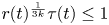 for $t\in [t_1,\, t_2],$
 which contradicts the definition of $t_1.$
 Thus for all $t\in [0,\, 2\pi ],$
 we have $\tau (t)\leq r(t)^{-\frac {1}{3k}}.$
On the other hand, if $l=\frac {1}{2k-1},$ then we have

Since $c_1=\frac {6k+10}{6k+11}$ , $c_2=\frac {6k+12}{6k+11}$
 and $l=\frac {1}{2k-1},\, k\geq 2,$
 then $c_1l-\frac {c_2}{2k}>0,$
 $-\frac {3}{2}+l<-1<-\frac {1}{2}-l(k-1),$
 which lead to

That is, if $l=\frac {1}{2k-1},$ then $(r(t)^l\tau (t))'|_{t=t_1}>0.$
 Therefore, there exists $t_2>t_1$
 such that $r(t)^\frac {1}{2k-1}\tau (t)\geq 1$
 for $t\in [t_1,\, t_2],$
 which contradicts the definition of $t_1.$
 Thus for all $t\in [0,\, 2\pi ],$
 one has $\tau (t)\geq r(t)^{-\frac {1}{2k-1}}.$
 The proof of the claim is completed.
Now we prove that every solution of system (5.2) with the initial point $(r(0),\, \tau (0))\in D$ and $r(0)\geq r^*$
 is unbounded.
From the claim, if the initial point $(r(0),\, \tau (0))\in D$ and $r(0)\geq r^*,$
 then for any $t\in [0,\, 2\pi ],$
 one has $r(t)^{-\frac {1}{2k-1}}\leq \tau (t)\leq r(t)^{-\frac {1}{3k}}\leq 2(r^*)^{-\frac {1}{3k}}.$
 Thus, from the second equation of (5.2), for any $t\in [0,\, 2\pi ],$
 we obtain

Choose $r^*$ sufficiently large such that $\frac {1}{3\pi }\frac {c_1}{(k-1)!}m\rho (\frac {r^*}{2})^{\frac {1}{2(2k-1)}}\Phi _f^{(k)}(\theta ^*)\geq 1.$
 Then $r(2\pi )\geq r(0)+2\pi >r^*.$
In a word, if $(r(0),\, \tau (0))\in D$ and $r(0)\geq r^*,$
 then $(r(2\pi ),\, \tau (2\pi ))\in D$
 and $r(2\pi )\geq r(0)+2\pi >r^*.$
Using the above argument repeatedly, if $(r(0),\, \tau (0))$ satisfies the above initial conditions, then $r(2\pi i)\geq r(0)+2\pi i$
 for any $i\in \mathbb {N},$
 which means that the solution $(r(t),\, \tau (t))$
 is unbounded. Up to now theorem 1.1 is proved.
Acknowledgements
X. Li was supported by NSFC (11971059).
