


Introduction
Subsidence is one of the processes influencing the dynamics of the Wadden Sea region. Together with sea-level rise, natural sediment transport, deposition, and erosion and induced sediment suppletion and sand extraction, subsidence directly affects the future of the area. The crucial variable in this context is the change of the relative sea level – the local sea level relative to the onshore land elevation (Van der Spek, Reference Van der Spek2018; Vermeersen et al., Reference Vermeersen2018; Wang et al., Reference Wang, Elias and van der Spek2018).
In this contribution we discuss subsidence in the context of the Dutch Wadden Sea. We start by describing the processes causing subsidence and how these can be modelled. For reliable forecasts, however, subsidence behaviour of the past must be known and understood. Monitoring is thus a crucial activity in this respect, and measurements must be understood in the context of the models by model calibration. These issues are the subject of the following sections.
Most human-induced subsidence in the Wadden Sea originates from gas production and salt mining. For individual fields, a lot of work has been done to forecast subsidence in the Wadden Sea by using more or less elaborate implementations of the modelling, measuring and calibration technology. For the Wadden Sea area, the forecasts must always be translated into an average value for each tidal basin in order to assess the impact on the larger Wadden Sea development. Further, they must always be accompanied by a quality measure. We bring together these numbers further below.
We conclude by highlighting the gaps in our knowledge of the subject and by sketching how we can move forward to improve our understanding and forecasting capabilities.
Causes of subsidence
Natural causes of subsidence
Natural subsidence refers to long-term movements, and, on a timescale of thousands of years, three contributions play an important role: compaction, postglacial isostacy and tectonics (Kooi et al., Reference Kooi, Johnston, Lambeck, Smither and Molendijk1998). When we measure surface movements the combined effects of these three contributions are detected. In the Netherlands, measurements of vertical land movement over the 20th century point to a regional slow tilting of the lithosphere, in a northwest–southeast direction (Fig. 1).
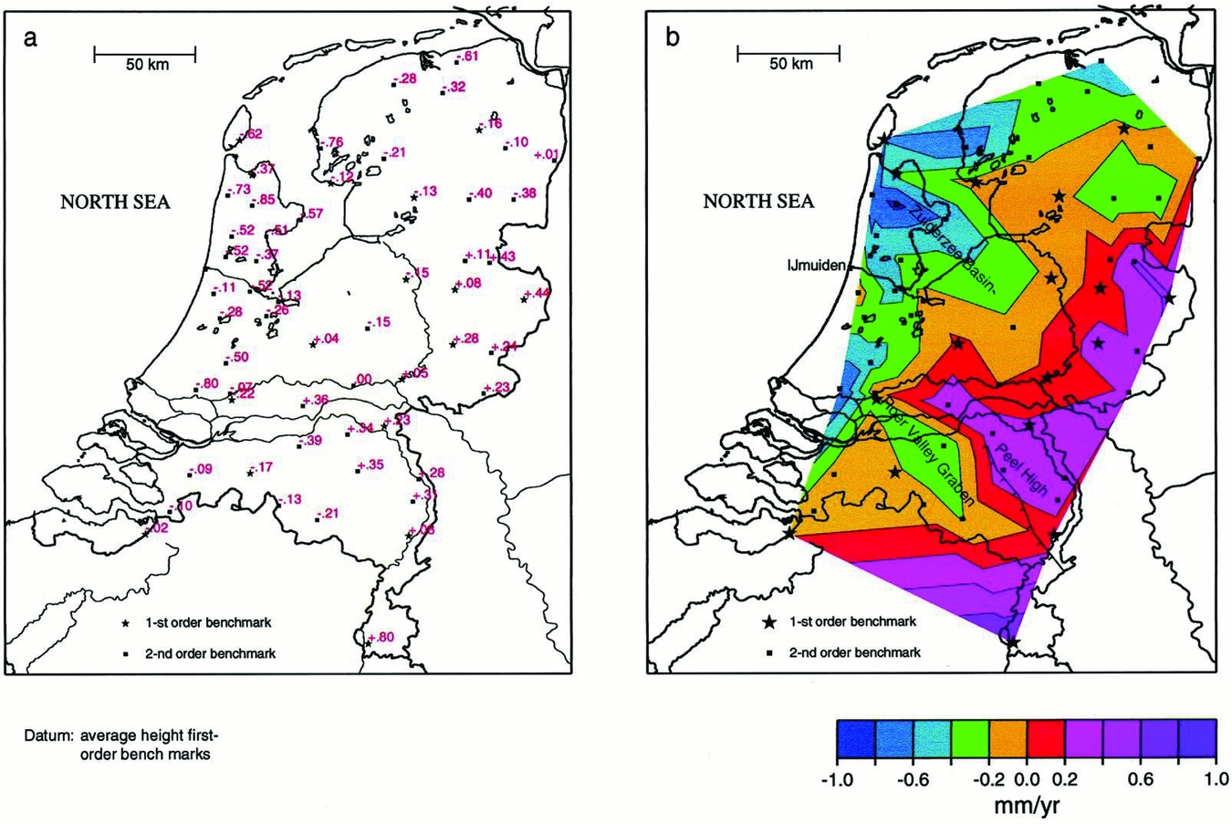
Fig. 1. Regional vertical land movement (mma−1) of top of the Pleistocene in the Netherlands obtained by least-squares kinematic adjustment of first- and second-order underground benchmarks. (a) Inferred rates of individual benchmarks. (b) Contour map of inferred rates. Minus sign denotes subsidence. Standard deviations vary between 0.1 and 0.3mma−1. (From Kooi et al., Reference Kooi, Johnston, Lambeck, Smither and Molendijk1998.)
Kooi et al. (Reference Kooi, Johnston, Lambeck, Smither and Molendijk1998) made an effort to quantify the three contributions to long-term subsidence in the Netherlands: compaction, postglacial isostasy and tectonics. The Netherlands are located at the southeast of the North Sea basin and at the mouth of major rivers, where sedimentary deposits have accumulated since the beginning of the Tertiary. The accumulating sediments cause compaction of the lower-lying strata.
Postglacial isostasy is the surface response caused by the reduction of load on it by melting of land ice. In the Netherlands, the effect of the melting of the glaciers in Scandinavia and Scotland has reduced gradually during the last 10,000 years (Lambeck & Chappell, Reference Lambeck and Chappell2001 and references therein; Kiden et al., Reference Kiden, Denys and Johnston2002; Peltier et al., Reference Peltier, Shennan, Drummond and Horton2002).
Tectonics in the Netherlands is operative predominantly in the rift system of the Roerdal graben, in the south of the country (Van Wees et al., Reference Van Wees, Buijze, van Thienen-Visser, Nepveu, Wassing, Orlic and Fokker2014). In this region, the Mw=5.8 magnitude earthquake in Roermond took place on 13 April 1992 (Van Eck & Davenport, Reference Van Eck and Davenport1994). Tectonic seismicity and related vertical land movement is not relevant in the Wadden Sea.
The disentanglement of the long-term surface movement into the three constituents since the Quaternary, as constructed by Kooi et al. (Reference Kooi, Johnston, Lambeck, Smither and Molendijk1998), is represented in Fig. 2. In the Wadden Sea, a slow, natural subsidence with expected velocities of less than 1mma−1 was estimated to take place until the present day. More information on natural processes of subsidence can be found in Vermeersen et al. (Reference Vermeersen2018).
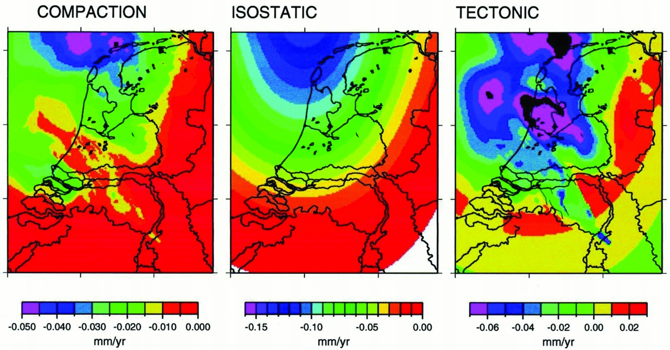
Fig. 2. Separation of compaction, isostatic and tectonic contributions to vertical land movement for the Quaternary (2.5Ma–present) constructed by three-dimensional backstripping of Cenozoic stratigraphy of the Netherlands and the southern North Sea basin (from Kooi et al., Reference Kooi, Johnston, Lambeck, Smither and Molendijk1998).
Anthropogenic causes of subsidence
Subsurface activities affecting the ground surface level in the Netherlands include the production of oil and gas, solution mining of salt, mining of coal (until the 1970s), gas storage and geothermal exploitation. Also, groundwater exploitation and peat oxidation have effects on the ground surface level (Van Asselen, Reference Van Asselen2010). For the Wadden Sea area, only the gas production and the salt mining activities are relevant.
Gas production implies the extraction of natural gas from a gas reservoir, which usually is a sandstone formation of which the pores contain the gas. The virgin pressure of the gas is of the order of the hydrostatic pressure of water at that depth, since there is pressure communication with water in the surrounding aquifers. The gas has accumulated and stayed in the reservoir over geological times thanks to a stratigraphic or structural trap. If a well is drilled from the surface into the reservoir, the high reservoir gas pressure causes the gas to flow up the well to the surface, where the well is coupled to the surface grid for the transport of natural gas to consumers.
The production of gas causes the pressure in the reservoir to drop. This leads to an increase in the effective stress that is operative between the grains in the matrix structure. Increased effective stresses cause a compaction of the reservoir. The process is indicated in Fig. 3.
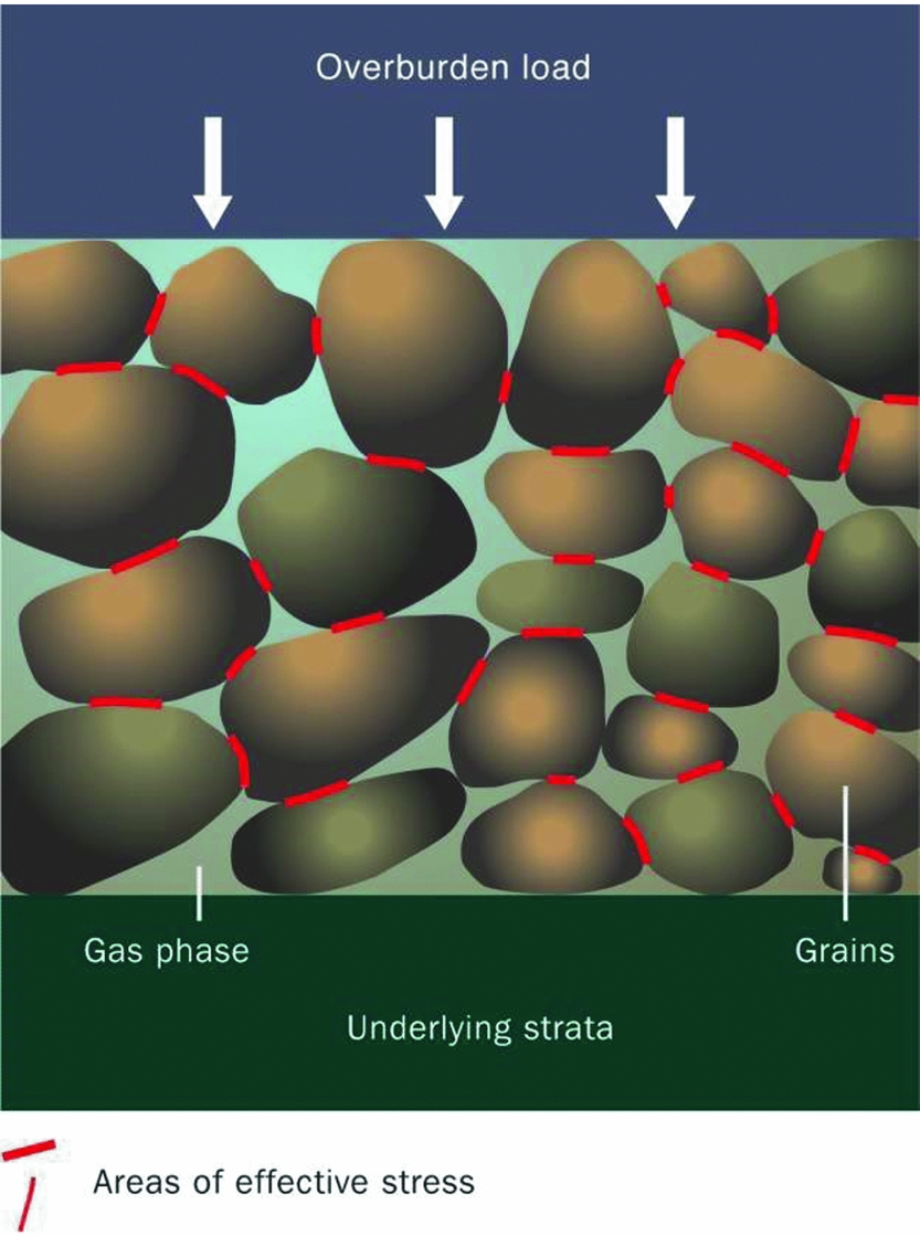
Fig. 3. Reservoir compaction as a result of reducing gas pressure (from De Waal et al., Reference De Waal, Roest, Fokker, Kroon, Muntendam-Bos, Oost and van Wirdum2012)
The mechanical response of the subsurface formations surrounding the compacting reservoir propagates the compaction of the reservoir to surface subsidence. The magnitude and extent of this movement depend, among other things, on the depth, the size and the shape of the gas field, the amount of gas produced and the associated pressure drop, possible depletion of connected aquifers, the mechanical properties of the reservoir rock and its geological structure, and the properties of the formations above, below and beside the reservoir (see e.g. Geertsma, Reference Geertsma1973a; Morton et al., Reference Morton, Bernier and Barras2006; De Waal et al., Reference De Waal, Roest, Fokker, Kroon, Muntendam-Bos, Oost and van Wirdum2012; Van Thienen-Visser & Fokker, Reference Van Thienen-Visser and Fokker2017 and references therein). The next section describes in more detail how these processes can be understood.
Salt solution mining is a technology to produce salt from deep rock salt layers. A well is drilled into the rock salt strata, then fresh water is pumped into this well, causing salt to dissolve and a cavern containing brine to develop. This brine is produced to the surface, where the salt is separated and brought to the market. In the salt caverns the brine pressure is kept below the lithostatic pressure. As a result, the elasto-visco-plastic salt flows toward the cavern. This is called squeeze mining (Fig. 4). After some time, typically 2–3 years, a dynamic balance develops between cavern volume increase due to the solution process and decrease due to convergence by the creep of salt. Volume and shape of the cavern then stay roughly constant. This method facilitates the production of large volumes of salt from caverns that remain limited in volume. The cavern convergence induces elastic deformation of the strata around it, which results in surface subsidence. Shape and magnitude of the subsidence bowl depend on the squeeze volume and the properties of the surrounding formations (Spiers et al., Reference Spiers, Schutjens, Brzesowsky, Peach, Liezenberg and Zwart1990; Fokker & Kenter, Reference Fokker and Kenter1994; Urai et al., Reference Urai, Schléder, Spiers, Kukla, Littke, Bayer, Gajewski and Nelskamp2008; Van Noort et al., Reference Van Noort, Drijkoningen, Arts, Thorbecke, Bullen and Visser2009; Hulscher et al., Reference Hulscher, Meire, Rienstra and Urai2016; Den Hartogh et al., Reference Den Hartogh, Leusink, van Steveninck, Schicht and Pinkse2017).
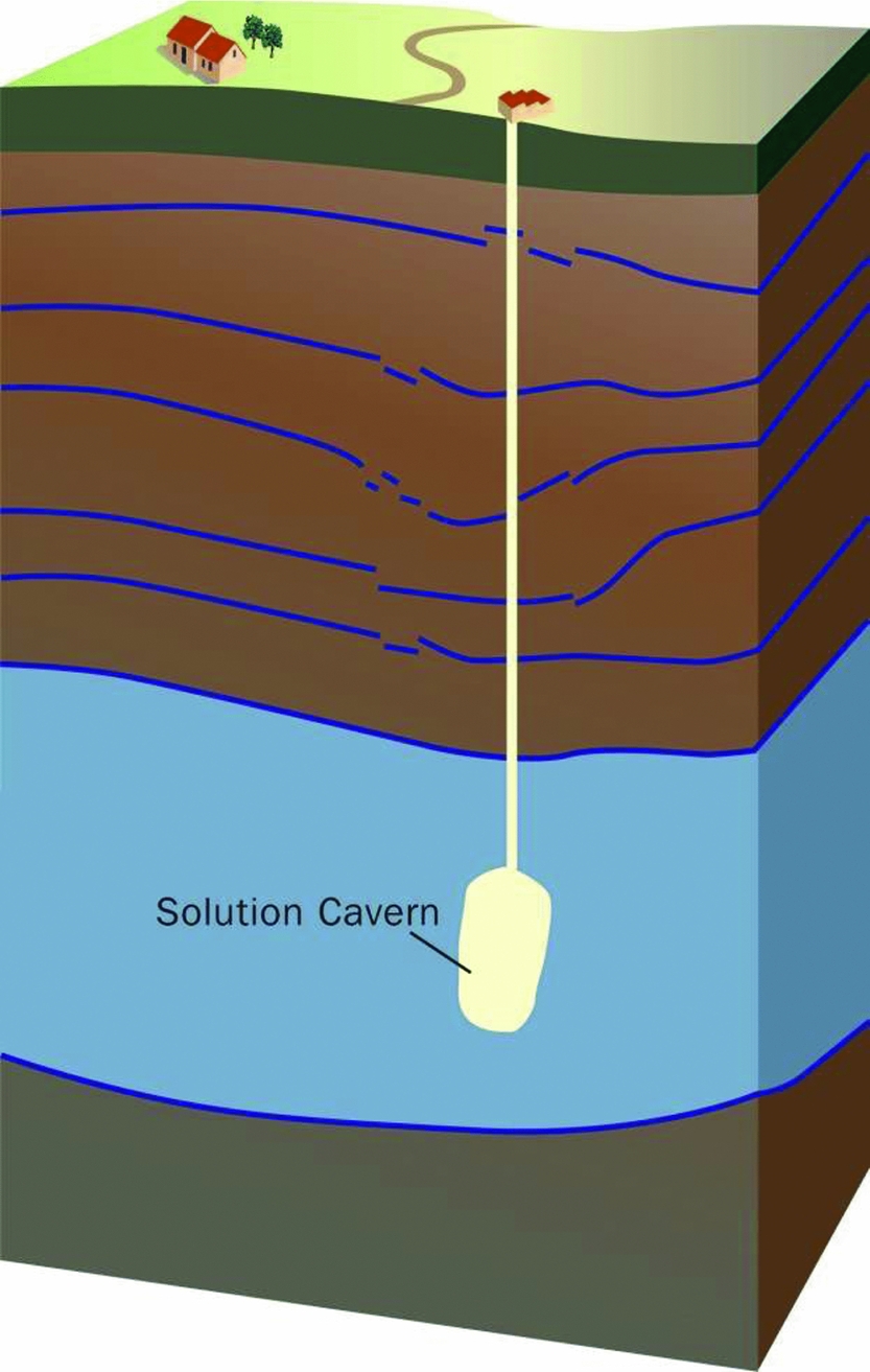
Fig. 4. Underground salt solution cavern (from De Waal et al., Reference De Waal, Roest, Fokker, Kroon, Muntendam-Bos, Oost and van Wirdum2012).
Forward models
Reservoir compaction due to hydrocarbon production and withdrawal of salt from deep geological formations causes changes in the stress field in the subsurface and induces displacement. Forward models used for forecasting ground deformation associated with fluid (oil, gas) or mass (rock salt) extraction from the subsurface are based on analytical and numerical methods. In this section we provide a brief review of forward models for subsidence prediction commonly used in the oil and gas industry and the salt solution mining industry relevant for the Wadden Sea.
Subsidence due to hydrocarbon extraction
The main driver for subsidence associated with hydrocarbon production is decline in the pore fluid pressure in the producing reservoir and connected aquifers, causing compaction of the reservoir and the aquifer. A considerable degree of subsidence requires a considerable degree of reservoir compaction. This can occur when the pressure drop is significant (typically hundreds of bars), the reservoir rock is compressible and the reservoir has a considerable thickness.
Besides a degree of reservoir compaction, it is important how stress changes and deformation propagate outside of a compacting reservoir, towards the ground surface. That will depend on depth, size and structure of the reservoir, as well as on the characteristics of the overburden, its mechanical stratigraphy, the contrast in elastic properties between different formations and possible presence of viscoelastic formations such as the rock salt.
Analytical and semi-analytical methods
Modelling of reservoir compaction and subsidence due to fluid extraction in the oil and gas industry is often done using analytical methods. Analytical approaches typically assume that the reservoir compaction occurs only in the vertical direction and displacements around the compacting reservoir propagate according to some influence function.
Reservoir compaction
Reservoir compaction in a simple basic case can be calculated assuming linear poroelasticity. The compaction is calculated assuming that the lateral extent of a compacting reservoir is much larger than its thickness; in this case the lateral strain can be neglected and the reservoir will compact only uniaxially in the vertical direction (Fig. 5). The reservoir compaction resulting from a certain pore pressure depletion can be estimated as follows (Fjaer et al., Reference Fjaer, Holt, Horsrud, Raaen and Risnes2008):
 $$\begin{equation}
\frac{{\Delta h}}{h} = {C_{\rm{m}}}{\rm{\ }}\alpha {\rm{\ \Delta }}{p_{\rm{f}}}
\end{equation}$$
$$\begin{equation}
\frac{{\Delta h}}{h} = {C_{\rm{m}}}{\rm{\ }}\alpha {\rm{\ \Delta }}{p_{\rm{f}}}
\end{equation}$$
where Δh/h is the vertical strain (i.e. the change in reservoir thickness, Δh, divided by the reservoir thickness, h), α is the Biot's poroelastic coefficient, C m is the uniaxial compaction coefficient or uniaxial compressibility of the reservoir rock, and Δp f is the change in pore fluid pressure. This approach assumes a one-way coupling, i.e. the influence of the compaction on pressure is assumed negligible. C m is related to the intrinsic properties of the reservoir rock: elastic (Young) modulus, E, and the Poisson coefficient, ν:
 $$\begin{equation}
{C_{\rm{m}}} = {\rm{\ }}\frac{{\left( {1 + v} \right)\left( {1 - 2v} \right)}}{{E{\rm{\ }}\left( {1 - v} \right)}}
\end{equation}$$
$$\begin{equation}
{C_{\rm{m}}} = {\rm{\ }}\frac{{\left( {1 + v} \right)\left( {1 - 2v} \right)}}{{E{\rm{\ }}\left( {1 - v} \right)}}
\end{equation}$$
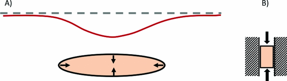
Fig. 5. (A) Schematic representation of a compacting reservoir and related subsidence. Ellipse: compacting reservoir. Dashed line: original ground level. Red line: subsided ground level (B) uniaxial compaction of the reservoir.
The knowledge of parameters required to calculate reservoir compaction generally improves during the production time of the reservoir. The reservoir thickness, h, is usually well constrained from the seismic interpretation and well data. The elastic parameters and α can be measured experimentally on core; however the values of C m determined in the laboratory are often higher (by a factor of 2 and more) than the C m values obtained by inversion of observed subsidence data (NAM, 2016c). Furthermore, the C m values are often spatially variable; for example in sandstone reservoirs they tend to be positively correlated with the porosity.
The change in pore pressure, Δp f, is predicted by a reservoir simulation model calibrated with the available field data. The predictive ability of a reservoir model will be generally lower prior to production, or in the initial phase of production, when the field data are scarce, and will improve towards the mature phase of production, when the simulation model can be history-matched to the observed field data. Possible depletion of connected aquifers can usually be inferred in the mature phase of field production. As a result, the accuracy of predicting reservoir compaction resulting from pressure depletion generally improves during the lifetime of a field.
Different types of compaction models can be used for subsidence calculations. We will describe the linear, the bilinear, the rate type compaction and the time decay model. The linear elastic model is most frequently used in the oil and gas industry. The first two models assume a linear relationship between pressure depletion and compaction. The latter two models introduce a time delay between pressure depletion and compaction in order to better represent the time-dependent subsidence and subsidence-depletion delay from field observations (e.g. Hettema et al., Reference Hettema, Papamichos and Schutjens2002).
• The linear elastic compaction model assumes a constant value for the compaction coefficient C m of the reservoir rock during the whole depletion period. The C m value can spatially vary over the reservoir, for example as a function of porosity.
• The bilinear elastic model assumes two values for the compaction coefficient C m in an attempt to better match field observations of the temporal subsidence behaviour above depleting gas fields: a slow subsidence rate in the first years of production followed by a faster subsidence rate afterwards. Accordingly, the C m value for the initially stiff, less compressible reservoir rock is changed at transition depletion pressure to the Cm value for the less stiff, more compressible reservoir rock. The rationale for using a bilinear model is borrowed from the soil mechanics and is likely plausible for application to overpressurised gas reservoirs (reservoirs with the initial pressure above hydrostatic) which are assumed less compressible until the reservoir pressure has decreased to the hydrostatic pressure level (e.g. Hettema et al., Reference Hettema, Papamichos and Schutjens2002).
• The rate type compaction model (RTCM) assumes that the compaction behaviour is dependent on the loading rate (de Waal, Reference De Waal1986). Recently, the RTCM was combined with the isotach model used to describe deformational behaviour of soft soils in geotechnics (Pruiksma et al., Reference Pruiksma, Breunese, van Thienen-Visser and de Waal2015). The new isotach formulation of the RTCM describes in a consistent way the compaction behaviour of sandstone for changes in loading rates, including the transition to a constant load essential to describe creep. The model gives excellent agreement with laboratory tests and still needs to be tested in field conditions.
• The time-decay compaction model introduces a delayed response of reservoir compaction to pressure depletion (Mossop, Reference Mossop2012). A time lag can be calculated from the diffusion equation, assuming an exponential time-decay function and determining the value of a time-decay constant by fitting the modelled to the observed subsidence. A diffusive time-decay process is here used as a concept to explain a delay in the onset of compaction and subsidence; however, this approach lacks real physical processes responsible for delay.
The relationship between compaction and subsidence
Deformation of the compacting reservoir propagates through the overburden and causes surface subsidence. Compaction at reservoir level and surface subsidence are mutually dependent. Most of the methods for calculation of subsidence due to fluid extraction used in the oil and gas industry are based on the ‘nucleus of strain’ concept described by Geertsma (Reference Geertsma1973a,b). Geertsma's solution is physically based and follows the concept of nucleus of strain introduced by Mindlin (Reference Mindlin1936) and Mindlin & Cheng (Reference Mindlin and Cheng1950) in the theory of thermoelectricity. In Geertsma's model, the subsurface is represented by a homogeneous, isotropic, linear-elastic half-space. The compacting reservoir is represented by many small, compacting spheres (centre of compression). The displacements are calculated for each sphere using a Green's function. Finally, the influence of all spheres is summed up to obtain the total subsidence in a domain of interest.
The basic formulation for subsidence from a nucleus of strain is given by the following expressions:
 $$\begin{equation}
{U_z}{\rm{\ }}\left( {r,0} \right) & =& - \frac{1}{\pi }{C_{\rm{m}}}{\rm{ }}\left( {1 - v} \right){\rm{ }}\frac{D}{{{{({r^{2{\rm{ }}}} + {\rm{ }}{D^{2{\rm{ }}}})}^{\frac{3}{2}}}}}{\rm{ }}\alpha \pi {R^2}{\rm{ }}H{\rm{\ \Delta }}{p_{\rm{p}}}\quad\\
\end{equation}$$
$$\begin{equation}
{U_z}{\rm{\ }}\left( {r,0} \right) & =& - \frac{1}{\pi }{C_{\rm{m}}}{\rm{ }}\left( {1 - v} \right){\rm{ }}\frac{D}{{{{({r^{2{\rm{ }}}} + {\rm{ }}{D^{2{\rm{ }}}})}^{\frac{3}{2}}}}}{\rm{ }}\alpha \pi {R^2}{\rm{ }}H{\rm{\ \Delta }}{p_{\rm{p}}}\quad\\
\end{equation}$$
 $$\begin{equation}
{U_{\rm{r}}}{\rm{ }}\left( {r,0} \right) & =& - \frac{1}{\pi }{C_{\rm{m}}}{\rm{ }}\left( {1 - v} \right){\rm{ }}\frac{r}{{{{({r^{2{\rm{ }}}} + {\rm{\ }}{D^{2{\rm{ }}}})}^{\frac{3}{2}}}}}{\rm{ }}\alpha \pi {R^2}{\rm{\ }}H{\rm{ \Delta }}{p_{\rm{p}}}\quad
\end{equation}$$
$$\begin{equation}
{U_{\rm{r}}}{\rm{ }}\left( {r,0} \right) & =& - \frac{1}{\pi }{C_{\rm{m}}}{\rm{ }}\left( {1 - v} \right){\rm{ }}\frac{r}{{{{({r^{2{\rm{ }}}} + {\rm{\ }}{D^{2{\rm{ }}}})}^{\frac{3}{2}}}}}{\rm{ }}\alpha \pi {R^2}{\rm{\ }}H{\rm{ \Delta }}{p_{\rm{p}}}\quad
\end{equation}$$
Fig. 6A plots the amount of normalised subsidence (Uz/ΔH) as a function of normalised distance from the centre of a disc-shaped reservoir (r/R). Apparently, subsidence is concentrated directly above the centre of a depleting reservoir. For a reservoir of a certain radial extent, the amount of maximum subsidence above it can range from ~0.8 down to 0.05 times the total compaction when the depth increases from 0.2 to 3.0 times the radial extent (Fig. 6A). Fig. 6B plots the amount of normalised horizontal radial displacement (U r/ΔH) as a function of normalised distance from the centre of the reservoir. The amount of maximum horizontal displacement is 2.5–3 times smaller than the amount of maximum subsidence. The horizontal displacement is concentrated above the boundary of the reservoir.
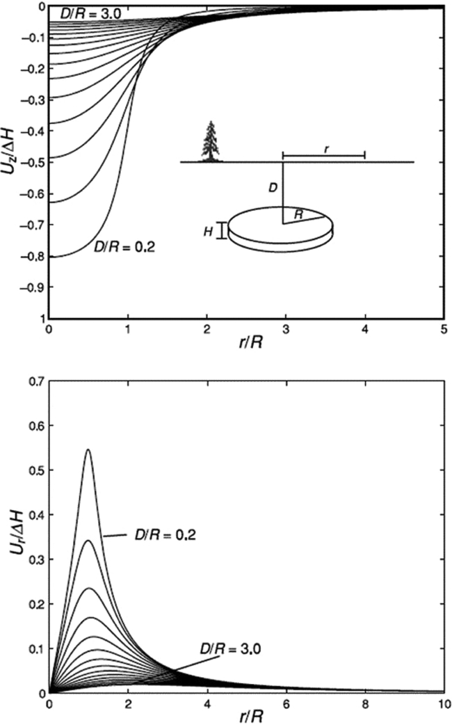
Fig. 6. Normalised (top) subsidence Uz and (bottom) horizontal displacement Ur above a disc-shaped compacting reservoir of radius R and initial thickness H, at depth D. The reservoir compacts ΔH following the analytical solution of Geertsma (Reference Geertsma1973a,b). Maximum subsidence occurs above the centre of the reservoir, and maximum horizontal displacement occurs at the reservoir edge. (From Zoback, Reference Zoback2007, p. 414.)
The initial Geertsma's model was later further developed by others. Van Opstal (Reference Van Opstal1974) studied the vertical displacement at the free surface, adding a rigid basement to Geertsma's model. Fares & Li (Reference Fares and Li1988) presented a general image method for a plane-layered elastic medium, which involves infinite series of images. Fokker & Orlic (Reference Fokker and Orlic2006) proposed a semi-analytical model for the calculation of subsidence in a multi-layered viscoelastic subsurface (Fig. 7). This semi-analytical model satisfies the elasticity equations by combining a number of analytic functions in such a way as to approximate boundary conditions at layer interfaces. The thickness of model layers needs to be larger than ~0.1 of the reservoir depth for a reliable model prediction.
Fig. 7. Schematisation of a producing hydrocarbon reservoir, embedded in a multi-layered elastic subsurface, for subsidence calculations by the semi-analytical method developed by Fokker & Orlic (Reference Fokker and Orlic2006).
Another approach for estimating subsidence, mainly used in the mining industry, is based on the concept of an influence function. Knothe's influence function (Knothe, Reference Knothe1953), originally developed for subsidence prediction due to coal mining in Central Europe, is one of the most popular. Knothe adopted the influence function, F, based on a Gaussian function:
 $$\begin{equation}
F{\rm{\ }} = {\rm{\ }}\frac{1}{{{R^2}}}\exp \left( { - \pi \ \frac{{{d^2}}}{{{R^{2\ }}}}} \right)
\end{equation}$$
$$\begin{equation}
F{\rm{\ }} = {\rm{\ }}\frac{1}{{{R^2}}}\exp \left( { - \pi \ \frac{{{d^2}}}{{{R^{2\ }}}}} \right)
\end{equation}$$
where R is the radius of influence defined as R=Dtan(φ), D is the reservoir depth and φ is the influence angle. The Knothe theory was later modified by several authors who defined different influence functions that presumably better fitted observed subsidence in a particular mined-out area. Knothe's work was extended to include a time delay between compaction (i.e. mineral extraction in the mining) and subsidence, and also applied in the oil and gas industry for prediction of subsidence due to fluid withdrawal (Hejmanowski, Reference Hejmanowski1993; Hejmanowski & Sroka, Reference Hejmanowski and Sroka2000).
The drawback of using influence functions to predict subsidence from reservoir compaction is that the method is not based on physical processes and it cannot predict horizontal displacement. A possible advantage is that the radius of influence, and consequently the extent of the subsidence bowl, is an input parameter, which could be matched to field observations.
The volume of the subsidence bowl that results from an influence function approach is not necessarily equal to the volume of compaction in the reservoir, while there is still no volume strain outside the compaction zone. This is not physically inconsistent, because the influence functions are based on solutions to the poroelastic equations that are not bounded in space. A vanishingly small displacement very far away from the compacting source can give rise to a finite volume when integrated over an area that extends to infinity (Van Opstal, Reference Van Opstal1974). Van Opstal showed that the volume of the subsidence bowl equals a factor 2(1−ν) (i.e. a factor 1.5 for ν=0.25) times the volume of reservoir compaction for Geertsma's solution (valid for a homogeneous, isotropic, linear-elastic half-space); while the application of a rigid basement results in volume conservation. This was attributed to an effective constraint on the vertical extent of the subsurface.
Numerical methods
A different approach is the use of numerical codes, such as finite elements, for subsidence calculations. A numerical approach enables simulation of the full relationship between flow in the porous medium and induced geomechanical responses (Fig. 8), taking into account complex structural–geological settings and heterogeneity of the subsurface (Settari & Walters, Reference Settari and Walters2001). An additional major advantage is the possibility to describe the mechanical behaviour of geological formations by complex, nonlinear, constitutive laws. In contrast to the analytical models, the field-scale numerical models of the subsurface require significantly more time for construction and computation.
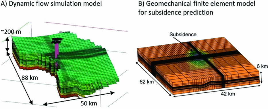
Fig. 8. (A) Reservoir simulation model of the Agostino – Porto Garibaldi gas field in the northern Adriatic, Italy, and (B) a spatially extended geomechanical finite element model for subsidence calculations due to gas extraction from the same field. Geomechanical numerical model comprises gas reservoir, surrounding aquifers and geological formations above and below the reservoir (Schroot et al., Reference Schroot, Fokker, Lutgert, van der Meer, Orlic, Scheffers and Barends2005).
Field-scale numerical models of hydrocarbon fields are employed for the analysis of complex geomechanical phenomena that cannot be predicted in satisfactory manner by analytical modelling and (could) have significant financial or environmental impact. Common examples are: excessive and anomalous subsidence, induced seismicity due to production-induced fault reactivation and well integrity-related issues in complex structural settings.
A numerical approach for the analysis of subsidence due to extraction of gas from a number of fields located in the Northern Adriatic has been successfully employed by ENI in the last decade (Capasso & Mantica, Reference Capasso and Mantica2006; Gemelli et al., Reference Gemelli, Monaco and Mantica2015). Subsidence affects the coastal area of Ravenna, south of Venice. A one-way coupling scheme is used between the reservoir- and the geomechanical simulator. Deformational behaviour of the reservoir rock is described by different constitutive laws that can capture the nonlinearity and time dependence of deformation, e.g. the elasto-plastic Modified Cam Clay model and the elasto-viscoplastic Vermeer and Neher constitutive law (Nguyen et al., Reference Nguyen, Volonté, Musso, Brignoli, Gemelli and Mantica2016). Field-scale subsidence models are regularly updated and calibrated with subsidence data. Another example of using field-scale numerical models to predict accelerating subsidence above highly compacting carbonate reservoirs, offshore Sarawak Malaysia, was reported by Khalmanova & Dudley (Reference Khalmanova and Dudley2008) and Dudley et al. (Reference Dudley, van den Linden and Math2009). In this case the objective was to provide a subsidence prediction for the platform. In the Netherlands, field-scale numerical models of gas fields for subsidence prediction were developed for the Ameland gas field (G. Schreppers, unpublished report, 1998; Marketos et al., Reference Marketos, Broerse, Spiers and Govers2015). The latter study focused on time-dependent subsidence due to induced flow of viscoelastic rock salt above the reservoir.
Besides for subsidence prediction, field-scale geomechanical numerical models of hydrocarbon fields were developed for different applications: for example, to study production-induced seismicity at Groningen gas field (Lele et al., Reference Lele, Hsu, Garzon, DeDontney, Searles, Gist, Sanz, Biediger and Dale2016); to evaluate geomechanical effects of underground gas storage operations on the stability of faults in a gas field in the Netherlands with the previous record of induced seismicity (Orlic et al., Reference Orlic, Wassing and Geel2013); to study production-induced stress changes in a mechanically complex high-pressure high-temperature (HPHT) field for field development and infill drilling (De Gennaro et al., Reference De Gennaro, Schutjens, Fruman, Fuery, Ita and Fokker2010); to analyse wellbore integrity for infill wells in structurally complex fields with highly compressible reservoirs and faults prone to reactivation (e.g. Shearwater field in the North Sea, Kenter et al., Reference Kenter, Blanton and Schreppers2008); and to study production-induced stresses in and around reservoirs close to salt domes (Schutjens et al., Reference Schutjens, Snippe, Mahani, Turner, Ita and Mossop2010).
Subsidence due to salt solution mining
We consider subsidence due to deep solution salt mining such as in the Barradeel concessions in Friesland, the Netherlands, at a depth of 2.5–3km, which is among the deepest in the world. Similar salt solution mining is also planned from under the Wadden Sea in Havenmond from 2018 as discussed in the section ‘Salt solution mining in Havenmond’ below. The shape of solution mined caverns in Barradeel is roughly cylindrical, with a radius of 20–30m and a height of 300–400m. As mentioned in the previous section, after a few years of leaching, the steady-state conditions are usually reached; from that time on, volume and shape of a cavern stay approximately constant during further production, which makes subsidence prediction generally somewhat easier. The shape and volume of a cavern can be measured by sonar surveys.
Both analytical and numerical approaches are used to calculate subsidence due to salt solution mining. Analytical approaches are based on the use of influence functions which relate the converged salt volumes and surface subsidence. The convergence volume is the difference between the volumes of produced salt and of the cavern. Two assumptions are usually made (L.L. van Sambeek, unpublished observations, 2016): (i) total subsidence volume cannot exceed the cumulative closure volume of the cavern; and (ii) incremental (annual) change in subsidence volume is equal to a change in cavern volume (Fig. 9). The assumptions used in the salt-solution mining to derive influence functions for subsidence calculations are pragmatic and intuitive, but different from those used in Geertsma's and Van Opstal's solutions where the volume of the subsidence bowl is not necessarily equal to the volume of reservoir compaction or salt squeeze (see ‘Analytical and semi-analytical methods’ above). Further, an assumption is made about the area affected by subsidence by specifying the angle of draw, usually 45°. The shape of the subsidence bowl is usually assumed Gaussian.
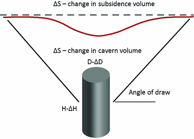
Fig. 9. Schematic representation of a salt cavern and subsidence due to salt extraction used to illustrate the main principle applied in analytical methods for subsidence calculations. The changes in cavern diameter (from D to D−ΔD) and height (from H to H−ΔH) cause a change in volume ΔS of the cavern and an identical volume of the subsidence bowl.
Gaussian shape is also a good approximation of the measured subsidence in the Barradeel concession (Fokker et al., Reference Fokker, Bakker, Wilke and Barge2002; T.W. Bakker & A.J.H. Duquesnoy, unpublished report, 2010). The shape of the subsidence bowl can be determined by using
 $$\begin{equation}
Z\left( r \right){\rm{\ }} = {Z_{{\rm{max}}}}{\rm{exp\ }}\left( { - \gamma {\rm{\ }}{r^\delta }} \right) = {\rm{\ }}\chi {\rm{\ }}{V_{{\rm{con}}}}{\rm{\ exp\ }}\left( { - \gamma {\rm{\ }}{r^\delta }} \right)
\end{equation}$$
$$\begin{equation}
Z\left( r \right){\rm{\ }} = {Z_{{\rm{max}}}}{\rm{exp\ }}\left( { - \gamma {\rm{\ }}{r^\delta }} \right) = {\rm{\ }}\chi {\rm{\ }}{V_{{\rm{con}}}}{\rm{\ exp\ }}\left( { - \gamma {\rm{\ }}{r^\delta }} \right)
\end{equation}$$
where Z(r) is the subsidence at a radial distance r from the centre of the subsidence bowl, Z max is the maximum subsidence in the centre of the subsidence bowl, γ is a dimensionless parameter which determines the radial extent of the bowl, δ is a dimensionless parameter which determines the slope of the flanks of the bowl, χ is a scale factor to determine the relationship between the subsidence rate in the centre of the subsidence bowl and the converged salt volume, and V con is the volume of produced salt, which equals the volume of converged salt. In practice, the model parameters are determined by calibration to measured subsidence data.
The described analytical approach and eqn 6 are generally valid for the steady-state phase of salt squeeze when volume and shape of the cavern stay approximately constant (see the previous section), but not for the initial phase of cavern leaching when the cavern grows in size, and the post-abandonment phase, when the shape of the subsidence bowl can still change over time due to salt viscosity. Instead, numerical approaches are required as discussed below.
An analytical model based on material balance was developed by Breunese et al. (Reference Breunese, van Eijs, de Meer and Kroon2003). This data-driven material balance model describes the time evolution of the cavern volumes, the cavern volume convergence rate and the maximum subsidence at the centre of the subsidence bowl. The model was developed and successfully used to predict the maximum subsidence above the deep solution salt caverns in the Barradeel concessions in the Netherlands.
Numerical, solid-physics models are widely used to study stability and integrity of caverns and subsidence. The major advantage of using numerical models (compared to analytical models) is the ability to model the highly nonlinear, time-dependent process of creep in the rock salt, which is the main deformational mechanism causing salt squeeze, cavern convergence and surface subsidence. Different constitutive laws exist and are implemented in different numerical codes. Finite element models of caverns in the Barradeel concession were constructed and successfully applied to predict the evolution of surface subsidence caused by salt solution mining from two deep caverns located at a depth of 2.5–3km (Breunese et al., Reference Breunese, van Eijs, de Meer and Kroon2003).
The study focused mainly on the prediction of maximum subsidence. The creep of salt was modelled using a combination of a linear and a power-law creep model for the secondary, steady-state creep (Fokker, Reference Fokker1995) to be able to match the subsidence measurements. Results showed that the ratio of maximum subsidence (at the centre of the subsidence bowl) and the converged salt volume was not constant over time due to simultaneous action of two deformational mechanisms in salt: (i) the dislocation creep (represented by a nonlinear creep model), which accelerates subsidence and (ii) the pressure solution creep (represented by a linear creep model), which decelerates subsidence. Further, the shape of the subsidence bowl also changes over time, generally from a deeper and narrower bowl during the steady-state phase of salt leaching to a shallower and wider bowl, which develops after the cessation of salt production and cavern abandonment.
Although the numerical approach is conceptually better than the analytical approach, construction of meshes and numerical computations require much more time, which is why the analytical approach is much more often used for subsidence calculations in the salt-solution mining industry.
Measuring subsidence
Surface motion measurements vs the signal of interest
Surface subsidence (or heave) is defined as a relative height change over time between two locations or points. It can be measured using techniques which are inherently relative, such as levelling or InSAR, or using techniques which provide positions in a geodetic datum (reference system), such as Global Navigation Satellite Systems (GNSS). For the latter category, it needs to be assumed that the geodetic datum is time-independent.
There are various techniques to measure heights, (spatial) height differences, (temporal) height change, or (spatio-temporal) changes in height differences. These techniques can be spaceborne, airborne or terrestrial, and have their own characteristics regarding spatial density of measurements, spatial extent, temporal sampling frequency, temporal extent, geometric sensitivity, and precision. An overview of the most important height measurement techniques and their characteristics is given in Table 1.
Table 1. Overview of height change measurement techniques and their typical characteristics.
As shown in Table 1, the spatial density and temporal sampling frequency differ greatly between the various measurement techniques. Some techniques require pre-installed man-made benchmarks, others are more opportunistic and use natural points which require no preparation. Some techniques measure heights onshore, while others operate offshore (i.e. the bathymetry of the sea floor or markers under water). Moreover, the sensitivity of the measurement may be different. GNSS are actually measuring 3D positions. In case of satellite radar interferometry (InSAR), the measurements are taken in the radar line-of-sight between the satellite and the surface.
Hereby, the measurements are sensitive to both vertical and horizontal motion. Also, the type of height parameter is different for the various techniques. In case of levelling, orthometric height differences are obtained, i.e. height differences in the direction parallel to the local gravity acceleration vector. These height differences have a physical meaning. This also holds for gravimetric height differences. For the other techniques the height differences are defined geometrically, in a reference frame of choice. For local subsidence, and if the changes in mass distribution over time can be ignored, the difference between different height definitions is negligible.
For some techniques, dedicated benchmarks or receivers are required. This has the advantage that exactly the same points are measured over time and the subsidence can be estimated directly from the repeated height difference measurement. In other cases, the measurements are based on natural reflection points of the optical or radio signals. For laser altimetry and echo sounding measurements this will result in a distribution of measurement points that is different at each epoch or survey. As a result, subsidence estimation cannot be performed point-wise, requiring a form of collocation of the points, e.g. by interpolation. For InSAR, however, these reflection point positions are consistent over time, so no interpolation is needed and subsidence can be directly estimated from the repeated height difference measurements.
Irrespective of the type of measurement points used, the sensitivity of the measurements for the motion of a certain layer in the (sub)surface depends on the mechanical foundation of the benchmark or reflection point. An illustration is given in Fig. 10 for the case of benchmarks in buildings (Ketelaar, Reference Ketelaar2009). The total measured subsidence at the surface is the sum of all compaction processes in the subsurface. However, not all benchmarks will be sensitive to all compaction effects. Moreover, local instability of foundations will result in anomalous behaviour, often denoted as ‘autonomous movement’ of the point involved. For a proper interpretation of the estimated subsidence, the impact of the different foundations should be taken into account. This not only holds for the techniques using benchmarks, but also for the natural reflection points (see section ‘InSAR/PSI’ below).
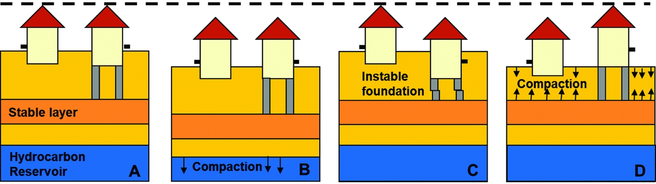
Fig. 10. The effect of different causes on the measured surface subsidence in case benchmarks are used. (A) Original situation, with a benchmark (in black) in a building with deep foundation on a stable layer, or in a building without foundation. (B) In case of compaction of a hydrocarbon reservoir, measurement of both benchmarks will result in the same surface motion. (C) In case of an instable foundation, a local subsidence signal would be measured, whereas no compaction occurs. (D) In case of shallow compaction, only a subsidence signal will be measured at the unfounded benchmark.
Hence, depending on the objective, different subsidence regimes should be separated. We refer to the degree to which the measurements represent the actual signal of interest as the idealisation accuracy. It should be noted that the idealisation accuracy is completely unrelated to the measurement precision.
In practice, for subsidence analysis, typically levelling, GNSS and/or InSAR measurements are used. This is related to their spatial and temporal sampling density and extent, measurement precision, and cost. Up to now, the number of laser altimetry measurement epochs is low, and their precision and reliability for changes in height differences is low, which is why these measurements are not incorporated. The precision of echo sounding measurements (and the associated platform positioning) is in general too low for detecting relatively low subsidence rates. These measurements are therefore more often used for morphological changes in the sea floor. The use of in situ sensors, such as extensometers, is limited to local applications with limited spatial extent. Finally, the number of (absolute and relative) gravity stations is typically limited, and surveys are expensive and difficult. Therefore, further focus in this section will be given to the conventional techniques: optical levelling, hydrostatic levelling, GNSS and InSAR.
Optical levelling
With optical levelling, relative height differences are measured between fixed benchmarks. These benchmarks are either part of a national height reference framework, or can be a densification thereof, installed for a particular application. In the Netherlands, the national height reference network is physically represented by about 360 subsurface benchmarks anchored in the Pleistocene stratum, up to 25m below the surface. This includes 67 special Pleistocene benchmarks close to tide gauge stations along the main rivers, the Noordzee and the Wadden Sea (De Bruijne et al., Reference De Bruijne, van Buren, Kösters and van der Marel2005). This primary network is densified by about 35,000 secondary benchmarks. As a result, in general, on land a reference benchmark can be found within 1km, anywhere in the Netherlands.
The main purpose of this dense set of benchmarks is to be able to estimate the height of arbitrary objects or structures by performing a simple and relatively short levelling between the object and a nearby reference benchmark. For this pragmatic purpose, it is assumed that the height of the reference benchmarks does not change over time. This hypothesis is checked by a levelling campaign typically every 10 years for the secondary benchmarks. In the meantime, even if the benchmark subsides, this will not be noticed. The levelling campaign relates the secondary benchmarks to the primary (subsurface) benchmarks, which are also assumed to be stable over time. Campaigns to verify this hypothesis are performed typically every 25– 30 years, and in the meantime, motion of the network would not be detected. As such, the entire set-up of the set of reference benchmarks is not tuned to detect or monitor vertical land motion.
Although single epoch height values of the physical benchmarks are meaningless in relation to subsidence, the most recent estimated height value is made available via the PDOK website (see http://pdokviewer.pdok.nl/). An archive of the historic height values of the benchmarks is potentially useful for subsidence monitoring, considering the link with the presumably stable primary benchmarks. Levelling measurements are archived by Rijkswaterstaat (see ‘Data availability in the Wadden Sea region’ below).
Levelling measurements are performed in networks with closed loops, to allow for the adjustment and testing of the observations. A generic approximation for the standard deviation σ ol (mm) of the optical levelling measurements is
 $$\begin{equation}
{\sigma _{{\rm{ol}}}}{\rm{\ }} = {\rm{\ }}{{\rm{c}}_0}{\rm{\ }} + {\rm{\ }}{{\rm{c}}_1} \cdot \sqrt l
\end{equation}$$
$$\begin{equation}
{\sigma _{{\rm{ol}}}}{\rm{\ }} = {\rm{\ }}{{\rm{c}}_0}{\rm{\ }} + {\rm{\ }}{{\rm{c}}_1} \cdot \sqrt l
\end{equation}$$
where l is the length of the levelling trajectory in km. Typical values for c 0 are within 0 and 2mm (Hanssen et al., Reference Hanssen, Kremers, van der Marel, Barends, Dillingh, Hanssen and van Onselen2008), whereas values between 0.64 and 1.29mm/√km hold for c 1 (Leusink, Reference Leusink2003). Based on the adjustment results of the fifth precision levelling of the primary benchmarks (5e Nauwkeurigheidswaterpassing) of the Netherlands, Brand (Reference Brand2004) came to a relative precision (mm) of adjusted heights of
 $$\begin{equation}
{\sigma _{{\rm{ol}},{\rm{rel}}}}{\rm{\ }} = {\rm{\ }}2 + 0.2 \cdot \sqrt l
\end{equation}$$
$$\begin{equation}
{\sigma _{{\rm{ol}},{\rm{rel}}}}{\rm{\ }} = {\rm{\ }}2 + 0.2 \cdot \sqrt l
\end{equation}$$
Hydrostatic levelling
Hydrostatic levelling is based on the principle of communicating vessels. The water level at both ends of a long tube is used to transfer a height. The tubes are laid in water bodies, and therefore the trajectories of hydrostatic levelling campaigns follow rivers and coastlines. In the Netherlands, hydrostatic measurements were performed by Rijkswaterstaat, using a dedicated ship. Tubes of different lengths were available, which could be connected to reach a maximum length of 12km. Due to the ageing of the ship, changes in the occupational safety rules, and the emergence of GNSS for height measurements, the ship was taken out of operation in 2003 (Kösters, Reference Kösters2001). As a result, hydrostatic measurements are no longer performed in the Netherlands (an additional hydrostatic levelling was performed in 2005, between Harlingen and the Zuidwal platform, using an existing glycol tube connection (source: nlog.nl)) and are replaced by GNSS measurements (Brand & Ten Damme, Reference Brand and Ten Damme2004). Nevertheless, the historic hydrostatic levelling measurements are still relevant for deformation analysis.
For hydrostatic levelling measurements, in practice the tolerance V (mm) was used to set the allowed deviation in the difference between the mean of both a set of forward and a set of backward hydrostatic levelling measurements (Van Vliet et al., unknown). Typically, a set of five measurements was used in both directions. The tolerance is dependent on the length of the tube L (in km) used, and is set by
 $$\begin{equation}
V = 0.8 + 0.1 \cdot L
\end{equation}$$
$$\begin{equation}
V = 0.8 + 0.1 \cdot L
\end{equation}$$
Assuming this tolerance can be translated to a 95% confidence interval, the tolerance can also be expressed as a function of the standard deviation σ m of a one-way mean hydrostatic levelling as
 $$\begin{equation}
V = {\rm{\ }}1.96{\sigma _{\rm{m}}}\sqrt 2
\end{equation}$$
$$\begin{equation}
V = {\rm{\ }}1.96{\sigma _{\rm{m}}}\sqrt 2
\end{equation}$$
0where √2 accounts for the difference between the forward and backward levelling.
Hence, the standard deviation of a mean hydrostatic levelling reads
 $$\begin{equation}
{\sigma _{\rm{m}}} = \frac{V}{{1.96\sqrt 2 }}
\end{equation}$$
$$\begin{equation}
{\sigma _{\rm{m}}} = \frac{V}{{1.96\sqrt 2 }}
\end{equation}$$
The standard deviation σ mm of the mean of a mean forward and a mean backward hydrostatic levelling is therefore
 $$\begin{equation}
{\sigma _{{\rm{mm}}}} = \frac{V}{{1.96{\rm{\ }}\sqrt 2 {\rm{\ }}\sqrt 2 }} \approx \frac{1}{4}V
\end{equation}$$
$$\begin{equation}
{\sigma _{{\rm{mm}}}} = \frac{V}{{1.96{\rm{\ }}\sqrt 2 {\rm{\ }}\sqrt 2 }} \approx \frac{1}{4}V
\end{equation}$$
The associated values are summarised in Table 2. Hence, the precision of a single hydrostatic levelling is in the order of 0.25–0.50mm.
Table 2. Tolerances and associated standard deviations of hydrostatic levelling as a function of tube length (Van Vliet et al., unknown).
A number of corrections must be applied to the hydrostatic measurements, to account for (i) capillary action, (ii) temperature differences, (iii) air pressure differences and (iv) tidal effects due to the sun and the moon (Van Vliet et al., unknown). Since the hydrostatic levelling measurements cannot be connected directly to fixed benchmarks, short optical levelling measurements are performed to make the connection. Once connected, an adjustment and testing procedure is applied, possibly in combination with the optical levelling measurements, to estimate the heights and to detect outliers in the data.
GNSS
The Global Positioning System (GPS) has found widespread use in civilian navigation, land and hydrographic surveying, high-precision positioning and navigation, deformation monitoring, meteorology and a host of scientific applications (Teunissen and Kleusberg, Reference Teunissen and Kleusberg1998; Bock & Melgar, Reference Bock and Melgar2016). GPS is one class of GNSS; other systems are the Russian Glonass system, the European Galileo system and the Chinese Beidou system. All of these systems provide functionality similar to GPS, and if combined, extend beyond the capabilities of a single system (Teunissen & Montenbruck, Reference Teunissen and Montenbruck2017). GNSS satellites broadcast a time code, and the GNSS receiver compares the broadcasted time code with a clock inside the receiver. The difference, when multiplied by the speed of light, is the so-called pseudo-range measurement. Ignoring satellite and receiver clock errors, atmospheric delays and measurement error, the pseudo-range measurement is equal to the distance between satellite and receiver (see Fig. 11). If a minimum of four satellites are tracked, the GNSS receiver can estimate its position in the WGS-84 reference system (Hofmann-Wellenhof et al., Reference Hofmann-Wellenhof, Legat and Wieser2003; Seeber, Reference Seeber2003; Misra & Enge, Reference Misra and Enge2006).
Fig. 11. GNSS measurement principle (from Misra & Enge, Reference Misra and Enge2006).
The typical accuracy that can be obtained by GPS is 1–2m horizontally and 3–5m vertically. This accuracy is not sufficient for surveying and deformation monitoring. However, geodetic GPS receivers in combination with specialised post-processing procedures enable centimetre to millimetre accuracies over baselines reaching from a few kilometres up to several thousands of kilometres (Teunissen & Kleusberg, Reference Teunissen and Kleusberg1998). Fig. 12 gives a couple of examples of modern geodetic GNSS receivers. What sets a geodetic receiver apart from mass-market receivers is its ability to track the carrier phase. This provides millimetric range measurement to the GNSS satellites, albeit with a constant time ambiguity of a multiple of integer wavelengths. Furthermore, a geodetic receiver can track multiple frequency bands. GNSS satellites broadcast at different frequency bands (common bands are known as L1, L2 and L5). Tracking two or three of these bands allows for the elimination of ionospheric delays in the processing.
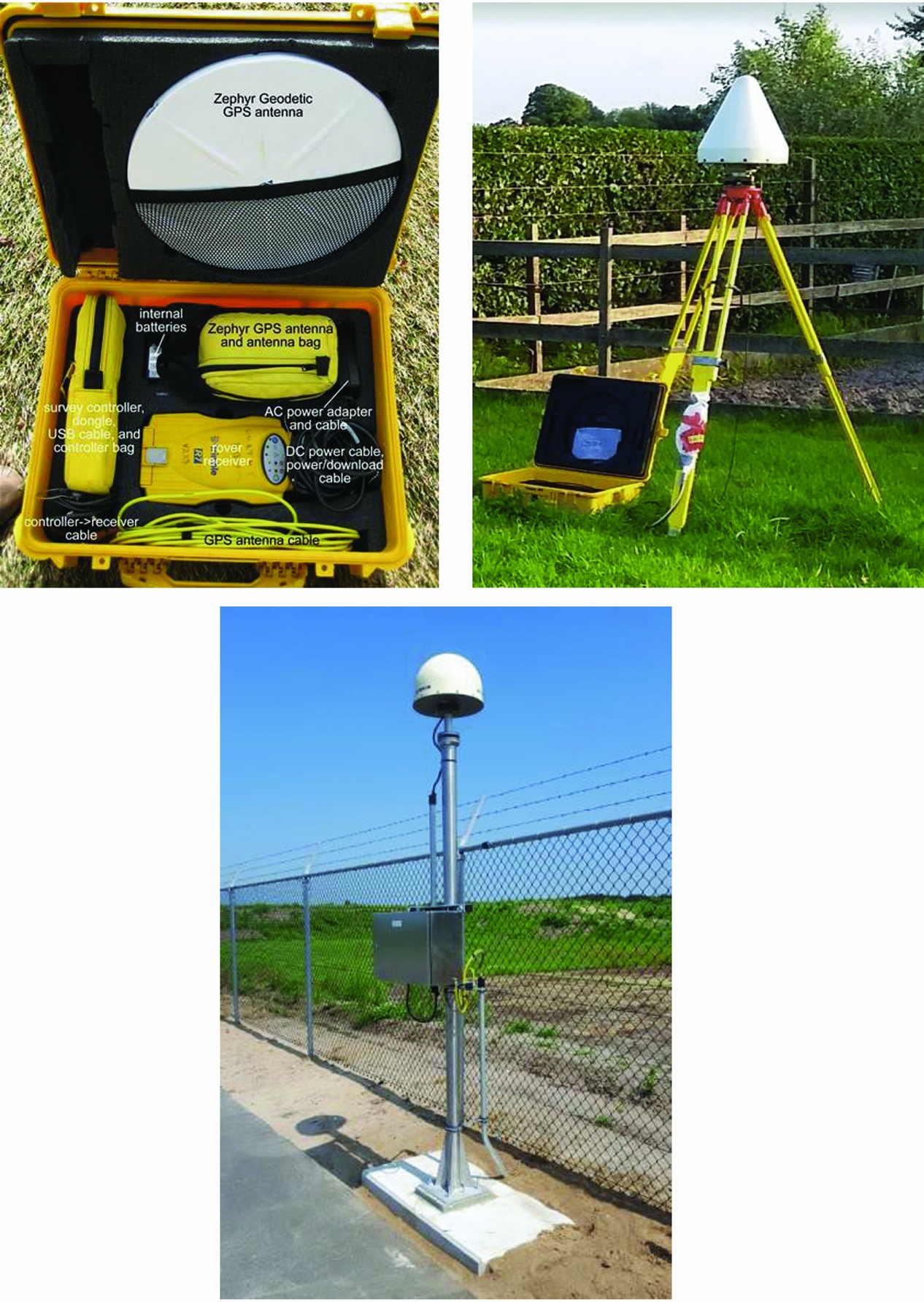
Fig. 12. Three examples of a geodetic receiver unit. On the left a campaign receiver and antenna in a case with all accessories (image courtesy UNAVCO), in the middle a typical field set-up with antenna on a tripod centred above a marker and battery-powered receiver in the waterproof case (data are stored on a flash card inside the receiver) (image TU Delft), and on the right a Continuous Operating Reference Station (CORS) from NAM, with receiver and data modem inside the cabinet (image courtesy 06-GPS).
Carrier phase measurements are key to high-precision positioning and navigation. The carrier phase measurement has an accuracy of 1–2mm, but it is ambiguous in the integer number of wavelengths. Special processing techniques are necessary to solve for these ambiguities, but once these are solved, millimetre-level relative position accuracies can be obtained.
The high-precision positioning technique is essentially a relative technique, similar to levelling or InSAR. It involves two receivers. The reference receiver is installed on a benchmark with coordinates assumed known (base station); for the rover receiver the coordinates will be computed. The distance between the receivers may vary, but it is useful to distinguish between short baselines up to 10–20km, and long baselines up to several hundreds of kilometres. For short baselines, the effects of satellite ephemerides errors are strongly reduced (satellite position) or completely eliminated (satellite clock). Also the effect of atmospheric errors is strongly reduced as these are very similar at both ends of the baseline. The relative precision of the baseline vector varies between several mm and a few cm, depending on the distance and a few other factors. The precision in the height component is always worse than the precision of the horizontal components (Hofmann-Wellenhof et al., Reference Hofmann-Wellenhof, Legat and Wieser2003; Misra & Enge, Reference Misra and Enge2006). For longer baselines centimetre accuracy is possible, provided that (i) multi-frequency data are used to eliminate ionospheric delays, (ii) extra parameters are introduced to estimate the troposphere delay, and precise satellite orbits from the International GNSS Service (IGS) are used (Teunissen & Kleusberg, Reference Teunissen and Kleusberg1998; Dow et al., Reference Dow, Neilan and Rizos2009).
The concept of single baselines is readily extended to complete networks. With one extra receiver, the number of baselines can be doubled. Using n receivers, n−1 unique baselines can be measured. During each measurement session a subset of the points is observed (preferably nearby points), and after a session is complete, the receivers are moved to other points for another session. This type of GPS campaign was popular in the 1990s, and has been used in the Groningen area to measure subsidence using repeated GPS campaigns (De Heus et al., Reference De Heus, Martens, van der Marel and Schwarz2000). The efficiency and accuracy of GPS campaigns and measurements is increased significantly by installing a few GNSS reference receivers on known points for the duration of the campaign, or, even permanently. This led to an increasing number of Continuously Observing GPS Reference Stations (CORS) in the Netherlands.
The AGRS.NL network was realised in 1997 (see Fig. 13; De Bruijne et al., Reference De Bruijne, van Buren, Kösters and van der Marel2005). More recently, three more AGRS.NL stations were installed in the Wadden Sea area (see Fig. 13). The AGRS.NL stations can be considered a national densification of a global network (IGS). Several of the AGRS.NL stations, including Terschelling and Texel, are co-located with tide gauges, and/or are part of other international networks, such as the EUREF Permanent GPS network (Adam et al., Reference Adam, Augath, Boucher, Bruyninx, Dunkley, Gubler, Gurther, Hornik, van der Marel, Schluter, Seeger, Vermeer, Zielinski and Schwarz2000).
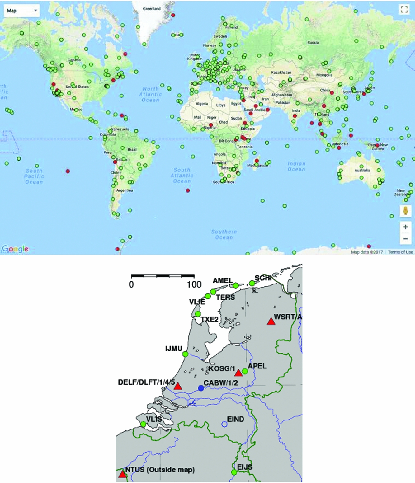
Fig. 13. Above, the GPS Network from the International GNSS Service (IGS), and below, a map with the IGS stations in the Netherlands (red triangles) and AGRS.NL stations (green dots). The AGRS.NL stations conform to IGS standards; the Dutch IGS stations are part of AGRS.NL. The AGRS.NL stations form the primary GNSS infrastructure in the Netherlands. AGRS.NL and IGS data are freely available (http://gnss1.tudelft.nl/dpga, www.igs.org/).
National coverage on a commercial basis was provided in 2005 by the roll-out of a network operated by the company 06-GPS, and is currently also offered by three other providers: LNR Net, NETPOS and Trimble VRS-Now. In these systems, data from the CORS stations are (i) streamed to a central processing facility, (ii) processed into correction data and then (iii) sent to the user using GSM or mobile Internet. The correction data are provided as, e.g., Virtual GNSS Reference Station (VRS) data: the user receiver first relays its rough position to the central position facility, and then receives tailor-made correction data from the central processing facility with all the appropriate corrections for its position. Data for these networks are also available for post-processing.
The non-commercial NETPOS data are only available to governmental agencies. The networks shown in Fig. 14 each consist of about 40–50 reference stations, some of which are shared among networks or with networks of neighbouring countries.
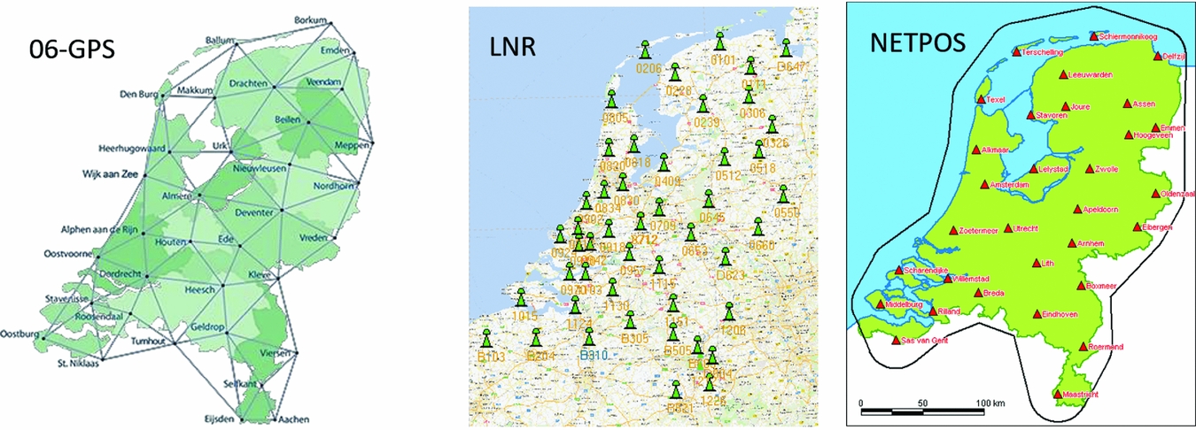
Fig. 14. RTK Networks in the Netherlands, with on the left the 06-GPS network, in the middle LNR-GlobalCom network, and on the right the NETPOS network.
The International GNSS Service (IGS) computes precise GNSS satellite orbits and clock corrections. It computes the precise coordinates of the IGS stations in the International Terrestrial Reference Frame (ITRF). Products from IGS that are important for deformation monitoring in the Wadden Sea area are
• continental, regional and national CORS networks. These networks always include data from several IGS stations to link these networks to the ITRF, and make use of other IGS products in the processing. Examples are the EUREF Permanent GNSS network (EPN) and the Dutch AGRS.NL network (Adam et al., Reference Adam, Augath, Boucher, Bruyninx, Dunkley, Gubler, Gurther, Hornik, van der Marel, Schluter, Seeger, Vermeer, Zielinski and Schwarz2000; De Bruijne et al., Reference De Bruijne, van Buren, Kösters and van der Marel2005).
• GNSS campaigns. These use IGS station data, precise orbits and station coordinates and velocities, to link the campaign to the ITRF. Examples are the EUREF campaigns for reference frame densification (Adam et al., Reference Adam, Augath, Boucher, Bruyninx, Dunkley, Gubler, Gurther, Hornik, van der Marel, Schluter, Seeger, Vermeer, Zielinski and Schwarz2000), and repeat campaigns for subsidence, tectonic and volcano monitoring (Bock & Melgar, Reference Bock and Melgar2016).
• Precise Point Positioning (PPP). This uses IGS satellite orbits and clocks to compute millimetre to centimetre accuracy positions for a single receiver (Zumberge et al., Reference Zumberge, Heflin, Jefferson, Watkins and Webb1997). This mode is supported by most scientific GNSS software analysis packages and often delivers results equally good as a full network adjustment. It is also offered as a service on the Internet: after the user uploads the receiver files, the file is processed on a server, and the computed coordinates are returned to the user.
AGRS.NL and IGS data are used by the Dutch Cadaster for the certification of Network RTK stations. This ensures that all Network RTK providers provide correction data in the same reference frame: the European Terrestrial Reference System 1989 (ETRS89/ETRF2000), which is the official reference frame for Europe (De Bruijne et al., Reference De Bruijne, van Buren, Kösters and van der Marel2005).
Continuously operating GNSS monitor stations and campaign stations can be used for subsidence and ground deformation monitoring. These stations are not very different from CORS or other GNSS campaign stations, except that the stations are now purposely not located in stable areas but in the study area for the subsidence or ground deformation. The data of the monitor stations can be processed like other CORS and campaign stations, using, e.g., data from the IGS or related networks as stable reference points, or directly using PPP to compute the deformation time series (see e.g. Van der Marel et al., Reference Van der Marel, van Leijen, Hanssen, Bekendam, Heitfeld, Rosner, Pietralla and Rosin2016). This type of processing is well suited for areas with few other GNSS reference stations. For the Wadden Sea area also, dense RTK networks can be used for the post-processing of the monitoring station data, with very good results (see also ‘Data availability in the Wadden Sea’ below).
Similar to the discussion in ‘Surface measurement vs the signal of interest’ above, the actual foundation of the benchmark for the GNSS antenna is relevant to the observable deformation (see the discussion on idealisation accuracy).
InSAR/PSI
Satellite radar interferometry (InSAR) is a technique based on repeated imaging radar acquisitions. Synthetic aperture radar (SAR) satellites are orbiting the Earth, and actively transmit radar signals to the Earth's surface. Parts of these signals are received back at the satellite. Fig. 15, left, shows an example of the recorded reflection strength for a SAR acquisition over an urban area, acquired by the TerraSAR-X satellite. Apart from the reflection strength, the fractional phase of the incoming electro-magnetic wave is also recorded. Hereby, a range-dependent measure is obtained. By taking the difference in phase between two acquisitions at different epochs, an interferogram is obtained, showing the combined effect of surface motion, topography and atmospheric signal delay (see Fig. 15, right). An overview of the most important SAR satellite missions for surface motion monitoring is given in Table 3.
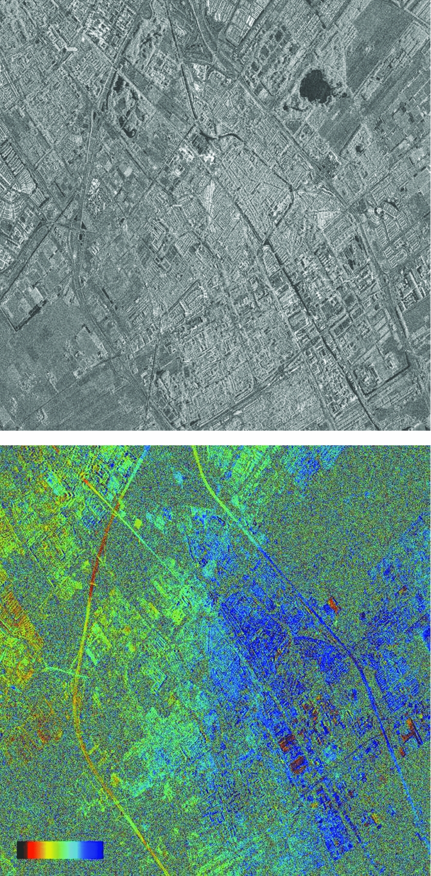
Fig. 15. SAR amplitude image of Delft (TSX satellite). The grey scale indicates the strength of the radar reflection. Black indicates a low reflection, e.g. due to specular reflection by the water in the lake. White indicates strong reflection, e.g. due to buildings. Right: Interferogram based on the phase of two SAR images. The colour cycle indicates the difference in path length between the surface and the satellite during the two acquisitions, due to deformation, topography and atmospheric signal delays.
Table 3. Most important SAR satellite missions for surface motion monitoring and their characteristics.
To enable the estimation and removal of the topographic and atmospheric phase contribution from the interferometric phases, interferometric time series methods are developed. Hereby, a large stack of SAR acquisitions acquired by the same satellite from the same orbital position are analysed simultaneously. Two approaches were developed: the Small BAseline Subset (SBAS) (Berardino et al., Reference Berardino, Fornaro, Lanari and Sansosti2002; Mora et al., Reference Mora, Mallorqui and Broquetas2003) and the Persistent Scatterer Interferometry (PSI) approach (Ferretti et al., Reference Ferretti, Prati and Rocca2000, Reference Ferretti, Prati and Rocca2001). The SBAS approach requires a spatially coherent signal, denoted as distributed scattering (DS).
Typically, an averaging of multiple image pixels is applied to reduce the noise. However, for large areas with vegetation, such as agricultural fields, this standard averaging approach is not sufficient and the SBAS methodology cannot be applied successfully (see also Fig. 15, right). Therefore, in the Netherlands, especially the PSI technique was applied. The PSI approach is based on the detection of points in the interferometric data stack with a consistent reflection over time. These points, so-called Persistent Scatterers (PS), are often located at man-made objects, such as buildings and different types of infrastructure.
More recently, hybrid methods have been developed to harmonise the strengths of both the SBAS and the PSI techniques (see e.g. Hooper, Reference Hooper2008; Ferretti et al., Reference Ferretti, Fumagalli, Novali, Prati, Rocca and Rucci2011; Samiei-Esfahany et al., Reference Samiei-Esfahany, Esteves Martins, van Leijen and Hanssen2016; Samiei-Esfahany, Reference Samiei-Esfahany2017). For instance, instead of multi-looking over fixed rectangular areas, averaging over homogeneous subsets of pixels can be performed.
Moreover, by estimating a coherence matrix per pixel (subset), a weighting of the different acquisitions can be applied. For instance, in case of grass fields, acquisitions in winter time get higher weights compared to summer images. Hereby, it has become possible to obtain first results regarding the subsidence of agricultural fields (see Fig. 16) (Morishita & Hanssen, Reference Morishita and Hanssen2015a,b; Samiei-Esfahany et al., Reference Samiei-Esfahany, Esteves Martins, van Leijen and Hanssen2016). Since these new hybrid approaches are often implemented in a PSI framework, to combine the estimation and detection of Persistent Scatterers as well as Distributed Scatterers, henceforth we will refer to these optimised approaches as Persistent Scatterer Interferometry (PSI). See Crosetto et al. (Reference Crosetto, Monserrat, Cuevas-González, Devanthéry and Crippa2016) for a review of PSI.

Fig. 16. Subsidence in the rural area of Delfland, south of Delft, the Netherlands, based on InSAR. The area within the green polygon mainly consists of pasture fields. Left: Linear subsidence rate (mma −1). Right: Amplitude of the periodic annual signal (mm) (Morishita & Hanssen, Reference Morishita and Hanssen2015b).
The PSI technique can be applied for various applications. In the Netherlands, PSI is used to measure surface motion due to gas extraction (Ketelaar, Reference Ketelaar2009), abandoned mining (Caro Cuenca et al., Reference Caro Cuenca, Hooper and Hanssen2013), sinkhole detection (Chang & Hanssen, Reference Chang and Hanssen2014), groundwater extraction (Van Leijen & Hanssen, Reference Van Leijen and Hanssen2008), railway monitoring (Chang et al., Reference Chang, Dollevoet and Hanssen2015, Reference Chang, Dollevoet and Hanssen2017) and water defence structure monitoring (Hanssen & van Leijen, Reference Hanssen and van Leijen2008; Van Leijen et al., Reference Van Leijen, Humme, Hanssen, Barends, Dillingh, Hanssen and van Onselen2008).
A PSI analysis results in estimated time series for each detected Persistent Scatterer. To enable the estimation of the phase ambiguities, that is, to estimate the unknown number of full phase cycles in the deformation time series, a deformation model is used. As a null hypothesis, often a steady-state deformation model is used. However, in case of nonlinear motion, this model may result in a biased estimation of deformation rates. As a consequence, PS may not be detected, or biased time series are obtained. To increase the reliability in the estimated deformation time series and the number of detected PS, alternative deformation models can be tested (Van Leijen & Hanssen, Reference Van Leijen, Hanssen, Lacoste and Ouwehand2007a,b). Alternative models can for instance contain a breakpoint, a step or a higher-order polynomial. Also temperature effects, for instance due to thermal expansion of buildings, can be modelled (Monserrat et al., Reference Monserrat, Crosetto, Cuevas and Crippa2011).
Alternatively, a library of alternative deformation models can be tested as a post-processing step, based on the estimated time series using an initial linear model (Chang & Hanssen, Reference Hanssen2015). This approach is possible because the phase ambiguities are typically estimated for arcs between nearby PS. Hence, on short distance, an initial linear model is often valid.
Although the deformation time series is the prime outcome of a PS analysis, for visualisation properties often the linear deformation rates are shown. An example is shown in Fig. 17 for the region of Delfland, based on data acquired between 1992 and 2000 by the ERS satellites.
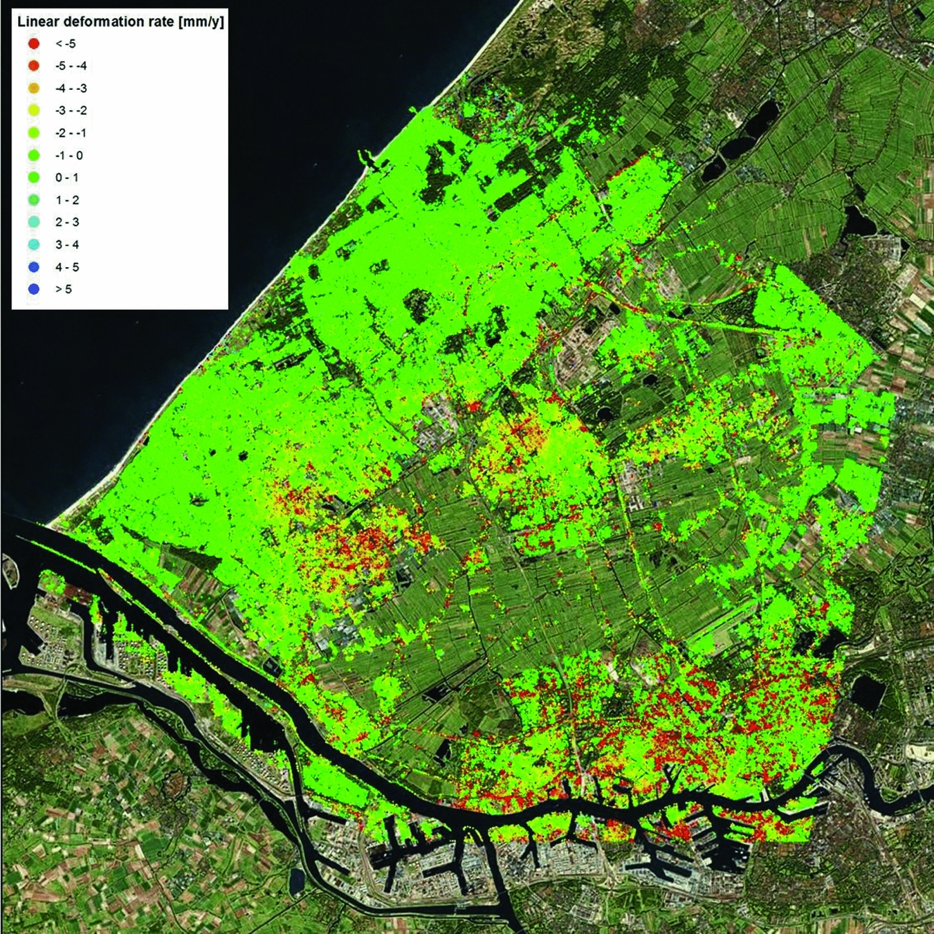
Fig. 17. Linear surface motion rates (mma−1) in vertical direction in Delfland obtained by Persistent Scatterer Interferometry, based on data acquired by the ERS satellites (1992–2000).
Together with the relative surface motion time series, i.e. height difference changes over time, the height differences between PS are estimated. These estimates are less precise than the differential height change estimates. The standard deviation of the height difference estimates is better than 1m for X-band data (~3cm wavelength; see Table 3), and 1–2m for C-band data (~6cm wavelength) (Crosetto et al., Reference Crosetto, Monserrat, Bremmer, Hanssen, Capes and Marsh2009).
The estimated height differences are important for the further analysis of the PSI results for two reasons. First, since the radar measurement is taken under an angle with respect to nadir, known as the incidence angle, the height has a direct influence on the georeferencing (planar coordinates) of the PS. Hence, the accuracy of the height difference estimates directly translates to the positioning accuracy, dependent on the incidence angle. For example, for ERS/Envisat datasets with an incidence angle of about 26°, this results in a standard deviation of the X,Y-position of 2–5m (Crosetto et al., Reference Crosetto, Monserrat, Bremmer, Hanssen, Capes and Marsh2009). The positioning of the PS is important to determine the origin of the radar reflection, and thereby for the interpretation of the PSI results.
Secondly, the estimated height differences between the PS can be used to separate reflections from surface level from those originating from objects. As discussed in the section ‘Surface measurements vs the signal of interest’ above, the sensitivity of a measurement for a certain deformation signal depends on the foundation of that benchmark, or in this case the reflection, involved. This is illustrated in Fig. 18, assuming that all buildings in a certain area have a foundation on a deeper support stratum. The dihedral reflections, via the wall of a building and the surface, measure the surface motion, whereas the specular reflections from buildings are only sensitive to motion of the foundation layer and below. Using the estimated PS height differences, these two groups of reflections can be separated, and the effects of shallow and deep compaction can be isolated. An illustration of this approach for the city of Diemen, the Netherlands, is given in Fig. 19.
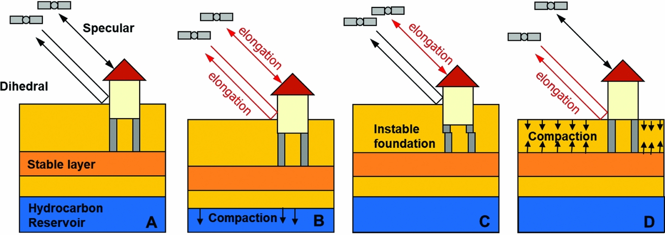
Fig. 18. Sensitivity of PSI measurements for different deformation regimes. (A) Dihedral wall-surface reflections are sensitive to motion of the surface layer and deeper layers, whereas, in case of deep foundations, specular reflections from objects are only sensitive to motion of the foundation layer due to deep processes. (B) The effect of deep compaction, measured by both the dihedral and specular reflections. (C) The effect of an instable foundation, only measured by the specular reflections. (D) The effect of shallow compaction, only measured by the dihedral reflections.
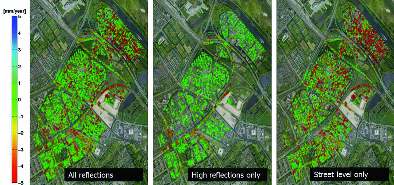
Fig. 19. Example of the separation of high and low reflection points, to distinguish shallow and deep compaction processes for the city of Diemen, the Netherlands, based on TerraSAR-X satellite data (2009–2014). Left: Linear deformation rates of all PS. Middle: Linear deformation rates of only high reflection points, showing the motion of the foundation layer (deep processes). Right: Linear deformation rates of only the low reflection points, showing the effect of shallow compaction. Courtesy: SkyGeo Netherlands.
One of the strengths of PSI is that thousands of measurement points can be obtained per km2 (see Table 3), without any installation requirements on the surface. Due to the relative nature of the technique, both in space and in time, and the arbitrary references chosen, the measurements are not connected to a predefined geodetic datum. To connect the PSI measurements to a datum, a datum connection approach using for instance GNSS and/or levelling data can be applied (see next section). Such an approach has the advantage that systematic spatial trends in the estimated solution, for instance due to orbit errors (Bähr & Hanssen, Reference Bähr and Hanssen2012) or atmospheric signal delays (Hanssen, Reference Hanssen2001), can be removed. This is particularly useful for the analysis of large areas. On a local scale, the effects of these error sources are negligible.
Since PSI points and GNSS/levelling benchmarks are not collocated, a spatial interpolation is required to perform such a datum connection. An alternative approach is the use of corner reflectors or active radar transponders, with a fixed connection to a GNSS/levelling benchmark. The development of active transponders is relatively new. Their performance was tested by Mahapatra et al. (Reference Mahapatra, Samiei Esfahany, van der Marel and Hanssen2013, Reference Mahapatra, van der Marel, van Leijen, Samiei Esfahany, Klees and Hanssen2017). These transponders transmit the radar signal, and thereby form an artificial ‘controlled’ PS. By co-locating a transponder with a GNSS receiver, both measurement techniques can be connected without any form of interpolation or assumptions. Hereby, the PSI measurements can be transformed into the same geodetic datum as the GNSS measurements. An example of such a set-up in IJmuiden, the Netherlands, is given in Fig. 20. Apart from application of transponders for datum connection, the transponders can also be used to create PS at locations where no suitable natural radar reflections are obtained (Mahapatra et al., Reference Mahapatra, Samiei-Esfahany and Hanssen2015).
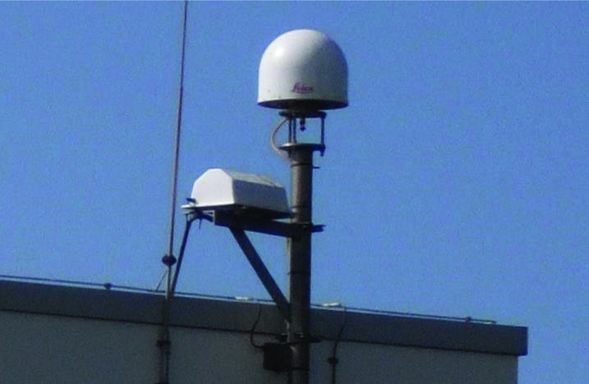
Fig. 20. GNSS station at IJmuiden, the Netherlands, with a co-located active radar transponder. Hereby, GNSS measurements and PSI measurements can be connected in the same geodetic datum. The GNSS receiver is placed within the round dome, whereas the radar transponder is contained within the white box.
In early 2018, a system of 28 Integrated Geodetic Reference Stations (IGRS) was installed, which combines a GNSS antenna, InSAR double corner reflectors, an airborne laser scanning benchmark and a levelling benchmark (Hanssen, Reference Hanssen2017) (see Fig. 21). These stations serve both to provide an accurate and collocated height reference benchmark for calibration, as well as sufficient redundancy for quality control.
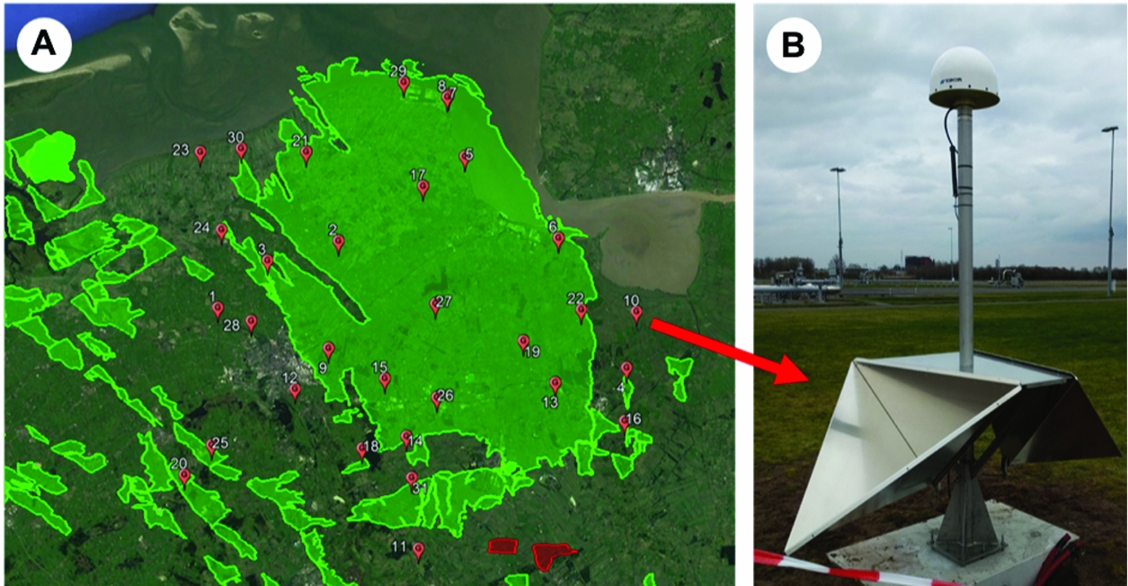
Fig. 21. Deployment of Integrated Geodetic Reference Stations (Hanssen, Reference Hanssen2017) over the Groningen region. These stations serve as a reference for height and deformation calibration and to cross-validate the results of various techniques.
Data integration
The various measurement techniques have their own characteristics, as discussed in ‘Surface measurements vs the signal of interest’ above. The resulting datasets are therefore different and complementary. These differences reflect themselves in for instance the spatial density and extent, temporal sampling and extent, precision, sensitivity direction and reference system of the data. Because of their complementarity, the integration of the various datasets is desirable. For future applications, a monitoring set-up taking these varying characteristics of the different techniques can be designed. For example, by assessing the expected PSI/InSAR point density in urban and rural areas, the number and distribution of GNSS and/or levelling benchmarks (and measurement frequency) can be optimised accordingly. For analysis of the past situation, in principle all the available data should be considered to assess their impact.
Caro Cuenca et al. (Reference Caro Cuenca, Hanssen, Hooper and Arikan2011) performed an integration of levelling, GNSS, gravimetry and InSAR data for the whole of the Netherlands. The spatial distribution of the measurement points is shown in Fig. 22. Here, the integration was based on the linear deformation rates derived from the time series of the various techniques. By using linear deformation rates, the problem of the different measurement epochs is circumvented. In the spatial domain, the integration was based on an interpolation of the linear deformation rates per technique to a common grid using kriging. The kriging is based on a covariance function estimated from the data. Hereby, the spatial smoothness and the noise level of the data are considered, and a precision estimate per grid cell is obtained. Finally, a least-squares inversion is applied to estimate offsets between the various techniques and the final deformation map. To enable the separation of deep and shallow compaction effects, for each technique involved the measurement points are separated into two groups: points with and without a deep foundation. The resulting surface motion maps, together with their standard deviations, are shown in Fig. 23 for the shallow compaction, in Fig. 24 for the deep compaction, and in Fig. 25 for the total surface motion. A similar integration approach is applied by Fuhrmann et al. (Reference Fuhrmann, Caro Cuenca, Knöpfler, van Leijen, Mayer, Westerhaus, Hanssen and Heck2013, Reference Fuhrmann, Caro Cuenca, Knöpfler, van Leijen, Mayer, Westerhaus, Hanssen and Heck2015) for the Upper Rhine Graben in Germany.
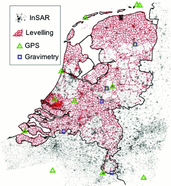
Fig. 22. Spatial distribution of measurement points of various techniques used to create a nationwide ground motion map of the Netherlands (Caro Cuenca et al., Reference Caro Cuenca, Hanssen, Hooper and Arikan2011).
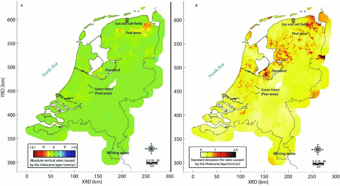
Fig. 23. Linear deformation rates (A) and their standard deviation (B) over the whole of the Netherlands caused by shallow compaction (Caro Cuenca et al., Reference Caro Cuenca, Hanssen, Hooper and Arikan2011).
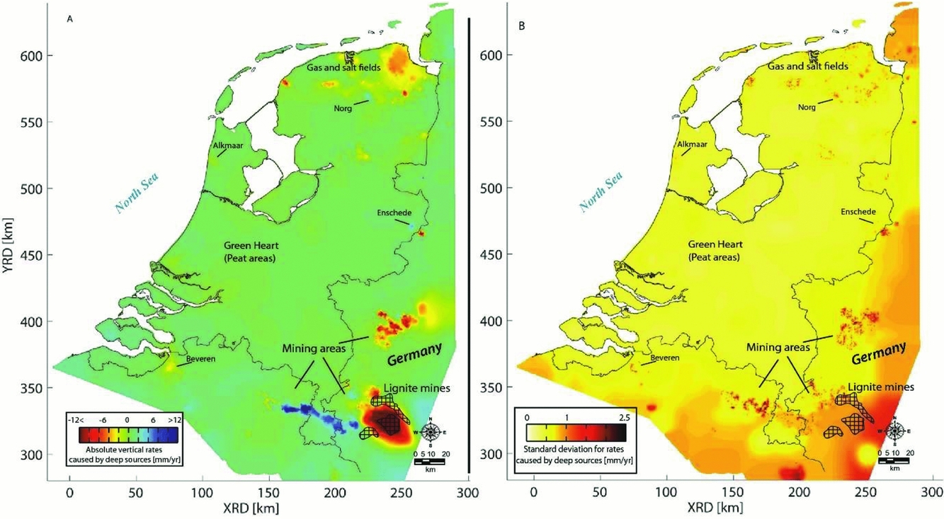
Fig. 24. Linear deformation rates (A) and their standard deviation (B) over the whole of the Netherlands caused by deep compaction (Caro Cuenca et al., Reference Caro Cuenca, Hanssen, Hooper and Arikan2011).
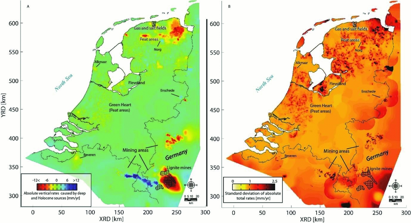
Fig. 25. Total linear deformation rates (A) and their standard deviation (B) over the whole of the Netherlands (Caro Cuenca et al., Reference Caro Cuenca, Hanssen, Hooper and Arikan2011).
Van der Marel et al. (Reference Van der Marel, van Leijen, Hanssen, Bekendam, Heitfeld, Rosner, Pietralla and Rosin2016) applied a data integration for the Limburg mining area based on spatial kriging of the original deformation time series. Alternatively, the integration can be performed in the model space (see Fokker & Van Thienen-Visser, Reference Fokker and Van Thienen-Visser2016; Fokker et al., Reference Fokker, Wassing, van Leijen, Hanssen and Nieuwland2016). This approach is further discussed in the next section.
Data availability in the Wadden Sea region
Optical and hydrostatic levelling
The historic optical and hydrostatic levelling measurements in the Netherlands are archived in the ‘Hoogte Informatie Systeem’ (HIS) of Rijkswaterstaat. This database contains the measurements of the second (around 1930) until fifth (around 1995) precision levelling (Nauwkeurigheidswaterpassing), the measurements for the maintenance of the secondary NAP benchmark network, and levelling measurement campaigns by third parties. The availability of the original measurements makes it possible to reassess the data from an elementary level, for instance in a combined temporal–spatial analysis. The measurements of the first precision levelling are largely lost, but the adjusted heights are still available (Brand, Reference Brand2002). Third-party levelling campaigns are mainly associated with mining activities. Mining companies are obliged by Dutch law to monitor the effect of their extraction on the surface subsidence. Examples are the mining regions in Limburg, oil and gas fields, and salt extraction sites.
The locations of the NAP benchmarks and their latest annotated height are made available via Publieke Dienstverlening Op de Kaart (PDOK) (www.pdok.nl). Fig. 26 shows the NAP benchmarks in the wider Wadden Sea area.
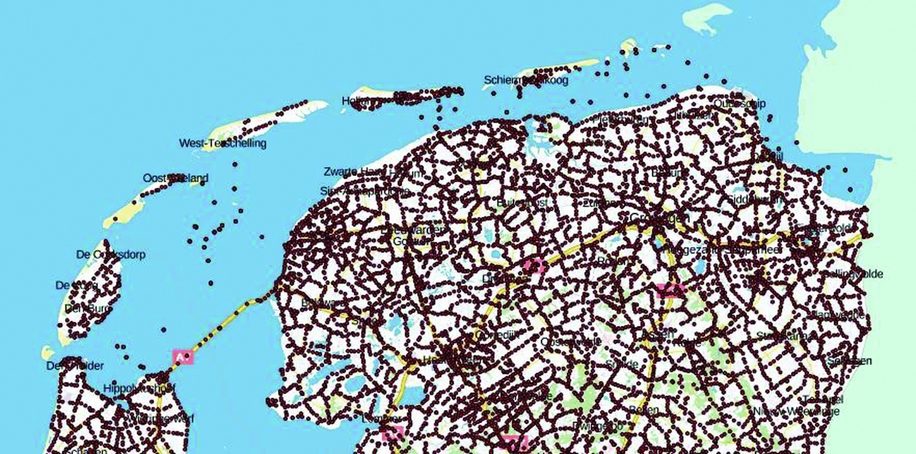
Fig. 26. Location of the NAP benchmarks in the Wadden Sea area. For each benchmark, the latest surveyed NAP height and the location of the benchmark is given. From http://pdokviewer.pdok.nl/, visited 12 September 2017.
As an example, the levelling data availability in the region around Ameland since 1986 is given in Table 4. The measurements are taken during campaigns, typically spanning weeks to months. Both optical and hydrostatic levelling data are available in this case. The measurements are acquired both by Rijkswaterstaat and by the Nederlandse Aardolie Maatschappij (NAM), because of mining activities in the region.
Table 4. Example of the available levelling campaigns for the region around Ameland since 1986. The campaigns contain both optical and hydrostatic levelling measurements. The measurement campaigns are performed both by Rijkswaterstaat and the Nederlandse Aardolie Maatschappij (NAM), because of mining activities in the region. (Dates are day-month-year.)
GNSS
Fig. 27 shows the available GNSS data in the Wadden Sea area: Continuously Operating GNSS Reference Stations from AGRS.NL and Network RTK providers, continuously operating GNSS monitor stations, and campaign monitor stations in and around the gas fields.
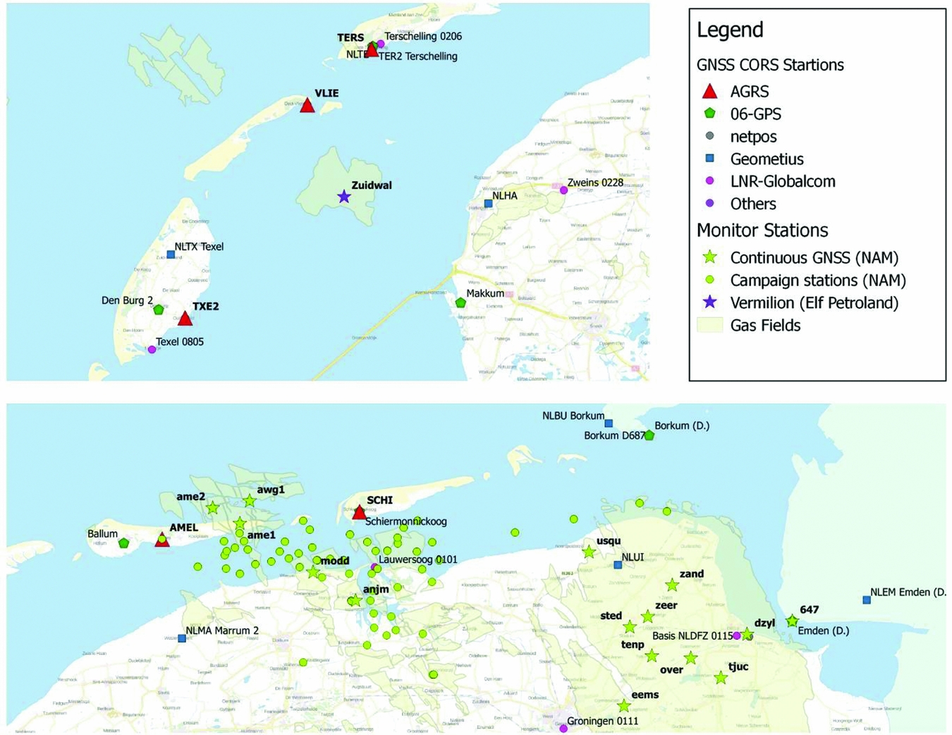
Fig. 27. GNSS data availability in the Wadden Sea area, showing the available GNSS Continuously Operating Reference Stations (CORS) from various service providers, and continuously operating monitor stations and campaign stations in and around the gas fields.
The GPS on the Zuidwal platform (PE-ZW-PA) is one of the oldest GPS monitor stations in the area. Exploitation of the Zuidwal platform was started in 1988 by Elf Petroland, now Vermilion Energy. The subsidence was initially monitored by optical and hydrostatic levelling, but was replaced by GPS. The other GPS monitor stations are managed by NAM and the data are processed by 06-GPS.
In 2006, NAM installed three continuously operating GPS monitor stations at Ameland-East (AME1), Moddergat (MODD) and Anjum (ANJM), followed in 2014 by the installation of continuously operating GPS monitor stations on the platforms AWG-1 and AME-2.
Before the installation of continuously operating monitor stations in 2014, AWG-1 and AME-2 were observed by regular GPS campaigns in 1993, 1997, 1998, 2000 and 2004 using GPS short baseline measurements with three to four receivers with a measurement period of several hours. Typical baselines were 3–4km long, with a longest baseline of 10.7km. After 2006, AWG-1 and AME-2 were included in regular GPS campaigns, until they became CORS stations in 2014. In 2006 NAM also started new GPS campaigns. These campaigns are repeated more or less every year since 2006 and include over 70 points in the Wadden Sea, on the platforms and onshore. For the campaigns the same equipment is used as the GPS monitor stations, collecting typically 5 days of observations per point. Four to five campaign points are observed simultaneously. After 5 days the equipment is relocated to another point. Campaigns can last up to one month, but some have been split over several shorter periods. Not every campaign point is observed each year. In total about 150 benchmarks, at just under 70 locations, have been observed during one or more GPS campaigns. Some of the benchmarks, mainly in the Wadden Sea area, are located in 40 clusters of typically three benchmarks each. Only one of these benchmarks is observed with GPS. The other benchmarks in the cluster are connected by levelling to the GPS benchmark. A typical benchmark in the Wadden Sea, and set-up of the GPS receiver and antenna, is shown in Fig. 28. The set-up of the GPS antenna is such that only the height component is repeatable over time. The horizontal components cannot be used for monitoring (Van Leijen et al., Reference Van Leijen, Samiei Esfahany, van der Marel and Hanssen2017).
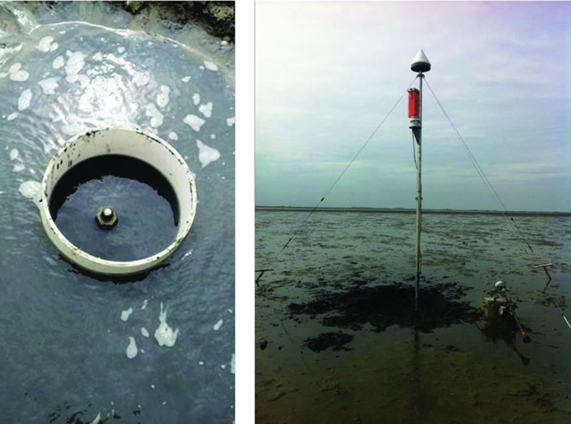
Fig. 28. Typical GPS benchmark (left) and GPS measurement set-up (right) in the Wadden Sea area (pictures courtesy NAM).
Typical of the 06-GPS processing is that the GPS monitor station and campaign data are processed together. Therefore, the results for the GPS monitor stations and campaign data in the area of interest are very homogeneous. The 06-GPS processing also includes several continuously operating GPS stations from outside the area of interest, the so-called GPS reference stations, of which the coordinates are constrained to reference values. The GPS reference stations provide a stable reference frame for the stations in the area of interest.
There have been occasional updates of the reference station coordinates and changes in the set of reference stations (06-GPS, 2015). For the processing the GNSMART software is used, giving mm accurate results (Geo++, 2006a,b; 06-GPS, 2016). GNSMART stands for GNSS State Monitoring and Representation Technique. A complete state-space model (SSM) with millimetre accuracy is implemented for the rigorous and simultaneous adjustment of GNSS observables, which is essential to resolve phase ambiguities, as well to mitigate major GNSS error sources. For the receiver coordinates various models are used: fixed coordinates for GPS reference stations, dynamic (filtered) for GPS monitor stations and epoch-wise for campaign stations. The adjustment model is a Kalman filter (Geo++, 2006a,b), running in post-processing mode, using IGS Ultra rapid Precise orbits (Dow et al., Reference Dow, Neilan and Rizos2009). The data are processed in periods of one and a half months, with an overlap of half a month. The first half-month is used for the Kalman filter to obtain a steady state and is not used for the final solution. Therefore, each run results in a one-month final solution. The coordinates are computed with an interval of 1 hour (06-GPS, 2016).
The results from the 06-GPS processing are further processed by software developed by TU Delft for NAM (Van Leijen et al., Reference Van Leijen, Samiei Esfahany, van der Marel and Hanssen2017). The objective of the software is:
• Decompose the continuous monitoring station time series into components including a secular trend, temperature influence, atmospheric loading, harmonic components, jumps and noise components; remove the components not related to ground deformation to obtain a clean series.
• Subsample the cleaned time series into one data point per year, coinciding with the mean epoch of the campaign measurements.
• Provide temperature corrections for the AWG-1 and AME-2 campaign measurements.
• Combine GPS and levelling data of the campaign clusters, and remove outliers.
• Compute the covariance matrix for the continuously operating and campaign monitoring stations using the model developed by Williams (Reference Williams2015).
The results are saved in the CUPiDO NetCDF format (Van Leijen et al., Reference Van Leijen, Samiei Esfahany, van der Marel and Hanssen2017).
InSAR
The crucial factor regarding availability of InSAR data is whether or not the SAR images are actually acquired. Based on the archived SAR data, a new PSI analysis can always be performed. Data availability is not guaranteed, because some of the SAR missions are operated commercially, and acquisitions are only taken based on customer request. For other missions, operated by the European Space Agency (ESA), such as ERS, Envisat and Sentinel-1, the SAR imagery is acquired on a more systematic basis. The data availability of the Wadden Sea region is summarised in Table 5. The table shows that the first data are available from 1992. With the data acquired by the ERS, Envisat, RadarSAT-2 and Sentinel-1 missions, a more or less continuous coverage of data is obtained for the last 25 years (1992–2017). The availability of the commercial RadarSAT-2 data is established by the Dutch government, organised by the Netherlands Space Office (see www.spaceoffice.nl/nl/satellietdataportaal/).
Table 5. Availability of SAR data for the Wadden Sea area.
Fig. 29 shows an example of PSI-based surface deformation at Groningen. Wadden Sea coastlines are indicated with dashed lines (Hanssen, Reference Hanssen2015). The figure also shows gradients in the deformation field, as well as a time-series example for one of the gas production stations.
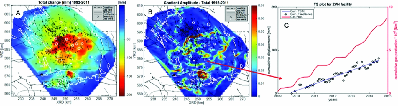
Fig. 29. PSI-based surface displacement estimates 1992–2011 (ERS-1/2 data). (A) InSAR cumulative vertical displacement, with overlaid Wadden Sea coastlines (dashed), gas reservoir boundaries (white), faults (black), earthquakes (black circles) and gas wells (black). (B) gradient amplitudes, outlining different compartments (pockets) of deformation (spatial variability). (c) Temporal variability of gas production (red) and InSAR time series for the Zuiderveen facility, showing strong correlation between production and surface deformation (Hanssen, Reference Hanssen2015).
Combining models and measurements
Inverse modelling and data assimilation
As outlined in the previous sections, the surface movement constitutes a measurable signature of the processes in the reservoir. Such measurements can thus provide information about the subsurface (Maury et al., Reference Maury, Grasso and Wittllinger1992). However, large uncertainties are usually associated with subsurface parameters. Without being exhaustive, typical uncertainties include the value of the compaction coefficient of the reservoir rock and its dependence on porosity and pressure (Van Thienen-Visser & Fokker, Reference Van Thienen-Visser and Fokker2017); time dependence of compaction; the geomechanical response of the reservoir surroundings up to the surface; interfering causes such as deep and shallow expressions of compaction; and the amount of aquifer activity.
Uncertainties in subsurface parameters result in considerable uncertainties in the associated surface movement forecasts.
Inverse modelling or data assimilation is required to successfully constrain subsurface knowledge and parameters with the use of surface movement data (Tarantola, Reference Tarantola2005), but this is not straightforward. Such an endeavour is especially difficult for the combination of a spatially distributed source of compaction such as a gas field, strongly nonlinear forward models, interfering causes of subsidence and highly correlated data (see Fig. 30). The solution is often not unique or not stable – ill-conditioned in mathematical terms. Then, additional information is required to obtain a stable solution. This is called regularisation of the inverse problem. We will briefly sketch how inverse modelling of subsidence has developed over the last few decades; in the next section we will highlight this with some published field studies.
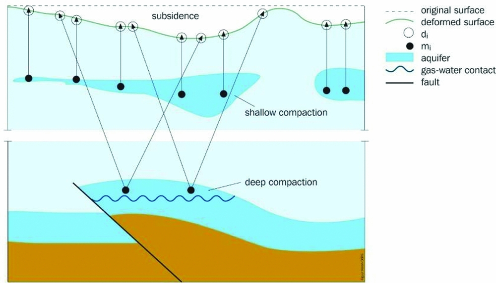
Fig. 30. Demonstration of compaction sources leading to a cumulative and smoothed subsidence expression.
Some early attempts to use inverse modelling to relate surface movement data to reservoir properties employed linear forward models and no prior knowledge of the reservoir pressure distribution (Mossop & Segall, Reference Mossop and Segall1999; Du & Olson, Reference Du and Olson2001; Dusseault & Rothenburg, Reference Dusseault and Rothenburg2002; Fokker, Reference Fokker2002; Du et al., Reference Du, Brissenden, McGillivray, Bourne, Hofstra, Davis and Wright2008). In these studies, the investigators typically reverted to regularisation methods such as smoothness constraints to handle the ill-conditioning that results from compaction having a large radius of influence on surface movement.
A better way to regularise the inversion is to use direct prior knowledge, such as information on the pressure distribution. Marchina (Reference Marchina1996) described this procedure and attempted to apply it to the Groningen gas field. Matsuura et al. (Reference Matsuura, Noda and Fukahata2007) applied a similar approach to slip behaviour during an earthquake and included indirect knowledge such as the smoothness of the slip distribution. Muntendam-Bos et al. (Reference Muntendam-Bos, Kroon and Fokker2008) and Fokker et al. (Reference Fokker, Visser, Peters, Kunakbayeva and Muntendam-Bos2012) followed the same approach, using all available information from geological and reservoir modelling.
If nonlinearities are incorporated in the forward model, linear inversion cannot be used.
One alternative, especially when coupled numerical modelling is involved, is to revert to classical history matching (Vasco et al., Reference Vasco, Karasaki and Doughty2000, Reference Vasco, Ferretti and Novali2008, Reference Vasco, Rutqvist, Ferretti, Rucci, Bellotti, Dobson and Hartline2013), which is an example of deterministic inverse modelling. If fewer parameters need to be estimated, an iterative least-squares approach may be appropriate (Vasco et al., Reference Vasco, Rucci, Ferretti, Novali, Bissell, Ringrose and Wright2010; Teatini et al., Reference Teatini, Castelletto, Ferronato, Gambolati, Janna, Cairo and Bottazzi2011; Rucci et al., Reference Rucci, Vasco and Novali2013). When data from other sources are input, and if systems have many parameters, ensemble-based methods may be employed. An ensemble-based modelling approach for the Wadden Sea (Van Thienen-Visser et al., Reference Van Thienen-Visser, Breunese and Muntendam-Bos2015) will be discussed in the context of the discussion of the Wadden Sea gas fields in the section ’Salt solution mining in Havenmond’ below. A study employing an Ensemble Kalman filter (EnKF) was reported by Chang et al. (Reference Chang, Chen and Zhang2010). The application was on a synthetic model with production data and surface movement data, but they did not capture the main features of the spatial pattern of the Young's modulus, possibly because the subsidence levels were not sensitive to the distribution of the moduli. Wilschut et al. (Reference Wilschut, Peters, Visser, Fokker and van Hooff2011) applied EnKF on a field case and showed its usefulness on a synthetic dataset, but they failed to improve overall understanding of the actual data: the different types of data pointed to different geological interpretations. This was presumably because they had not taken account of the uncertainty of some of the parameters. The combined uncertainty of the vertical modulus profile and the compaction coefficient is hard to capture: the surface movement pattern is a complex function of the 3D geological setting, the spatial distribution of hydro-geomechanical properties, and changes in the effective stress induced by fluid extraction.
EnKF has been applied in other subsurface applications (Evensen, Reference Evensen2009) but it is not the only option for parameter estimation or data assimilation. An alternative is an Ensemble Smoother, which estimates parameters in a single step (Baù et al., Reference Baù, Ferronato, Gambolati, Teatini and Alzraiee2015). When applied with nonlinear forward models or non-Gaussian statistics, however, results are inferior to those obtained using EnKF (Tavakoli et al., Reference Tavakoli, Yoon, Delshad, ElSheikh, Wheeler and Arnold2013). Two publications by Emerick & Reynolds (Reference Emerick and Reynolds2013a,b) and by Tavakoli et al. (Reference Tavakoli, Yoon, Delshad, ElSheikh, Wheeler and Arnold2013) compare different ensemble techniques and conclude that an Ensemble Smoother with Multiple Data Assimilation is a good alternative: computational cost is like that of EnKF but the result of ES-MDA is better in the sense of agreement with the ‘true’ model in their synthetic cases. The ES-MDA schedule was followed by Fokker et al. (Reference Fokker, Wassing, van Leijen, Hanssen and Nieuwland2016).
Yet another approach is to use a so-called particle filter (Van Leeuwen, Reference Van Leeuwen2009) which was developed for use in subsidence monitoring and control by Nepveu et al. (Reference Nepveu, Kroon and Fokker2010). The method also employs a stochastic approach: many subsurface model realisations are created to calculate an equal number of subsidence predictions. The ensemble of all realisations should map the prior uncertainties of the model parameters to a range of subsidence predictions. These predictions are then compared with the measured values. For every single realisation, the discrepancy between measurements and data is used to estimate a probability that that realisation is representative for the reality. A posterior model estimate is finally constructed by means of a weighted average of all prior forecast realisations – the weights being the probabilities determined in the previous step. The attraction of this approach is that model realisations do not have to be updated: the prior models are used to estimate an improved model forecast. However, the problem with the method is that with many measurement points a tendency to divergence or ensemble collapse emerges: one single model will collect virtually all the weight, and the prediction coincides with the prediction of that model only. This behaviour also renders the calculation of a posterior uncertainty range impossible. An unrealistic number of model realisations would be required to obtain a reasonable number of non-zero posterior weights (Van Leeuwen, Reference Van Leeuwen2009).
Persistent Scatterer InSAR (PS-InSAR) measurements result from the projection of the 3D deformation vector along the line of sight to the satellite (‘InSAR/PSI’ section above). Using ascending and descending satellite orbits, the deformation vector can be decomposed further, albeit still insufficiently for full decomposition in the north, east and vertically upwards directions. GPS provides movement in all three directions. Klemm et al. (Reference Klemm, Quseimi, Novali, Ferretti and Tamburini2010) have demonstrated the usefulness of PS-InSAR data from both ascending and descending orbits. Janna et al. (Reference Janna, Castelletto, Ferronato, Gambolati and Teatini2012) unravelled horizontal (east–west) and vertical movements from a series of PS-InSAR measurements and used them to calibrate a transversally isotropic geomechanical model of the subsurface around an underground gas storage field in northern Italy. The decomposition into vertical and east–west movements, however, introduces the need for an interpolation (Klemm et al., Reference Klemm, Quseimi, Novali, Ferretti and Tamburini2010; Janna et al., Reference Janna, Castelletto, Ferronato, Gambolati and Teatini2012; Rucci et al., Reference Rucci, Vasco and Novali2013), because the persistent scatterers identified for ascending and descending satellite orbits are not identical. Thus, such decomposition is allowed only when the deformation signal is sufficiently smooth and sufficiently well-sampled. Interpolation can be avoided by using the line-of-sight data directly in the parameter estimation procedure, as is common practice in the assessment of volcanic activity and earthquakes (Jónsson et al., Reference Jónsson, Zebker, Segall and Amelung2002; Anderssohn et al., Reference Anderssohn, Motagh, Walter, Rosenau, Kaufmann and Oncken2009). An assimilation schedule without decomposition was employed by Fokker et al. (Reference Fokker, Wassing, van Leijen, Hanssen and Nieuwland2016).
Example studies outside the Wadden Sea
Here, we summarise some findings obtained in hydrocarbon fields which are relevant to the Wadden Sea fields. It is by no means a comprehensive review, but rather some cases selected based on the findings connected to them. In the ‘Pitfalls’ section we will formulate learning points for the Wadden Sea, based on these cases. The Groningen field, which clearly contains many relevant lessons as well and contributes to the subsidence in the Wadden Sea area, will be discussed in the context of all the Wadden Sea fields in the section ‘Salt solution mining in Havenmond’ below.
Lacq
The Lacq gas field in southwestern France has been in production since 1957. The production caused both subsidence and seismicity, which triggered research in production-induced phenomena (Maury et al., Reference Maury, Grasso and Wittllinger1992; Bardainne et al., Reference Bardainne, Dubos-Sallée, Sénéchal, Gaillot and Perroud2008). Segall formulated a poroelastic description, and made an effort to relate the pressure reservoir drop to the subsidence measurements (Segall, Reference Segall1989, Reference Segall1992; Segall et al., Reference Segall, Grasso and Mossop1994). The profile that he observed was steeper than he could predict on the basis of a homogeneous elastic subsurface (Fig. 31). This he interpreted to be connected to the dome geometry of the gas-bearing layers, giving larger and steeper contributions to the subsidence of the central portions of the field. It is, however, difficult to judge the quality of the fit without a quality description of the data.
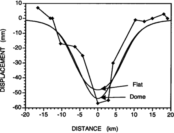
Fig. 31. Predicted vertical displacements at Lacq compared to levelling results for the time interval 1887–1989. Two predicted models are shown: one modelling the reservoir as a flat layer, and the second including the effect of the anticlinal dome structure (from Segall et al., Reference Segall, Grasso and Mossop1994).
Gulf Coast region
A large area in which many hydrocarbon fields are produced below low-lying wetlands is the US Gulf Coast region in coastal Louisiana and Texas (Morton et al., Reference Morton, Bernier and Barras2006; Yuill et al., Reference Yuill, Lavoie and Reed2009). Many processes contribute to the surface movement, similar to what is discussed in the present text. The complexity of the processes and the interference between different causes has made it difficult to come up with reliable predictive numerical modelling. Morton et al. (Reference Morton, Bernier and Barras2006) proposed to constrain to measurements and extrapolation. This seems to us a suboptimal approach since different physical mechanisms can lead to different future behaviours.
In Salah
The In Salah CO2 Storage Project in Algeria was in operation between 2004 and 2011 and was the first onshore, industrial-scale demonstration site for CO2 sequestration. Four million tons of carbon dioxide were injected into a 20-m thick, water-filled reservoir at a depth of about 2000m. The three injection wells were drilled horizontally with a length between 1 and 1.5km. A caprock with a thickness of about 900m prevented the CO2 from escaping to shallower depths (Ringrose et al., Reference Ringrose, Roberts, Gibson-Poole, Bond, Wightman, Taylor and Østmo2011; Rinaldi et al., Reference Rinaldi, Rutqvist, Finsterle and Liu2017).
The In Salah demonstration site is also well-known for the comprehensive characterisation and monitoring effort, including wellhead sampling, down-hole logging, core analysis, surface gas and groundwater aquifer monitoring, tracers, 4D seismic, and satellite InSAR data (Mathieson et al., Reference Mathieson, Midgley, Dodds, Wright, Ringrose and Saoul2010, Reference Mathieson, Midgely, Wright, Saoula and Ringrose2011). InSAR data provided essential information for the development of a reliable model through the inverse analysis of coupled fluid flow and geomechanics.
A key observation in the InSAR-derived surface movement at the In Salah site was a two-lobe surface heave structure in the northwestern direction above injection well KB-502. The observations, projected onto vertical and horizontal east–west movements, are reproduced in Fig. 32. It was recognised that this was the surface signature of a subsurface tensile fracture (Vasco et al., Reference Vasco, Rucci, Ferretti, Novali, Bissell, Ringrose and Wright2010; Rucci et al., Reference Rucci, Vasco and Novali2013). The authors performed an inverse analysis to estimate the characteristics of the subsurface behaviour. They constructed an earth model by using the seismic velocities of the subsurface strata, and used these to infer the influence of parts of both a tensile fracture and reservoir inflation on the surface movement. This way they could make an estimate of the extent and aperture distribution of the tensile fracture, and of the pore pressure distribution.
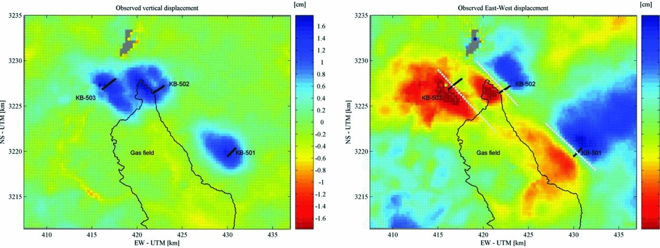
Fig. 32. Left: Vertical displacement, in cm, between July 2004 and May 2008. Right: Horizontal displacements for the same period (eastward motion is blue). Dashed white lines indicate the location of modelled damage zones or tensile fractures. (From Rucci et al., Reference Rucci, Vasco and Novali2013.)
Rinaldi & Rutqvist (Reference Rinaldi and Rutqvist2013) and Rinaldi et al. (Reference Rinaldi, Rutqvist, Finsterle and Liu2017) took the analysis a step further by constructing a coupled model for mechanics and flow for the In Salah field case, and by performing an inversion toward the driving parameters of this model. Based on the outcome of these results they performed a sensitivity analysis to estimate the robustness of the solution and the uncertainty of the parameter estimates.
Lombardia
A stochastic approach was exploited by Zoccarato et al. (Reference Zoccarato, Baù, Ferronato, Gambolati, Alzraiee and Teatini2016) on a gas storage field in Italy. Their approach employed an Ensemble Smoother and had been earlier developed, applied and tested by Baù et al. (Reference Baù, Ferronato, Gambolati, Teatini and Alzraiee2015) on a synthetic reservoir. It further builds on extensive experience with subsidence modelling using finite element models with transversely isotropic elastic behaviour (Janna et al., Reference Janna, Castelletto, Ferronato, Gambolati and Teatini2012) and an earlier non-stochastic calibration of parameters for the same field and using the same data (Teatini et al., Reference Teatini, Castelletto, Ferronato, Gambolati, Janna, Cairo and Bottazzi2011). Zoccarato et al. (Reference Zoccarato, Baù, Ferronato, Gambolati, Alzraiee and Teatini2016) make estimates for the anisotropy ratio and the Poisson ratio, and a parameter is introduced to catch the change in compaction coefficient between the first and subsequent loading cycles. The outcome of the Smoother with different choices of measurement grids is represented in Fig. 33. A clear assimilation is achieved for these parameters, constraining the posterior within narrower bounds when compared to the prior uncertain values. However, there is considerable dependence on the choice of the measurement grid.
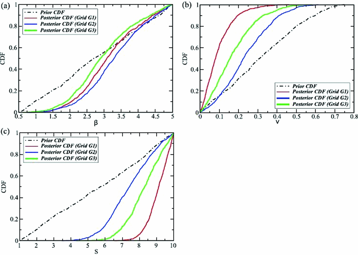
Fig. 33. Results of the Ensemble Smoother working on the Lombardia field: prior (dashed lines) and posterior cumulative density functions for the assimilated parameters. Grids G1, G2, G3 indicate different choices of measurement points.
The Lombardia study makes clear the influence of choices made in the application of the Ensemble Smoother. In Fig. 33 this concerns the choice of measurement grid. The study employed interpolated and projected PS-InSAR data: the G1 grid was a regular grid over the complete area while the G2 and G3 grids were chosen according to the density of persistent scatterers. As the authors indicate, a major challenge is to provide realistic values for the errors in these derived data.
Another challenge in the assimilation process is the proper communication of information between different steps. In the current approach, the pressure field was assumed to be known – it was not part of the assimilation process. This may be a good assumption for the field under study, where ample pressure measurements are available, but in other cases it may not be adequate. In fact, even in cases where the reservoir pressure is well-known there may be uncertainties on the pressure in aquifers connected to the field, which can still have considerable impact on the subsidence pattern.
Bergermeer
The Bergermeer field is a gas field in the northwestern Netherlands which was in production from 1970 to 2007; after that it was converted into a gas storage facility. Surface movement was monitored with optical levelling, but also with PS-InSAR during the later times of its production. Fokker et al. (Reference Fokker, Wassing, van Leijen, Hanssen and Nieuwland2016) used the satellite data to constrain the uncertainties present in the field. The uncertainties considered were the pore pressure in the aquifers adjacent to the field, the compaction coefficient of the reservoir rock and the elastic moduli of the different subsurface layers. The pressure was well-known in the gas-bearing part of the field, thanks to the production wells and elaborate history-matching results.
The data assimilation employed an Ensemble Smoother with Multiple Data Assimilation to handle the nonlinearity of the forward model. The data utilised were the interpreted movements in the line-of-sight of two satellite tracks, which provided two independent sources of data. With the forward model calculating movement in these directions, interpolation and projection to vertical and horizontal movement was unnecessary. The procedure indeed succeeded in a smaller posterior distribution of parameter values as compared to the prior distribution, and in a good match of data and model estimates (Fig. 34).
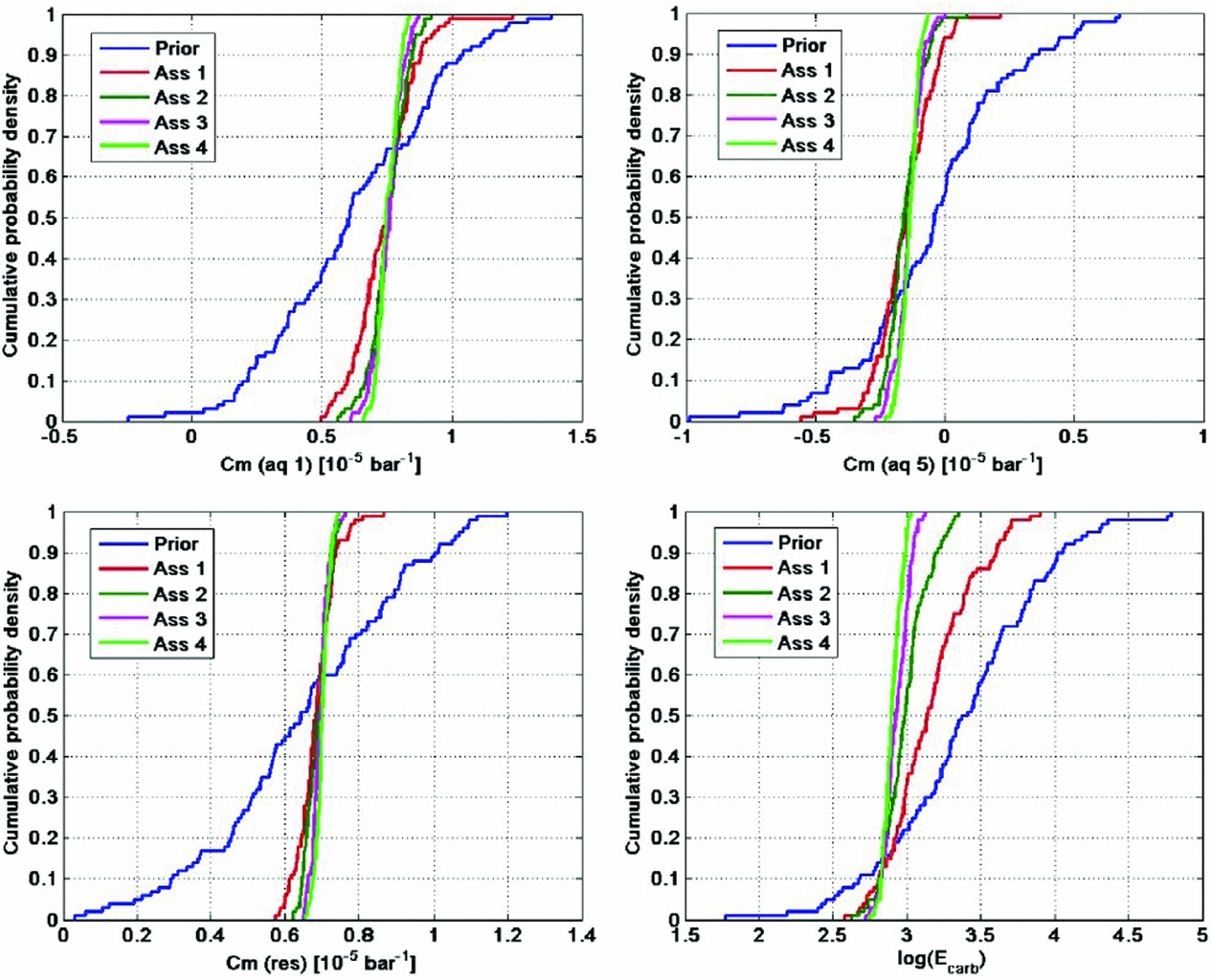
Fig. 34. Assimilation results of the Bergermeer study. The Ensemble Smoother with Multiple Data Assimilation gradually constrains the parameter uncertainty (from Fokker et al., Reference Fokker, Wassing, van Leijen, Hanssen and Nieuwland2016).
In the Bergermeer study the aquifer activity was mimicked using an effective compaction coefficient for these pressure compartments. An improved treatment would be to create multiple reservoir model realisations capturing the uncertainty in aquifer activity. The compaction coefficients were assumed independent of time and pore pressure; especially after the conversion to gas storage an improvement can be made on this.
Pitfalls
The results discussed in the present section elucidate the usefulness of using surface movement data in the process of modelling reservoir processes and understanding the reservoir behaviour. A simple comparison of predicted and measured cross-sections of the subsidence in Lacq hinted at the reservoir structure as an explanatory factor, thus providing insight in the subsurface set-up. However, quantification was not possible. Morton et al. (Reference Morton, Bernier and Barras2006) proposed to employ numerical modelling in their Gulf Coast study; however, the many processes involved made it difficult to provide faithful predictions. An identification of a tensile fracture in InSalah was possible by using more advanced inversion techniques in combination with numerical modelling. The Lombardia and Bergermeer studies showed the strength of combining an in-depth understanding of physical processes, high-quality data and a stochastic inversion or data assimilation approach. An improved understanding upon the use of subsidence data can thus help make subsidence forecasts more precise and more trustworthy. There are, however, some pitfalls.
In the first place, large uncertainties remain connected to the processes involved and to the parameters describing them. The cited literature shows that it is difficult to comprehensively capture all processes. Most of them assume a single deterministic model for the pressure field or for the influence function that propagates compaction to surface movement. Uncertainties need to be acknowledged in an integrated manner. The ensemble methods used in the later studies constitute a useful approach: the spread of possible model concepts and parameter values can be captured in the many model realisations. This also ensures that the prior realisations represent physically sound combinations and that possible correlations between parameters are implemented correctly. Of the various branches of approaches, the Ensemble Smoother with multiple data assimilation seems to be best qualified. It does not suffer from divergence like the particle filter; nonlinearities in the forward model are reasonably captured in the iterative application of the filter; and compared to the EnKF it maintains an internally consistent set of model parameters.
At the same time, there is the uncertainty in the measurements. The process of combining measurements and models to improve subsidence estimates requires a reliable stochastic noise model of the data, including correlations between different measurement points. This should be translated into a full variance–covariance matrix. The treatment of the data, therefore, is of prime importance. Without it, estimates based on a combination of models and measurements cannot be regarded as reliable. We refer to the previous section for a discussion on data treatment.
Even when the stochastic character of data and models is captured, problems can remain. In connection to the data, there can be measurements which are not representative for the process investigated. An example would be the installation of a levelling benchmark on a structure that is sensitive to temperature changes. But also, the models can be inadequate. If a process at work is missed in the modelling, the assimilation can push the parameters of the models to values that are unphysical. Examples are manifold. One can think of nonlinear elasticity; time-dependent compaction creep; unidentified compacting aquifer compartments; viscoelastic behaviour of Zechstein salt caprock. As an example, Hettema et al. (Reference Hettema, Papamichos and Schutjens2002) devoted a study to the delay of start of subsidence after start of production as observed in many fields worldwide. Thus the outcome of an inversion or data assimilation exercise must always be carefully scrutinised for its scientific consistency and its compliance with prior assumptions.
Future subsidence in the Wadden Sea
The aim of this section is to provide estimates of subsidence rates to be expected after 2017. As outlined in the previous sections, an estimate should always be accompanied by a quality measure: a standard deviation or a confidence range of expected numbers. Data from measurements are to be used to constrain the forecasts. In order to assess the impact on the larger Wadden Sea development, the subsidence forecasts need to be formulated in terms of volume rates or areally averaged subsidence rates in the different tidal basins. The tidal basins and their areal extent are given in Table 6 (see Wang et al., Reference Wang, Elias and van der Spek2018). Further, a map showing the tidal basins along with the gas fields and the salt solution caverns is provided in Figure 35. A summary of the subsidence rates as described in the following sections is provided in Table 7. Based on the uncertainty in depleted rock volumes (including the possible depletion of aquifers), the compaction coefficient and the dynamic geomechanical behaviour, we estimate the uncertainty of the average subsidence rates is of the order of 50%. This global number is based on the stochastic study on Ameland, Nes, Moddergat and Lauwersoog reported in Van Thienen-Visser et al. (Reference Van Thienen-Visser, Breunese and Muntendam-Bos2015).
Table 6. Area of tidal basins.
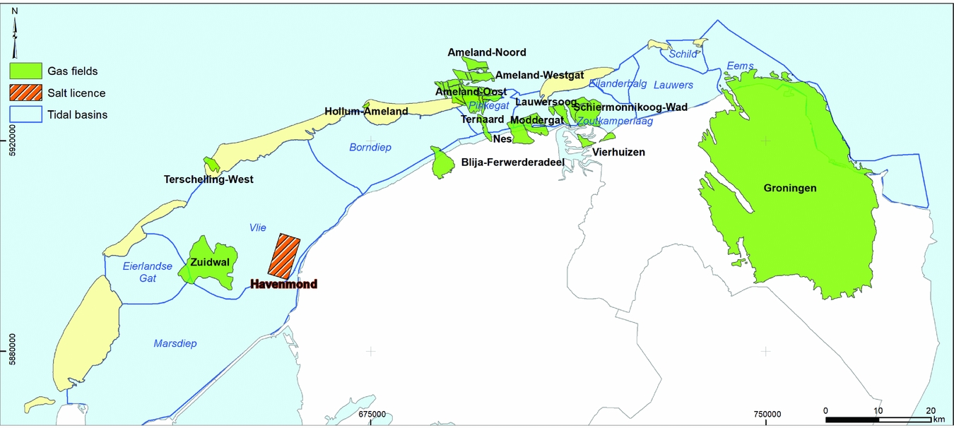
Fig. 35. Map with Wadden Sea tidal basins, relevant gas fields and salt solution mines licence.
Table 7. Volumes of subsidence bowls due to gas extraction in the tidal basins of the Wadden Sea.
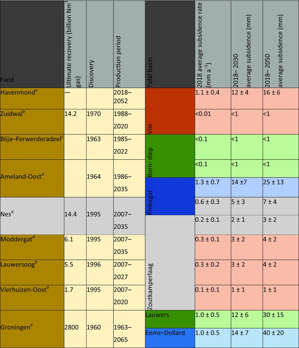
Gas fields
A lot of material is available that addresses the effects of gas production from gas reservoirs in the Wadden Sea. This includes reports from operators or commissioned by them. Such reports cannot be strictly seen as the scientific state of the art: there has not been a peer review process to ensure the scientific value of these documents. Still, many of these reports and production plans contain useful and carefully reviewed information about the Wadden Sea gas fields, and we will use information from them. The Netherlands Oil and Gas portal (www.nlog.nl) has collected a host of relevant information about all Netherlands oil and gas fields. This includes the location of and information on exploration and production wells, applications for production licences, production plans, and production numbers since 2004. Many reports can also be obtained from the website of NAM, the main operator in the area (www.nam.nl).
For the remainder of this section we will first focus on the Zuidwal field (in production since 1988), the Ameland area (in production since 1986) and the Nes, Moddergat, Lauwersoog and Vierhuizen-Oost fields (three fields in production since 2007). An important publication in the scientific realm addressing Ameland, Nes, Moddergat and Lauwersoog is Van Thienen-Visser et al. (Reference Van Thienen-Visser, Breunese and Muntendam-Bos2015). We will therefore give special attention to their work. Then we will consider Groningen, the giant gas field of which a small part is located under the Wadden Sea. Finally, we will briefly discuss two smaller fields contributing to subsidence in the Wadden Sea and a number of stranded fields – discovered gas accumulations which have not (or not yet) been taken into production.
Zuidwal
The Zuidwal field in the western Wadden Sea was discovered in 1970 (Perrot & van der Poel, Reference Perrot, van der Poel, Brooks and Glennie1987). It is a Lower Cretaceous field at 1820–1925m depth, shallower than the other gas fields in the Wadden Sea. Its location is right above a Jurassic volcano, which formed the anticlinal structure. Zuidwal was one of the first gas fields to have horizontal wells used for its development (Celier et al., Reference Celier, Jouault and de Montigny1989; Legris & Nazzal, Reference Legris and Nazzal1989).
Gas production from the Zuidwal field started in 1988. Up to 2015, 14.2 billion Nm3 of gas has been produced. The newest production plan considers a continued production until 2020, up to a maximum cumulative produced volume of 14.3 billion Nm3 of gas.
Subsidence has been measured in a limited number of locations (Rommel, Reference Rommel2004; Vermilion Energy, 2015). Rommel (Reference Rommel2004) made an effort to combine the measurements with model predictions. However, his comparison is only qualitative: the periods of investigation are different and subsidence levels have not been specifically estimated at the measurement points. Also, no analysis of the uncertainty of model predictions and measurements is provided.
A more advanced analysis is provided in the recent production plan (Vermilion Energy, 2015). The pressure and production data of the field allowed determination of the gas volume originally in place and indicate the absence of an active aquifer. Subsidence has been monitored on the production platform during the producing lifetime of the field. Modelling resulted in close bounds on the reservoir pressure. Compaction and subsidence resulting from this pressure reduction was estimated using an analytical model, including a possible subsidence delay. The final estimated maximum subsidence resulting from a calibration of model to data ranged from 10 to 14cm with a subsidence bowl volume of 2.5–5.0 million m3. Two possible interpretations are represented in Fig. 36. The gas remaining to be produced after 2017 is very limited. The remaining subsidence after 2017, however, can vary considerably as a consequence of the delay time modelled. The range of subsidence bowl volumes to be expected after 2017 is not reported in the production plan. We interpret that it will be less than 10% of the total, according to the development of the deepest point represented in Fig. 36. Different physical sources of a subsidence delay can exist, like the inhomogeneous distribution of porosities and associated compaction coefficients and the gradual pore pressure diffusion associated with it, and creep behaviour of the reservoir rock itself.

Fig. 36. Two model scenarios (dashed and solid lines) with different compaction coefficient of the reservoir rock and delay time, calculated for the location on the platform and compared with satellite data (points) (from Vermilion Energy, 2015).
Ameland
The Ameland complex comprises three different fields: Ameland-Oost (discovered in 1964), Ameland Westgat and Ameland-Noord. They are located at a depth of about 3300m and were initially highly overpressured with a gas pressure of 570bar. Production from Ameland-Oost started in 1986. In 2003, production was projected to end in 2018. In 2007, production was extended from newly developed wells and new blocks in the field (NAM, 2003, 2007a,b). The newest production plan of 2011 foresees production until 2035 (NAM, 2011a). Only the Ameland-Oost field contributes to subsidence in the Wadden Sea.
Fig. 35 shows its location, together with the locations of the other fields producing in the area (Nes, Moddergat and the Lauwersoog fields).
The production plan of 2011 (NAM, 2011a) considers uncertainties in reservoir behaviour and the resulting compaction and subsidence. It mentions variations of the permeability, porosity and compaction coefficient, as well as salt creep behaviour and poorly constrained aquifer behaviour. An effort was made to align model results and historical data, and an estimate of the uncertainty of the optimised parameters was given.
The latest yearly update of the monitoring in the Wadden Sea provides the current estimates for subsidence in the Pinkegat and Zoutkamperlaag tidal basins resulting from the gas fields in the area (NAM, 2017c,d). The figures are reproduced in Figs. 37 and 38. The Wadden Sea areally averaged subsidence resulting from production of the Ameland fields is concentrated in the Pinkegat basin and amounts to 1.3mma−1 in 2018, with an estimated total average subsidence of 14mm between 2018 and 2030. From 2030 to 2040, an additional areally averaged 9mm is expected; estimates do not go beyond that date.
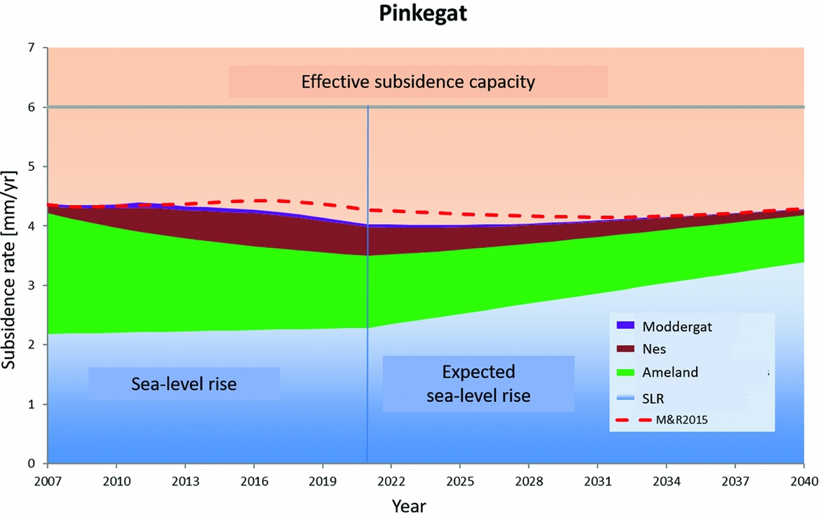
Fig. 37. Expected average subsidence due to production from the Ameland fields (green), Nes (brown) and Moddergat (purple), superposed on the estimated sea-level change in the Pinkegat. The dashed red line is the earlier estimate. The horizontal line at 6mma−1 is the number deemed allowable because of the estimated sand influx. (From NAM, 2017d.)
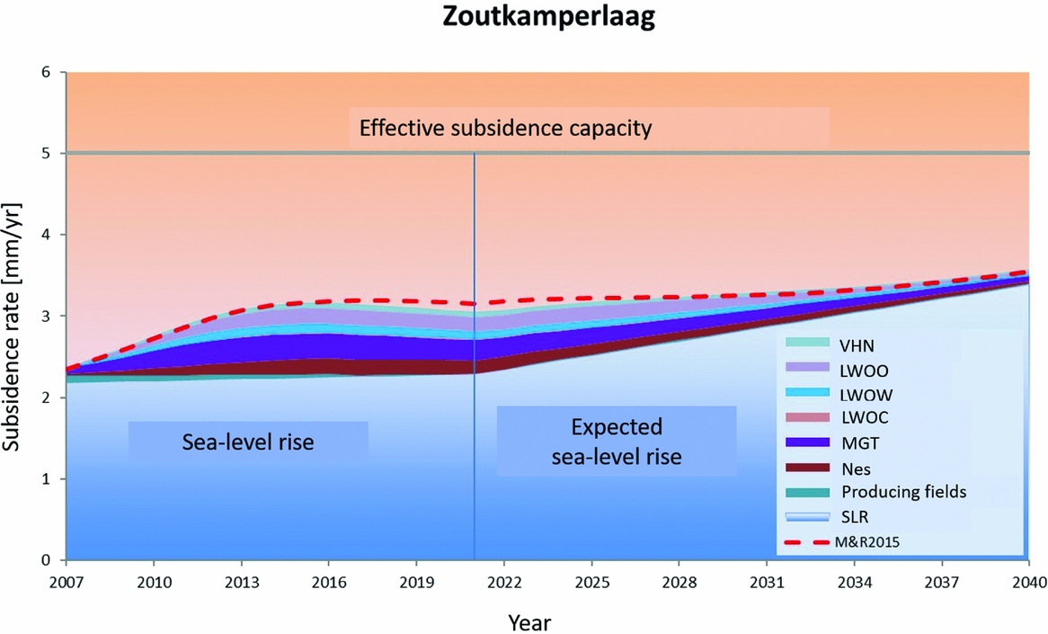
Fig. 38. Expected subsidence from gas fields located in the Zoutkamperlaag (see also description of Figure 5.3) (from NAM, 2017d).
Furthermore, it is not clear at the moment if there will be production beyond 2040. A limited amount of delayed subsidence will result even when production is stopped; we come back to that in thesection ‘Stochastic study of subsidence at Ameland, Nes, Moddergat and Lauwersoog’.
The 2011 extension approval of the production plan for the Wadden Sea area was granted under the condition that NAM would undertake a study aimed at improving the understanding of the long-term predictive capability of subsidence models. Background for this requirement was that the Ameland field displayed a continuing surface subsidence at the deepest point, even after pressure depletion had slowed considerably (see e.g. Houtenbos, Reference Houtenbos2017). This behaviour was not well understood and required the introduction of a time- (and/or rate-)dependent mapping function between reservoir pressure change and subsidence in order to explain the mismatch between model predictions and survey measurements. We consider the use of an unidentified diffusion process in the model for subsidence prediction as unsatisfactory.
The results of the first long-term subsidence study (LTS-1) were reported in 2015 (NAM, 2015). The conclusions were that indeed the time-dependent subsidence effect is real, and not an artefact of noise or uncertainty in the data. Physical processes responsible for this behaviour were identified: delayed compaction of the reservoir rock, salt flow of the caprock, ongoing delayed depletion after production, including aquifers) (NAM, 2016a). It was concluded that neither of the identified physical processes can provide a sufficient explanation for the observed subsidence when considered in isolation.
The scientific steering committee, established to provide guidance and advice on the outcome of the LTS study, recommended: (i) testing of various hypotheses on the Ameland field case and (ii) further research on different aspects of time-dependent subsidence, including field-scale numerical modelling to study the combined effect of different physical processes contributing to the time-dependent subsidence behaviour (Wadden Academy, 2016). Better handling of subsidence measurement data was suggested to take into account the correlations between subsidence numbers estimated from them, and an improved stochastic handling of models was suggested to capture the uncertainty of the models and the model parameters. The latter recommendations had not yet been implemented on the Wadden Sea fields. Following recommendation (i) of the scientific steering committee, a second phase of the LTS study started in 2016 on the Ameland fields (NAM, 2017a,b). The Netherlands States Supervision of the Mines identified a number of issues in the results of this study, and NAM is currently working on an update.
Since the start of production from the Ameland field, a commission has been facilitating monitoring effects of subsidence on Ameland island. The research encompasses the morphology of the island, and the effect of subsidence on the ecology – mainly birds and vegetation – both on the island and on the Wadden Sea area around it. A comprehensive report was recently presented (De Vlas., Reference De Vlas2017).
Below in the section on ‘Stochastic study of subsidence at Ameland, Nes, Moddergat and Lauwersoog’, we provide an estimate of the contributions from Ameland, Nes, Moddergat and Lauwersoog to the average subsidence rates in the tidal basins Pinkegat and Zoutkamperlaag.
Nes, Moddergat, Lauwersoog, Vierhuizen-Oost
The fields Nes, Moddergat, Lauwersoog and Vierhuizen-Oost were discovered in the mid-1990s. They are located at the coast of the mainland, southeast of Ameland and southwest of Schiermonnikoog; we refer to Fig. 35 for a location map. The fields were encountered as overpressured like Ameland. Production started in 2007. Production until December 2016 has been in total 8.6, 3.8, 3.3 and 1.5 billion Nm3 respectively for these fields, with an estimated additional production from 2017 onwards of 5.7, 2.6, 2.3 and 0.2 billion Nm3 respectively (NAM, 2017d).
NAM (2011b) provided an estimate for the future subsidence. In the analysis, a number of modelling choices have been made. These include the choice of (1) compaction coefficient, (2) a delay of the onset of subsidence after the start of pressure depletion, (3) a delay of cessation of subsidence upon decrease of depletion, (4) the extent of the connected aquifer of which the pressure is also depleting, and (5) the effect of salt creep. For the delay time, a calibration was used that was derived using measurements above similar fields: Anjum, Ezumazijl, Metslawier. These measurements were also used to calibrate the salt creep behaviour. In view of this we consider the values of the predicted subsidence to be subject to considerable uncertainty.
In NAM's last yearly update of the subsidence monitoring (NAM, 2017c,d), the average subsidence rate in the Pinkegat tidal basin due to the Nes field was about 0.6mma−1. A total average contribution of 5mm was calculated for 2030 and another 2mm from 2030 to the end of production. For the Zoutkamperlaag tidal basin the current average subsidence is about 1mma−1. The contributions from Nes, Moddergat, Lauwersoog and Vierhuizen-Oost are 0.2, 0.3, 0.3 and 0.1mma−1 in 2018. Based on this distribution and the total expected subsidence in 2030 (8.6mm), we estimate contributions of 1.9, 2.9, 3.0 and 0.7mm; for 2030 to the end of production we derive 0.7, 1.0, 1.0 and 0.2mm.
The NAM report on dynamic reservoir modelling of Wadden fields for subsidence (Tichler, Reference Tichler2016) provides an updated analysis and more detail on the geology and the reservoir dynamics.
Stochastic study of subsidence at Ameland, Nes, Moddergat and Lauwersoog
Van Thienen-Visser et al. (Reference Van Thienen-Visser, Breunese and Muntendam-Bos2015) provide a stochastic analysis of the combined subsidence volume rates to be expected from the fields Ameland, Nes, Moddergat and Lauwersoog (Fig. 39). The numbers agree with those given in the previous sections. In addition to the studies by NAM (2017c,d) described in the previous sections, Van Thienen-Visser et al. (Reference Van Thienen-Visser, Breunese and Muntendam-Bos2015) provide a time-dependent subsidence load (average subsidence rate in the tidal basin) in the two affected basins based on a stochastic analysis.
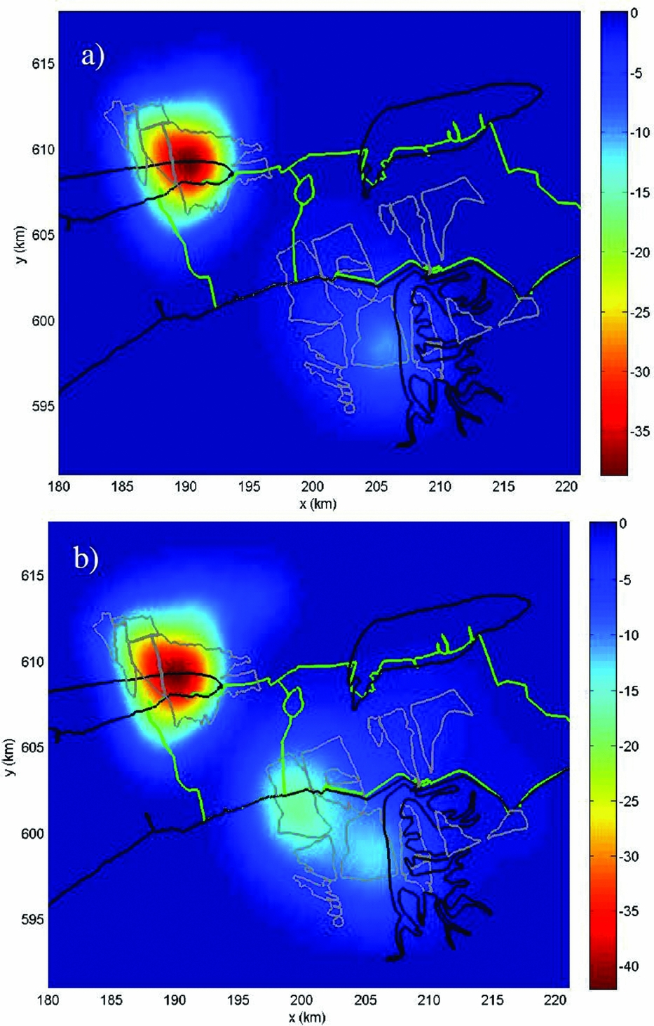
Fig. 39. (a) Subsidence (in cm) in 2011, modelled using a best fit to the measured subsidence. (b) Prognosis of subsidence in 2050. Also indicated are the coastlines (in black), the gas field contours (in grey) and the tidal basins of Pinkegat and Zoutkamperlaag (in green). (From Van Thienen-Visser et al., Reference Van Thienen-Visser, Breunese and Muntendam-Bos2015.)
Fig. 40. The subsidence load for the tidal basins Pinkegat (a) and Zoutkamperlaag (b). The black part indicates the period in which the history match was created; the grey part indicates model forecasts. (From Van Thienen-Visser et al., Reference Van Thienen-Visser, Breunese and Muntendam-Bos2015.)
To come to a stochastic estimate of the subsidence load, Van Thienen-Visser et al. (Reference Van Thienen-Visser, Breunese and Muntendam-Bos2015) created a large number of scenarios. The uncertainty in the reservoir dynamics was captured by creating several history-matched reservoir models. The uncertainties considered included the aquifer activity and the amount of producible gas. The match ensured that the observed reservoir well pressures were consistent with the subsurface model calculations.
Geomechanical models were built on the reservoir model realisations, with different geomechanical parameter realisations. All possible combinations of models together resulted in more than 85,000 variants of the surface-averaged subsidence rate. These numbers are supposed to envelop the consequence of the uncertainty in dynamic and geomechanical models for the subsidence estimates. Finally, the load for the tidal basins was calculated as a temporal moving average of the surface-averaged subsidence rate for periods of 19 years.
Results for the two tidal basins are reproduced in Fig. 40. In Pinkegat, the load starts in the late 1970s due to the start of production of Ameland. The Zoutkamperlaag load follows later, as a result from the other fields. After 2020, all loads decrease gradually until they disappear around the year 2050 due to the cessation of production.
Compared to NAM's results (NAM, 2017c,d), the results of Van Thienen-Visser et al. (Reference Van Thienen-Visser, Breunese and Muntendam-Bos2015) for the Pinkegat tidal basin are somewhat smaller (1–2mma−1 vs 2mma−1); those for the Zoutkamperlaag basin are in line with NAM's results (both around 1mma−1). In Table 7 we report the more conservative NAM numbers. Between 2040 and 2050 we use the high estimate of the range of Van Thienen-Visser et al., resulting in a total of 2.5mm subsidence in the Pinkegat basin during that period, attributed to Ameland-Oost.
For Zoutkamperlaag, the total estimates of Van Thienen-Visser et al. (Reference Van Thienen-Visser, Breunese and Muntendam-Bos2015) and NAM (2017c,d) are consistent: around 1mma−1 in 2018.
Groningen
The Groningen gas field, discovered in 1959 and in production since 1963, is the largest gas field in western Europe. It is mainly located onshore, but a small part of the field is located below the Wadden Sea and the Eems–Dollard. Subsidence has been monitored since the start of production. Fig. 41 reproduces the measured and modelled subsidence until 2013 on top of a map of the gas field (NAM, 2016b). For the present paper, only the part of subsidence in the Wadden Sea area caused by gas extraction from the Groningen field is relevant. This was not separately reported, therefore we have estimated subsidence bowl volumes from the production plan and the associated addendum (NAM, 2016b,c). The subsidence predictions for the two models that they used are reproduced in Fig. 42. A later inversion study by Van der Wal & Van Eijs (Reference Van der Wal and van Eijs2016) did not result in significant changes of the estimates.
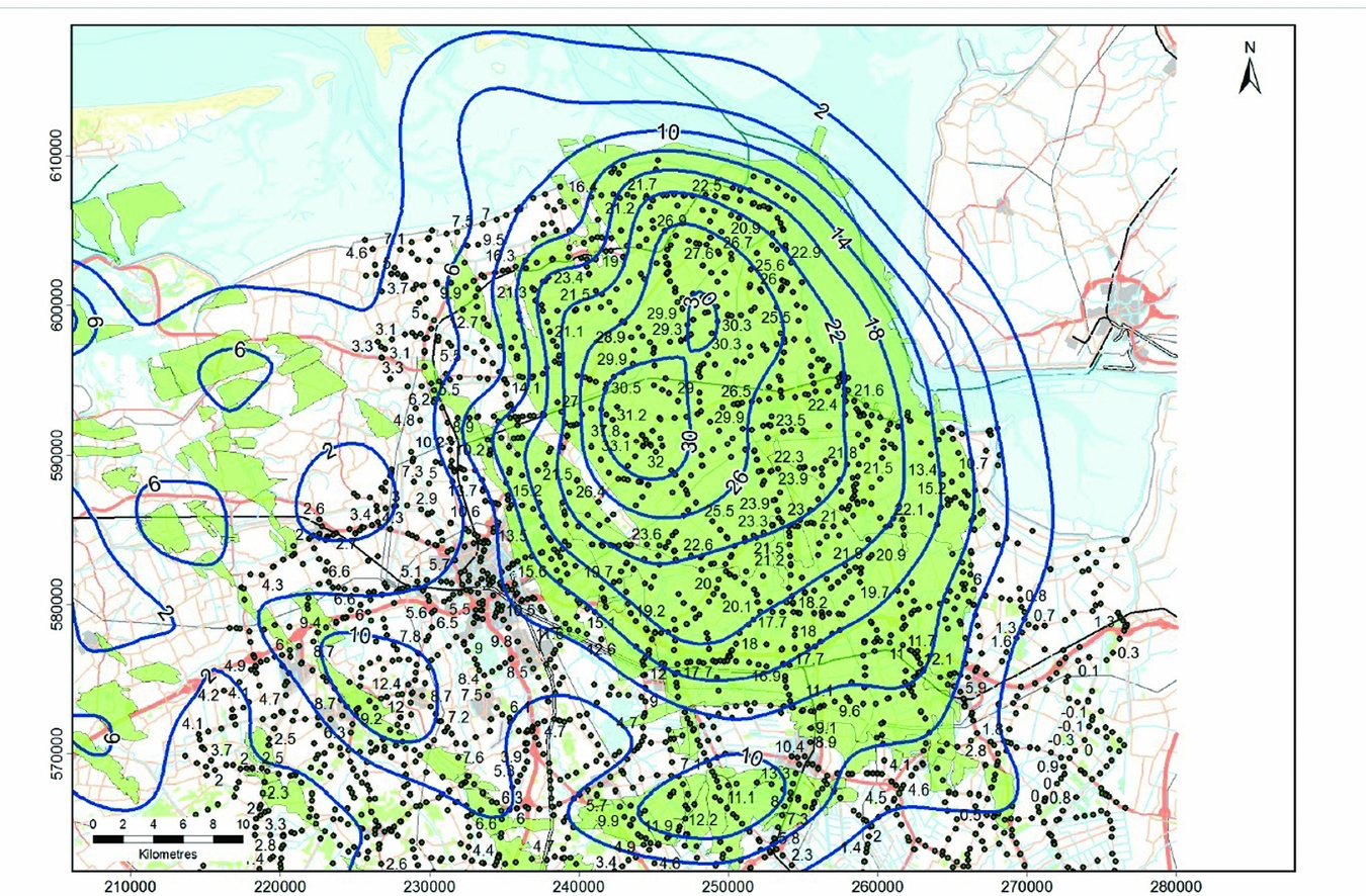
Fig. 41. Subsidence measured from 1972 to 2013, and contour lines of subsidence (numbers in cm) as modelled resulting from gas production in Groningen and neighbouring fields (NAM, 2016b).
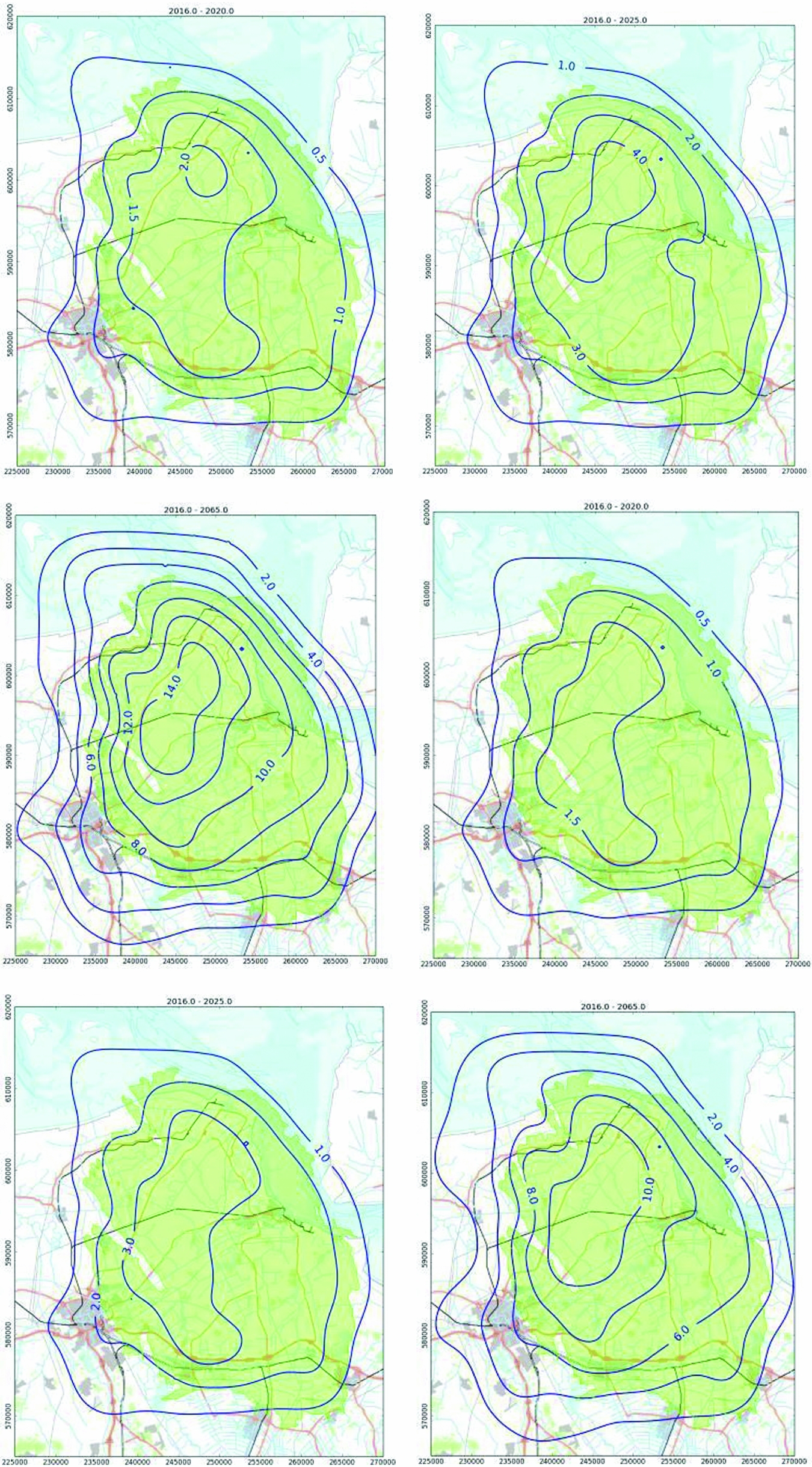
Fig. 42. Estimated subsidence due to production from the Groningen gas field. Contour lines indicated in cm. Top row: Time Decay model. Bottom row: RTCiM model. Left: 2016–2020. Middle: 2016–2025. Right: 2016–2065. (From NAM, 2016c.)
We follow the more probable lower production scenario of NAM (27 billion m3a−1 annual from 2017; see NAM, 2016c). A global integration of the subsidence bowl over the tidal areas yields a total of 3.5 and 18 million m3 as volumes of subsidence bowls in the tidal basins Lauwers and Eems, respectively, between 2018 and the end of production; 1.5 and 6 million m3 between 2018 and 2030 (extrapolating the numbers for 2017–2025). Subsidence in the Schild tidal basin is negligible. The average subsidence rates in 2018 in both basins amount to approximately 1mma−1. These numbers clearly are quite crude zeroth-order calculations of which we estimate the quality to be in the order of 50% accuracy.
Fokker & Van Thienen-Visser (Reference Fokker and Van Thienen-Visser2016) published a study in which they attempted to integrate the knowledge on compaction and subsidence available for the Groningen gas field. They performed an inversion exercise on the available levelling data in the area, utilising the complete information available on the geology and the pressure development in the field. Double differences were used instead of the often-used single differences, which is a major improvement when in the employment of single differences only the variances are known.
The study resulted in some areas of increased or reduced compaction relative to the prior compaction field. These areas correspond to areas of possible discrepancies in porosities and aquifer activity from another study. The study did not, however, provide explicit estimates of forecasted subsidence and its confidence bounds in the Wadden Sea.
Blija-Ferwerderadeel
Blijja-Ferwerderadeel is partly located below the Wadden Sea, partly below land, at a depth of about 2600m. The field was discovered in 1963 and has been in production since 1985.
Abandonment is expected in 2022 or soon after. According to the production plan, the resulting subsidence will be smaller than 2cm at the deepest point and not measurable (NAM 2007c). The volume of the part of the subsidence bowl in the Wadden Sea is negligible with respect to the volumes resulting from other fields and the uncertainties in them.
Stranded fields
A number of fields in the Wadden Sea area have been discovered but have not or not yet been taken into production. We briefly summarise them here, and provide an estimate of the subsidence bowl volume and rates in the Wadden Sea in case they would be produced. The information can be found at www.nlog.nl/en/stranded-fields. We have not included subsidence estimates in Table 7, as the production of these fields is still uncertain. Further, prospects that have not yet been drilled are not included in the present section.
Ternaard
The Ternaard field was discovered in 1991 but has not yet been taken into production (NAM, 2017e). It is a structure at a depth of about 3500m, with an estimated total recoverable volume of gas of 4 billion Nm3. The initial reservoir pressure is 525bar, which is overpressured similarly to Ameland. With compaction coefficients similar to those in Ameland we would expect 1–3 million m3 subsidence bowl volumes in the Wadden Sea area, mainly in the Pinkegat tidal basin. If the field were to be produced in 15 years, this would imply an average subsidence rate of 2.0mma−1. These numbers, however, are subject to considerable uncertainty, both because of the compaction coefficient and the precise amount of recoverable gas.
Schiermonnikoog-Wad
The Schiermonnikoog-Wad gas field was discovered in 1996 by NAM by well Lauwersoog-01 (LWO-01). The primary target of the well was gas in the Slochteren Formation of the Lauwersoog prospect. However, the Lauwersoog-01 well also showed gas in the shallower Bunter formation, which indicated the Schiermonnikoog-Wad field. An estimate of the amount of gas is not available. It is not expected that this field will be produced, as the operator NAM has not pursued the drilling of an appraisal well.
Hollum-Ameland
The Hollum-Ameland field is situated west of the Ameland-East field. It was discovered in 1964. Technically recoverable volumes are less than 0.5 billion Nm3; associated subsidence has not been calculated, but can be assumed to be negligible in view of its uncertainty and the effect and uncertainty of other fields.
Terschelling-West
The Terschelling-West field was discovered in 1989 onshore of Terschelling island. It has a technically recoverable volume of less than 1.0 billion Nm3. The gas is of poor quality.
Expected subsidence would mainly be located onshore; the effect on the Wadden Sea would be negligible.
Salt solution mining in Havenmond
Since 1995, Frisia Zout B.V. (Frisia) has produced salt by solution mining in the Barradeel region near Harlingen. Frisia plans to move production to the Havenmond production licence in the Wadden Sea as from 2018. Salt is produced by solution mining in squeeze mode, thereby retaining a balance between decrease of the cavern volume through convergence and increase by salt dissolution and brine production. Much experience has been gained during the past 20+ years of deep salt solution mining in Barraddeel, which is used to predict future subsidence in the Havenmond region in the Wadden Sea.
In Barradeel, salt has been leached from two caverns in the Barradeel concession (Frisia Zout, 2003b) and also from two caverns in the Barradeel II concession (Frisia Zout 2003a, 2011). The extraction licences are issued under the condition that the maximum subsidence due to salt extraction stays within 35cm in the Barradeel and 30cm in the Barradeel II concession. At the end of 2016, the actual maximum subsidence was close to the subsidence limits prescribed by the regulatory authorities: ~32.5cm in the Barradeel and ~26cm in the Barradeel II (www.nlog.nl). After reaching the limits of current licences in a few years’ time Frisia plans to continue its economic activity by extracting salt from the new Havenmond production licence.
In the Havenmond project, deviated wells will be drilled from the Frisia salt plant in Harlingen to the target locations below the Wadden Sea at a depth of about 3000m (Frisia Zout, 2012). Four new caverns are planned to be leached in succession with a time lag of 5–10 years. Each cavern will operate for about 15 years. The caverns are located 3–3.5km off the coast of Harlingen in the Havenmond concession (Fig. 43). The caverns are positioned as far as technically possible from the coastline, given the limitations of the present well-drilling technology (~3750m maximum horizontal reach from the drilling location), to minimise the impact of subsidence on the dikes. Mutual distance between the caverns is planned at 500–1000m, which implies the superposition of the effect of the four subsidence bowls.
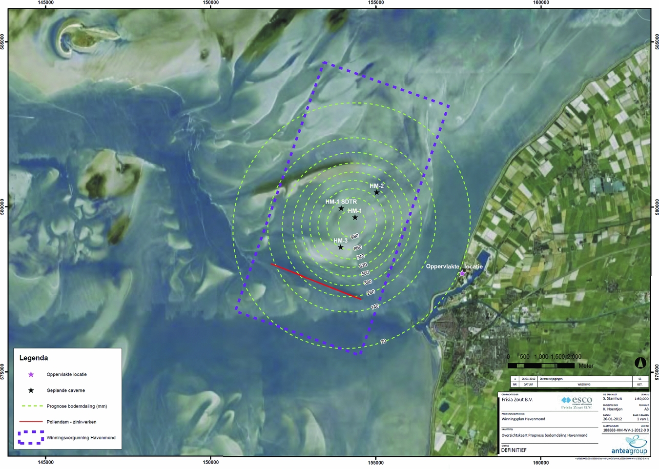
Fig. 43. Forecasted maximum subsidence 2015–2052 due to salt production from Havenmond (contours in mm) (from Frisia Zout, 2012). Maximum subsidence amounts 103cm.
Subsidence forecasting was done using the analytical approach described in the section ’Optical levelling’ above, assuming a Gaussian shape for the subsidence bowl (Frisia Zout, 2012). The predicted subsidence at the deepest point at the end of salt extraction in 2052 amounts to 103cm, while the subsidence at the coast is estimated at ~2cm). The subsidence is calculated assuming that each cavern has a volume of 1 million m3; it will produce 8 million tons of salt and create a subsidence bowl of Gaussian shape (cf. eqn 6) with a maximum depth of 27.5cm. The subsurface volume of the produced salt from a single cavern is about 3.6 million m3; with the remaining 1 million m3 of shut-in volume after production stops, the convergence volume is 2.6 million m3. Four caverns sum up to 10.4 million m3, or an average subsidence in the Vlie tidal basin of 16mm. Different production scenarios yield a maximum subsidence ranging from 1 to 1.5m (Fig. 44) and an average value of 14–20mm in the Vlie tidal basin. The production scenarios consider variations in the annual salt extraction (average 1.35, minimum 0.82 and maximum 1.56Mta−1).
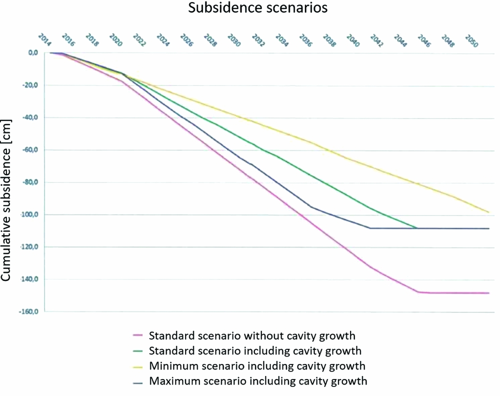
Fig. 44. Forecasted evolution of maximum subsidence 2015–2052 due to salt production from Havenmond for four scenarios (from Frisia Zout, 2012).
Subsidence predictions for Havenmond are based on the experience and best practices proven to lead to reliable subsidence predictions at Barradeel. A similar conclusion was drawn in a position paper specifically dedicated to salt solution mining in the Wadden Sea recently issued by the Waddenacademie (Hulscher et al., Reference Hulscher, Meire, Rienstra and Urai2016). As in gas production situations, there is a continuous requirement for sonar monitoring to check the salt cavern dynamics and for subsidence monitoring to check the subsidence forecasts.
After cavern abandonment, a delayed subsidence can still occur due to further squeeze of the cavern. Continued convergence and brine thermal expansion can increase the brine pressure and facilitate loss of brine by permeation to surrounding and overlying layers. This permeation process, however, will be much slower than the immediate squeeze during production and will terminate when brine outflow balances cavern convergence rate (Bérest et al., Reference Bérest, Brouard and Mehdi2005). The reason behind the rate decrease is that the driving force for the convergence, equal to the difference between the in situ stress and the brine pressure, reduces dramatically after shut-in. The solution-mined caverns at Barradeel (and future caverns at Havenmond) are expected to follow the same pattern after abandonment, as discussed by Duquesnoy (Reference Duquesnoy2017).
The effects on subsidence of the fluid migration due to permeation are expected to be marginal, with the possibility of some bowl widening (Van Heekeren et al., Reference Van Heekeren, Bakker, Duquesnoy, de Ruiter and Mulder2009).
Gaps analysis and way forward
The knowledge accumulated so far gives rise to the identification of gaps and possible solutions or improvements of the current practice. For the convenience of the reader, we summarise the discussion in Table 8.
Table 8. Gaps, issues, and associated recommendations.
Measurements
For the Wadden Sea region it is quite difficult to obtain measurements of the movement of the Pleistocene layers as a result of gas production and salt mining which are accurate and have sufficient spatial and temporal sampling. The surface of the tidal flats is continuously reshaped because of the dynamics of the morphology, and movements within shallow layers cannot be independently assessed. Therefore, measurements must either rely on deeper founded benchmarks, or shallow and morphological changes should be measured independently. In the Wadden Sea, only campaign-style GPS is currently available. GPS benchmarks have been installed since 2007 on platforms, on founded points in the Wadden Sea and on a few onshore locations. For a proper interpretation it is important that these points are evaluated together with points onshore, from both levelling and InSAR. Only a fully integrated treatment has a chance of improving understanding of the subsurface behaviour.
The characterisation of the subsidence development in the Wadden Sea further requires the installation of a sufficiently dense network of GPS benchmarks, which is subsequently surveyed sufficiently often. Especially for the area below the possibly active aquifer connected to the Ameland-Oost gas field it would be helpful to install additional points. New points may also be required above fields that could possibly be developed in the future, like Ternaard.
The treatment of subsidence measurements has attracted considerable attention (Houtenbos, Reference Houtenbos2011). One important lesson is that geodetic measurements cannot and should not be seen as completely independent of the models used to describe the physics. It should be acknowledged that meaningful measurements are implicitly impossible without prior information on the expected deformation signal. Therefore, instead of suggesting that decoupling should be strived for, it is important to explicitly formulate and document all relevant prior knowledge that is used to design the measurement network, choose the measurement methods, perform the actual surveying and process the survey data. This can be referred to as contextual information.
InSAR measurements are currently being performed by several independent satellites; the acquired data are readily available, and it is the only technique that covers all areas affected by mining in the northern Netherlands in an integrated way. Therefore it is advantageous to use this technique for all land sites, including the Wadden Islands. Some of the data-processing methods should be fine-tuned for the island character of some of the sites. To enable the coupling of the different techniques, integrated reference stations (IRS) should be deployed, similar to the ones currently installed over the Groningen site.
Models
Understanding the cause of subsidence in terms of subsurface processes is impossible without the help of models. Faithful forward models are thus a prerequisite for any subsidence study in which a quantitative insight on the cause is pursued. Analytic and semi-analytic models run fast and can be used in stochastic studies; they may, however, miss important characteristics, like subsurface heterogeneity or complex constitutive behaviour. Such issues can often be captured in numerical models, but these require more computing time and can therefore not easily be used in stochastic methods. They may, however, serve as a reference for the fast models. And indeed, all models employ parameters that may depend on the specific material composition and on external factors like temperature, stress, pore pressure and pore fluid composition. The large variability and uncertainty of these parameters requires a stochastic treatment: we must incorporate the limitation of our knowledge as an uncertainty on the parameters and the models. This is analogous to what is routinely done in weather forecasting.
Model improvement in itself is not a goal. However, it is necessary to improve the understanding of the subsurface and the associated quality of subsidence forecasts. For the purpose defined in this document, the first issue seems to be the incorporation of complex geology and physics in fast models. This enables their use in ensemble methods for data assimilation. A second issue is the frequent discrepancy between the shape of measured and modelled subsidence bowls. The physics that control these shapes must be carefully scrutinised. This includes the basic assumption of the nucleus-of-strain approach and the effect of overburden salt layers. A third issue is the delay and the nonlinear relationship that is regularly observed between reservoir pressure depletion and surface subsidence. This delay can be related to nonlinear compaction and creep of the depleted reservoir or to elasto-visco-plastic behaviour of overburden salt, or both. Much knowledge is still to be gained with laboratory research in combination with constitutive modelling of these materials and high-rate geodetic measurements. The delay can also be related to delayed depletion of low-permeability aquifers; in that case the focus should be on the reservoir behaviour. The signature of the subsidence pattern in time and space can help quantify the various contributions to the subsidence. Finally, the models used may not cover all physics at work. There may, for instance, be processes (e.g. compaction) of shallow Pleistocene layers triggered by the morphological dynamics that are not modelled. Onshore, there may be compaction or decompaction induced by groundwater level changes. It can be hard to quantify these processes. A qualitative assessment, however, may shed some light on the magnitude of the effect, which can then possibly be incorporated as idealisation noise in the measurements. This needs, however, to be further elaborated.
Inversion or data assimilation technology
An integrated approach is thus warranted. Starting from existing knowledge of the behaviour of the subsurface and the driving parameters, modelled surface movement numbers can be obtained. The uncertainty of the processes and the parameters should be translated to a range of model outcomes. Geodetic measurements can then be used to constrain the parameters in these models. Key in such a treatment is to properly account for the uncertainty in model parameters and data, including correlations. The combined results can be used to obtain improved forecasts, which can be evaluated later against geodetic measurements that were not yet available at the time of the model study. Such an assessment critically requires a quality measure of the forecasts.
A fruitful way to set up such an integrated treatment is with an ensemble of model realisations that span the uncertainty of the prior knowledge. Data assimilation should be used to constrain that uncertainty, by making an ensemble of predictions that shows smaller variability. The full loop is schematically demonstrated in Fig. 45.
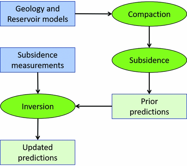
Fig. 45. Compaction and subsidence modelling, and inversion workflow (from Van-Thienen-Visser & Fokker, Reference Van Thienen-Visser and Fokker2017).
Data assimilation can be performed in many ways. Approaches that have been mentioned in the section ‘Combining models and measurements’ are Ensemble Kalman Filter, Ensemble Smoother and Particle Filter. The choice of the optimum method is not straightforward, and different choices come with different trade-offs. Examples are ensemble collapse, when the spread of forecasts reduces more than is justified by the uncertainty of the data; or adjustment of the parameters outside physically acceptable limits. A study that puts these methods in the context of subsidence forecasting for the Wadden Sea and that makes quantitative comparisons between different approaches would be appropriate.
Requirements for quantitative interpretation and forecasting
The quality of the geodetic and contextual data is critical input in the inversion or data assimilation loop. First, the data interpretation needs to be performed very carefully. This includes the careful treatment of raw data to identify outliers, identification errors and disturbances. For the data surviving these tests, the quality description is key input. Data assimilation requires a full description of the quality in the form of uncertainty and correlations: using only variances or standard deviations in the data assimilation is incorrect. The data quality should be quantified in the form of a so-called variance–covariance matrix.
Even though GPS data are less precise in vertical deformation than levelling data, they have an important additional feature, as horizontal movements are also measured. These horizontal movements are not the goal of the kind of studies discussed here, because they do not contribute to the volume of the subsidence bowl. However, they are instrumental in the data assimilation because they provide an independent additional constraint.
Forecasts
It has already been mentioned that forecasts must always be accompanied by a quality measure. Only then can the forecasts later be judged against future geodetic measurements. Model forecasts are often based on a train of modelling and interpretation efforts. The uncertainty and correlations in the various steps should then be faithfully propagated through the various stages. This will circumvent the accumulation of ‘worst cases’ in different steps that can lead to physically unrealistic numbers. This reasoning also applies to the full present report. Expected subsidence levels given in the present section and used in the other parts of this report must include their uncertainty range.


 Open access