


1. Introduction
An aging population presents various challenges for society. One of the most prominent challenges is to cope with the increasing need for elderly care. Households use both paid and unpaid care to meet this need. In 2015, around 12% of people older than 65 received some care from care facilities while at least 23% of people in this age group need regular help, so facilities that provide formal care, such as nursing homes, are not sufficient in meeting all the needs.Footnote 1 In fact, unpaid and family caregivers provide a significant portion of the overall care for elders. In 2015, 41.3 million people in the United States provided unpaid care to their elder relatives, and a fifth of them gave care on a daily basis.Footnote 2 To capture the full scope of the implications of caregiving in an aging population, we need to understand how different households choose to meet their elder care needs.
Adult children stand out as a group when we look at who provide elder care. We find that they are, by far, the largest group in unpaid caregivers: based on the 2015 National Health and Aging Trends Study (NHATS), of those who cared for people over 65 without pay, 56% are adult children with 38% being daughters. Their average age is 57, so many of them would face the potential conflict of caregiving and employment. While the existing empirical literature suggests that caregiving may negatively affect labor supply (e.g. Lilly et al. Reference Lilly, Laporte and Coyte2007), only 13% of adult daughters claimed that caregiving has kept them from work, though half of them work as well as providing a non-negligible amount of care. This shows that the tradeoff between caregiving and employment is relatively nuanced for most of them. In addition, we find that adult children provide less care (and money) to parents who are financially better off. This suggests that the transfers from adult children to elder parents are at least partially driven by the needs of the parents. We refer to this as a “need-based altruistic” motive for parental care. Parents use their own resources to take care of themselves, and when they cannot fulfill all their needs, adult children step in.
We propose a static model with adult children and aged parents to study the effect of elder care responsibilities. The focus is on the adult children generation, particularly adult daughters. Agents in our model are heterogeneous in labor productivity, spousal income, and whether they have parental need. All households face a probability of receiving a parental health shock. For the shocked households, a small fraction of them are eligible for a mean-tested program, similar to Medicaid, which uses public funding to cover all elderly care need in the households. For the remaining households, parents will use a fixed fraction of their assets to purchase care services, and when that is not enough to meet their needs, adult children will fill in the gap using informal care with own time and money. We set up and estimate a CES production function for the informal care provided by children, who choose a combination of time and monetary inputs based on the opportunity cost of their time, input productivity, and input substitutability. Our estimates of the care production function show that while time and monetary spending are quite substitutable in producing care, caring with own time is more effective in meeting parental care needs.
There are two production sectors in the economy: consumption goods and care services. Women choose which sector to work in based on their prospective wages. Care price and care wage are determined endogenously by market-clearing conditions. We calibrate the model using data from the Health and Retirement Study (HRS), the National Health and Aging Trends Study(NHATS)/ National Study of Caregiving (NSOC), and the American Community Survey (ACS). In addition to labor market statistics, we match three moments about parental care: the average time daughters spend caring for parents, daughter’s wage elasticity to care time, and the percentage of informal care usage. The wage eligibility setting is disciplined by the actual Medicaid recipiency rate for the age group of our interest.
The calibrated benchmark model shows that adult children with an income in the middle range face the largest parental care need, as Medicaid covers the low-wage households and the high-wage households are able to purchase more formal care. To fulfill the care need, most children exclusively use own time to provide care while only the highest-wage earners spend money in caregiving. Caregiving has a small effect on adult daughters’ work hours (a decrease of 0.2 hours per week), which is consistent with the survey results from the 2015 National Study of Caregiving that most children do not report that caring for parents keeps them from work. Our model replicates a modest effect of caregiving on employment rate found in the same data. Caregivers are less likely to be employed, with an employment rate of 47% relative to the overall female employment rate of 57%.
We then use the model to simulate care decisions in an aging population structure and explore the roles of government interventions. Population aging will increase the frequency and intensity of parental care need through a longer life expectancy and a higher dependency ratio. We adjust the model setting to reflect the population structure in 2060. Without intervention, the increased demand for care services will push up the cost of formal care and expand the care sector. Non-care sector shrinks by 1.8% due to extra caregiving time crowding out work hours. The health shock from the aged population generates, on average, an extra 63.4% welfare loss for the adult children households compared to the benchmark. To mitigate this increased impact of caregiving, we propose three government interventions and study their impacts. The first one is a subsidy that lowers the out-of-pocket price of formal care. This program causes a shift from informal care to formal care, leading to a higher care price and larger care sector. We also find the main beneficiaries of this program are the high-wage adult children as their households purchase most of the care in the market. We then consider a Medicaid expansion program by raising the income limit for coverage eligibility. While having a similar effect on care provision overall as the subsidy, Medicaid expansion, by design, causes most welfare improvements for the poor. With the intention to directly benefit adult children, we consider a caregiver allowance that is distributed based on caregiving time.Footnote 3 Our results show that this program has little effect on care arrangement, and the welfare gain to adult children caregivers is also minimal.
This paper belongs to the literature on elderly care in general. Chandra et al. (Reference Chandra, Coile and Mommaerts2023) provide a thorough overview on care provision in the USA and the economic implications of Alzheimer’s disease. They point out Medicaid program bears a heavy weight for total care costs, and the remaining costs fall on household savings, families who provide care, and the least amount is covered by private insurance. Reaves and Musumeci (Reference Reaves and Musumeci2015) and Kopecky and Koreshkova (Reference Kopecky and Koreshkova2014) both provide evidence that a large percentage of formal care expenditure is covered by public funding. Our inclusion of a means-tested government program similar to Medicaid aims to reflect this observation, and the calibrated model generates an economy where 60% of formal care is purchased through the government program. Barczyk and Kredler (Reference Barczyk and Kredler2019) show another important pattern of elderly care arrangement that most households rely heavily on informal care. Using the HRS data, they found 76% of the care cases are either only informal care or a mix of informal and formal care, relative to the 5% of formal home care and the 19% of nursing home care. This finding echoes with the motivation and the main focus of our study. Most households are not covered by Medicaid, and private savings are usually not sufficient to purchase care. Therefore, in many cases, family members have to step up and play an important role in caregiving. Their choices and the consequences of those choices are essential to our understanding of the impact of elder care and population aging.
Our work is theoretical in nature and aims to understand how adult children respond to parental care need that is not filled by their own purchase or public insurance.Footnote 4 To do this, we consider elderly care as a home production good. Following Becker (Reference Becker1965), a series of macroeconomic models have been developed to study home production and its market alternatives. These economic models with an embedded home production function are better at generating trends consistent with the data than those without it (see Benhabib et al. Reference Benhabib, Rogerson and Wright1991; Aguiar and Hurst, Reference Aguiar and Hurst2007; Albanesi and Olivetti, Reference Albanesi and Olivetti2009). We adapt such a setup with adjustments to focus on caregiving decisions for aged parents. Adult children in our model choose the optimal combination of time and monetary inputs to meet parental care need. Our parameterized model generates the informal caregiving patterns observed in the data that financial transfers from children to parents are infrequent and small in size, while caregiving time is heavily used in informal care provision (see Kopecky and Koreshkova, Reference Kopecky and Koreshkova2014; McGarry and Robert, Reference McGarry and Robert1995; Barczyk and Kredler, Reference Barczyk and Kredler2019).
We are not the first one to study the impact of elderly care on adult children using a theoretical framework. Skira (Reference Skira2015) sets up a dynamic bi-yearly model and considers current and future wage loss, and a potential change in future employment opportunities as part of the caregiving cost for adult children. Barczky and Kredler (Reference Barczky and Kredler2018) use a comprehensive dynamic model to investigate long-term care (LTC) policies. They emphasize the importance of modeling informal care and show that a subsidy on informal care benefits low-income households more while a purchased care subsidy is more favorable to high-income households. Pezzin and Schone (Reference Pezzin and Schone1999) and Byrne et al. (Reference Byrne, Goeree, Hiedemann and Stern2009) both estimate a static model in a game theory setting to study the within-household care dynamics. Compared to these studies, we opt for a simple static model, and our modeling and experiment choices allow us to contribute to the literature in two ways. First, in contrast to the discrete-choice models mentioned above, we allow work and care to be continuous choice variables. This setting captures the more nuanced tradeoff in caregivers’ time allocation decisions and it reflects the empirical findings that care and work are not either-or choices for adult children. Our results highlight the importance of including a leisure margin and show that instead of leaving work, many caregivers cut leisure to provide care. Secondly, we focus on an aging population setting and its consequences on household decisions and well-being. In order to do this, we include a care market where both care demand and supply change endogenously. In our model, care workers’ wage, care price, and the need to give and pay for care are connected through care arrangement decisions, and these moving parts result in different equilibria in the societies with different population structures. Our aging population analysis sheds light on the impact of care decisions and policies facing forceful demographic shifts. The experiment results show that a care subsidy and a Medicaid expansion are effective at shifting the care provision from informal to formal care, alleviating the care burden on adult children.
Since we include a means-tested government program that covers elder care needs in our model, this paper also overlaps with the literature on Medicaid, Medicare, and household savings (see Kopecky and Koreshkova, Reference Kopecky and Koreshkova2014; Conesa et al. Reference Conesa, Costa, Kamali, Kehoe, Nygard, Raveendranathan and Saxena2018; De Nardi et al. Reference De Nardi, French and Jones2016, Reference De Nardi, French and Jones2010). We omit from the full complexity of Medicaid such as spend-down, assets eligibility, and state variations. Instead, we choose a simple income limit setup and target the recipiency rate for the age group of our interest. In this way, care needs in households with lowest-income parents are covered by public funding in our model as Medicaid does for eligible elders. We do not distinguish between nursing home coverage and in-home service in the usage of Medicaid funding, which is consistent with the increased flexibility of Medicaid spending reported by Chandra et al. (Reference Chandra, Coile and Mommaerts2023). They notice a switch of Medicaid-covered LTC from nursing homes to care benefits and services in the home in the past 40 years. Specifically, Mommaerts (Reference Mommaerts2018) shows that Medicaid spending on home- and community-based services increased from 10% in 1980 to more than half of the total Medicaid budget in 2014. In the context of our model, care is needed due to difficulties with iADLs, and such care can be provided in a nursing home or in the home depending on the various degrees of the need.
The paper proceeds as follows. Section 2 documents empirical patterns on elder care and caregivers. Section 3 presents the model. In section 4, we discuss our calibration strategy. Second 5 describes the benchmark economy. In section 6, we run several quantitative experiments. We first explore the effects of aging population, and then introduce and compare a formal care subsidy, a Medicaid expansion, and a caregiver allowance. The final section concludes.
2. Empirical facts
In this section, we present some empirical facts about family care for people at an old age using two datasets: the Health and Retirement Study (HRS) and the National Health and Aging Trends Study (NHATS) with its supplementary dataset, the National Study of Caregiving (NSOC). HRS follows a nationally representative sample of around 20,000 individuals on US population above 50 years old with biannual surveys. The initial wave was in 1992, and since then, a refresher cohort has been added every 6 years (or 3 surveys). The survey is designed to understand different aspects of retirement and aging. While HRS provides comprehensive information on their respondents, information on their caregivers and children is relatively limited. For the characteristics of the caregivers, we turn to NHATS/NSOC, which samples on Medicare enrollees, that is, those who are 65 or older. The first NHATS/NSOC wave is from 2011, and a refresher cohort was added in 2015. NHATS uses annual surveys to collect information on respondents’ cognitive and physical functions, and NSOC surveys up to five of the respondents’ unpaid caregivers in 2011, 2015, and 2017. We take advantage of HRS’s well-rounded coverage on their elder respondents and NHATS/NSOC’s unique focus on unpaid caregivers to shed lights on elder care. In order to have consistent and comparable results, we use the cross-sectional data from 2015 NHATS/NSOC and the subset of 2014HRS respondents who were older than 65.Footnote 5
2.1 What care do the elders have?
Many people over 65 need help. One of the key measures to evaluate whether or not an individual needs help from others is to see if they can perform Instrumental Activities of Daily Living, or commonly known as, iADLs. Examples of iADLs include doing laundry, shopping, and managing medications.Footnote 6 Both NHATS and HRS track if respondents have difficulty with iADLs. Around 23% of respondents from NHATS and 15% of respondents from HRS reported having some difficulty with at least one iADL. Another way to infer if an elder person needs care is, simply, to see if they have a caregiver. In 2015, at least 17.5% of NHATS respondents have unpaid caregivers (i.e. one or more unpaid caregivers answered the accompanied NSOC survey). Through the family module of 2014HRS, 15% of the respondents received some help and care from their adult children. While neither captures all of the caregivers an elder used, we can interpret the percentages as the lower bounds for the fraction of elders that needed caregivers.
When considering the care that people need as they age, we often think about LTC and nursing homes. However, a relatively small fraction of elders with care needs live in care facilities. According to 2015 NHATS, about 5% of people over age 65 live in nursing homes, about 7% receive some form of residential care but are not in nursing homes, and an overwhelming 88% reside in their communities. Similarly, in 2014HRS, 9% of respondents aged 65 and above spent any time in a nursing home in the last two years, including the 4% who were living in nursing homes at the time of the survey.
Medicaid covers some LTC options including nursing homes, but it does not lift the elder care responsibilities completely away from the families. First of all, most elders with some care need are not eligible for Medicaid. According to HRS, 89% of all the respondents over 65, 74% of those with difficulty at least one iADL, and 77% of those who received care from children are not covered by Medicaid. For the eligible elders, Medicaid alone does not always fulfill all of a patient’s need for care. 2014HRS shows that more than one-third of the Medicaid patients still received care from family members.
2.2 Who provides the care?
When nursing homes and Medicaid do not fully cover care needs, who are providing help and care to the elders? According to 2015 NHATS/NSOC, the biggest caregiver/helper group by far is the adult children.Footnote 7 Table 1 shows the share of unpaid caregivers by their relationships to the elders. Out of all the unpaid caregivers NSOC surveyed, 56% are adult children, with more daughters (38%) than sons (18%), in comparison to the 22% who are spouses or partners. From the care receiver’s perspective, close to half of elders have at least one daughter caregiver compared to a third with a spouse/partner caregiver. This shows that adult children are actively involved in caregiving, especially daughters. On the intensive margin, spouse/partner caregivers spend more hours per day and more days providing care than any other groups of caregivers. Still, the amount of time adult children spend on caregiving is sizeable, especially since they are much younger than the spouse/partner caregivers and are more likely to have other obligations.
Table 1. Unpaid caregivers for people over 65

Source: 2015 National Health and Aging Trends Study (NHATS), National Study of Caregiving (NSOC). In both tables, “Daughter” includes biological daughter, daughter-in-law, and stepdaughter. Similarly, “Son” includes biological son, son-in-law, and stepson. For the purpose of this paper, we do not distinguish the differences among these subgroups. Care time is imputed from average hours per day and average days per month.
According to 2015HRS, on average, daughters spent 66 hours helping the respondents last month, and sons spent 57 hours.Footnote 8 These estimates are slightly higher than those in NSOC, but generally comparable. In conclusion, empirical evidence suggests that a considerable fraction of adult children spend a nontrivial number of hours helping their parents, playing an essential role in fulfilling their parents’ care needs.
2.3 Caregiving and employment
Since adult-child caregivers are mostly at working ages, the natural question that follows is how caregiving and work affect one another. The effect of caregiving on employment is somewhat inconclusive in the empirical literature, especially on the intensive margin (Lilly et al. Reference Lilly, Laporte and Coyte2007), but the hypothesis is that caregiving takes time away from work. Furthermore, some papers that study the aggregate implications of caregiving (see Barczky and Kredler, Reference Barczky and Kredler2018; Kydland and Pretnar, Reference Kydland and Pretnar2019) model caregiving and working as binary decisions where agents choose one or the other. We believe, however, that the tradeoff between work and care is more nuanced.
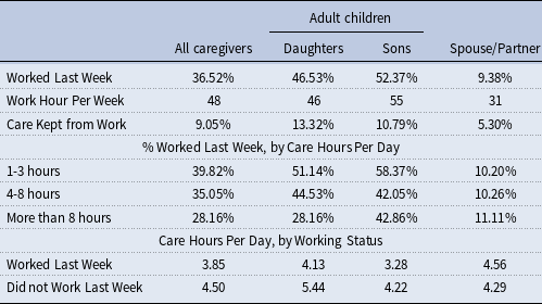
In Table 2, we present the labor supply and caregiving data for unpaid caregivers with known employment status in 2015 NSOC. Around half of the adult-child caregivers worked in the last week, 47% for daughters and 52% for sons. This is comparable to the employment rates for their age and gender groups in the general population. Meanwhile, based on the reported work hours from those that do work, many work full-time jobs (40 hours or more each week). Furthermore, when asked if caregiving has kept them from doing paid work, only 13% of daughters and 9% of all caregivers answered “yes,” meaning that the vast majority of the unpaid caregivers did not feel they worked less as a result of caregiving.
Table 2. Caregiving and employment
Source: 2015 National Study of Caregiving (NSOC). In both tables, “Daughter” includes biological daughter, daughter-in-law, and stepdaughter. Similarly, “Son” includes biological son, son-in-law, and stepson. For the purpose of this paper, we do not distinguish the differences among these subgroups. “Worked Last Week” refers to the fraction of unpaid caregivers that worked for pay in the last week.
We then break down employment status by care intensity, measured in number of care hours per day. Adult-child caregivers who are helping more hours per day are generally associated with lower employment rates. However, we would like to point out that relatively high fraction of caregivers still work while providing care. If we consider caregiving as a job, 4-8 hours a day would be more than some part-time jobs, and more than 8 hours a day is equivalent to or more than a full-time job. This means that while some intensive caregivers had to choose between caregiving and work, more caregivers, including some intensive caregivers, did not, or could not, stop working. We show this from another perspective by breaking the data down by working status. Caregivers who did not work last week provided more care than those that did work. But on average, caregivers who worked are still providing around 4 hours of care a day, which is equivalent to a part-time job.
It is worth noting that a higher number of adult-child caregivers choose to work than spouse caregivers, but provide at least as much care if not more.Footnote 9 Among the adult children, daughters provided more care than sons, and a higher proportion of sons worked than daughters. This is consistent with the empirical findings that women are more likely to be affected by caregiving responsibilities. In conclusion, without claiming causality in any direction between caregiving and employment, we want to emphasize the fact that for most adult children, caregiving and work coexist. The tradeoff happens among work, caregiving, and leisure, not necessarily and exclusively between caregiving and work.
2.4 What motivates adult children to help parents?
To think about how adult children make caregiving decisions, we first think about why adult children help their parents in general. In the theoretical literature on intergenerational transfers, altruism, and bequest expectation are used most often (see Cardia and Michel, Reference Cardia and Michel2004; Mukherjee, Reference Mukherjee2022). Altruism usually means that the well-being of the parent generation is part of adult children’s utility. Both mechanisms indicate that adult children would get something in return for their transfer, utility, or future wealth. We would like to propose a third scenario regarding care-related transfer and refer to it as “need-based altruism.” This altruism motivates children to help parents fulfill their care needs. Parents with means can meet much or all of their needs using the formal care market, while parents with little means rely more on the adult children to provide care. Given the fixed amount of care need, adult children decide how to provide care. The main theoretical difference between the “need-based altruism” and the traditional altruism is that under “need-based altruism," adult children will not help beyond the level of the need, while the traditional altruism will motivate adult children to give until marginal utility becomes small. The latter may be more appropriate describing certain transfer behavior, such as gifting and spending time with parents. But given the nature of caregiving, we think of care-related transfer as a “need-based” decision.Footnote 10
To show some empirical patterns consistent with our suggestion of “need-based altruism," we now turn to the data on time and financial transfers from adult children to parents. Using the 2014 RAND HRS data, we graph the probability and mean of care time and overall financial transfers from children to respondents by parental asset, as shown in Figure 1. We use asset in the old household as a proxy for parents’ ability to fill their own care needs.Footnote 11 Panel (a) shows that parents with relatively low asset are more likely to receive care time and financial transfers from children. Specifically, parents in the lowest quintile are three times more likely to have children giving money to them or caring for them. Panel (b) shows that the magnitude of both types of giving, measured by time and financial transfers from children in the last month, is also negatively related to parental asset.Footnote 12 These results are consistent with our assumption that children with more financially endowed parents face less parental care need, and thus provide less care support.
To sum up this section, we would like to highlight four empirical patterns about elderly care. First, many elders need care, but only a small fraction reside in facilities such as nursing homes. It is common to use unpaid caregivers to assist elders with daily activities, such as grocery shopping and doing laundry. Second, adult children account for more than half of those unpaid caregivers, with majority of them being daughters. They spend a large amount of time caring for parents. The two datasets we looked at show an average care hours of 57 to 66 per month. Third, for adult children caregivers, caregiving and work coexist. Children who provide significant amount of care (more than 8 hours per week) are less likely to be in the labor force, but the overall employment rate among caregivers is high (47%). Fourth, parents in better financial situations receive less care support from children. Specifically, parents in the lowest asset quintile receive more than three times care than those in the highest asset quintile.
Motivated by these empirical findings, we build a theoretical model with the following features. First, elders use a combination of formal care (i.e. nursing home services) and informal care to meet their total care needs. Second, elders use own assets to purchase formal care. If eligible, elders benefit from a government program, similar to Medicaid, and have their care fulfilled through public provision. When private purchase and governmental subsidization are not enough, adult children step in to provide care. Third, children choose time allocation among work, caregiving, and leisure, allowing work and caregiving coexist. We present the details of the model in the next section.

Figure 1. Transfer to parents, by parental assets.
3. Model
We develop a static model formed by a continuum of households. Each household consists of a working-age couple and their retired parent. The working-age couple, or adult children, are the active decision-makers. We choose to study caregiving aside from potential spousal care to focus on the role of adult children, so consider the care need we discuss in this paper as excess care need of the parents that cannot be filled by the spouse. Households are heterogeneous in male and female labor productivity and parental wealth. Our main interest is on women’s caregiving and work decisions, so we allow all men to work full time and carry no care responsibilities. Therefore, the main decision mechanism revolves around the adult daughter’s work and care choices. All households face the same probability of receiving a parental health shock. When shocked, the household needs to arrange care for the parent. This is done through the combination of formal care purchased by the parent or the government from the market and informal care provided by the adult children with time and money. We investigate the heterogeneity in household responses to this health shock and their aggregate effects on the economy.
3.1 Care Production
Each household faces a probability of a health shock,
 $\bar{h}$
. When shocked,
$\bar{h}$
. When shocked,
 $\bar{h}=1$
, the parent loses her ability to perform some daily activities and requires a fixed amount of care,
$\bar{h}=1$
, the parent loses her ability to perform some daily activities and requires a fixed amount of care,
 $H$
. Care is produced as:
$H$
. Care is produced as:
 \begin{equation*}H= s_{i,f} + s_{i,d}\end{equation*}
where
 $s_{i,f}$
is the amount of formal care purchased from the care market, and
$s_{i,f}$
is the amount of formal care purchased from the care market, and
 $s_{i,d}$
is the amount of informal care provided by adult children. For simplicity, we assume these two types of care are perfect substitutes. Informal care requires two inputs from children, time
$s_{i,d}$
is the amount of informal care provided by adult children. For simplicity, we assume these two types of care are perfect substitutes. Informal care requires two inputs from children, time
 $t$
and money
$t$
and money
 $m$
. Time input refers to when children spend their own time caring for parents, such as getting their groceries, taking them to doctor appointments, or simply helping them with household chores. Money input is the cost associated with care provision (i.e. gasoline) and the expenditure on informal care-related services (i.e. ordering food deliveries and paying for house cleaning). We allow the adult children to choose a combination of time and money inputs to highlight how people approach care provision based on their opportunity cost of time. We set a standard c.e.s. home production function for informal care with time and money as inputs:
$m$
. Time input refers to when children spend their own time caring for parents, such as getting their groceries, taking them to doctor appointments, or simply helping them with household chores. Money input is the cost associated with care provision (i.e. gasoline) and the expenditure on informal care-related services (i.e. ordering food deliveries and paying for house cleaning). We allow the adult children to choose a combination of time and money inputs to highlight how people approach care provision based on their opportunity cost of time. We set a standard c.e.s. home production function for informal care with time and money as inputs:
 \begin{equation*}s_{i,d} = \left[\alpha t_i^{\theta } + (1-\alpha ) (\eta m_i)^{\theta }\right]^{1/\theta }\end{equation*}
where
 $\alpha$
and
$\alpha$
and
 $\theta$
are the weight and substitutability parameters, respectively. Parameter
$\theta$
are the weight and substitutability parameters, respectively. Parameter
 $\eta$
acts as a scalar for monetary input. These parameters are important to household decisions when responding to a health shock, and hence we choose their values carefully to reflect observed household behavior in the data. We discuss more details on our approach to set these parameter values in the calibration section.
$\eta$
acts as a scalar for monetary input. These parameters are important to household decisions when responding to a health shock, and hence we choose their values carefully to reflect observed household behavior in the data. We discuss more details on our approach to set these parameter values in the calibration section.
3.2 Labor Market
The economy has a care sector and a non-care sector. All men work full-time in the non-care sector with wages based on their productivity per unit of time,
 $w_{i,m}$
. Women, or adult daughters, choose which sector to work in and how much to work. Let (
$w_{i,m}$
. Women, or adult daughters, choose which sector to work in and how much to work. Let (
 $e_{i,c}$
,
$e_{i,c}$
,
 $e_{i,nc}$
) denote their labor efficiencies in the care and the non-care sectors, respectively. We allow labor efficiencies in the two sectors to be correlated:
$e_{i,nc}$
) denote their labor efficiencies in the care and the non-care sectors, respectively. We allow labor efficiencies in the two sectors to be correlated:
 \begin{equation} ln(e_{i,c}) = ln (e_{i,nc}) + \epsilon _e, \quad \epsilon _e \sim N (0, \sigma _c^2\big) \end{equation}
The market wage rate per efficiency unit of labor in the care sector is
 $w_c$
, which is set in the care sector, separate from that in the non-care sector
$w_c$
, which is set in the care sector, separate from that in the non-care sector
 $w_{nc}$
. This allows us to capture the fluctuations of care market wage, driven by demographic shifts and policy interventions. Women observe the market wage rates in both sectors when making labor supply decisions, and they choose to work in the sector that pays more, so for individual
$w_{nc}$
. This allows us to capture the fluctuations of care market wage, driven by demographic shifts and policy interventions. Women observe the market wage rates in both sectors when making labor supply decisions, and they choose to work in the sector that pays more, so for individual
 $i$
, her wage per unit of time is
$i$
, her wage per unit of time is
 $w_{i,f}=max(w_ce_{i,c},w_{nc}e_{i,nc})$
.
$w_{i,f}=max(w_ce_{i,c},w_{nc}e_{i,nc})$
.
Spousal income is directly correlated to women’s non-care sector labor efficiency. We use the intro-household wage ratios observed in the ACS to pin down spousal wages and discuss this process in detail in the calibration section. We also allow intergenerational wage persistence by linking the non-care sector labor efficiency of the adult daughter and her parent in each household.
3.3 Firms and Output
There are competitive firms producing consumption goods and care service, respectively. Labor is the only input for production in both non-care and care sectors. We normalize the price of consumption goods to 1, and let
 $p$
be the price of care. Firms in the non-care sector face the following problem:
$p$
be the price of care. Firms in the non-care sector face the following problem:
 \begin{equation} \max _{L_{nc}}\pi _{nc} = A_{nc}L_{nc}-w_{nc}L_{nc} \end{equation}
and the competitive nature of the market results in
 $w_{nc} = A_{nc}$
. Firms in the care sector face the following problem:
$w_{nc} = A_{nc}$
. Firms in the care sector face the following problem:
 \begin{equation} \max _{L_{c}}\pi _{c} = pA_{c}L_{c}-w_{c}L_{c} \end{equation}
which results in
 $w_{c} = pA_{c}$
. Therefore, when both markets are in an equilibrium,
$w_{c} = pA_{c}$
. Therefore, when both markets are in an equilibrium,
 \begin{equation*}\frac {w_c}{w_{nc}}=\frac {pA_c}{A_{nc}}\end{equation*}
which shows that the relative wage in the care sector is proportional to the care price.
Total output in the economy is the summation of consumption goods and care services,
 \begin{equation} Y=A_{nc}L_{nc}+pA_{c}L_{c}. \end{equation}
3.4 Government
In the USA, besides the parents themselves, some health insurers also pay for formal care. In the case of Alzheimer’s disease, a progressive chronic condition that requires long-term and potentially intensive care, public insurers, mostly Medicaid, pays more than 70% of formal LTC expenditure in 2013 (Chandra et al. Reference Chandra, Coile and Mommaerts2023).Footnote 13 In our model, care refers to the general care elder parents could use as they age, and LTC would be an important component. So it is necessary for us to acknowledge and include the role public programs play in providing care in an aging population. For simplicity, we model a public care program that mimics Medicaid, which helps pay for formal care for eligible parents. If eligible, this program would fulfill the total care need of the parent. Specifically, if one’s wage is below the wage threshold set by the program, this public care program kicks in and purchases
 $H$
units of care from the market on behalf of the parent.Footnote 14 In other words, for parents covered by this program, their households no longer have care needs to fill. The program is funded by income taxes, and the government runs a balanced budget. For households,
$H$
units of care from the market on behalf of the parent.Footnote 14 In other words, for parents covered by this program, their households no longer have care needs to fill. The program is funded by income taxes, and the government runs a balanced budget. For households,
 $j$
, with parents who are eligible for Medicaid:
$j$
, with parents who are eligible for Medicaid:
 \begin{equation} \tau Y = \sum _{j} pH. \end{equation}
3.5 Agents’ problems
Adult children are the main decision-makers in our model. They face a time constraint across work,
 $n$
, care,
$n$
, care,
 $t$
, and leisure,
$t$
, and leisure,
 $l$
.Footnote 15 Care time is 0 when they do not experience a parental health shock. If the household receives a health shock (
$l$
.Footnote 15 Care time is 0 when they do not experience a parental health shock. If the household receives a health shock (
 $\bar{h}=1$
), parents need
$\bar{h}=1$
), parents need
 $H$
units of care. In this case, the parent checks her Medicaid eligibility first. If she is eligible (
$H$
units of care. In this case, the parent checks her Medicaid eligibility first. If she is eligible (
 $\overline{w_i} \lt W$
), the public program purchases all the care needed. If the parent is not eligible, she spends a fixed proportion of her endowment,
$\overline{w_i} \lt W$
), the public program purchases all the care needed. If the parent is not eligible, she spends a fixed proportion of her endowment,
 $\psi$
, to purchase care,
$\psi$
, to purchase care,
 $s_{i,f}$
.Footnote 16 When her need is not fulfilled through the formal care she purchased for herself (
$s_{i,f}$
.Footnote 16 When her need is not fulfilled through the formal care she purchased for herself (
 $s_{i,f} \lt H$
), adult daughters would provide informal care,
$s_{i,f} \lt H$
), adult daughters would provide informal care,
 $s_{i,d}=H-s_{i,f}$
, to fill the gap. Adult children’s problem can be described as:
$s_{i,d}=H-s_{i,f}$
, to fill the gap. Adult children’s problem can be described as:
 \begin{equation} \max \limits _{n_i,t_i,m_i} ln(c_i) + \nu ln(l_i) \end{equation}
subject to
 \begin{align*} & n_i + t_i + l_i = 1 \\ & c_i + m_i = ( w_{i,f} n_i + w_{i,m}*0.4 ) (1-\tau ) \\ & \left[\alpha t_i^{\theta } + (1-\alpha ) (\eta m_i) ^{\theta }\right]^{1/\theta } = \begin{cases} H-s_{i,f} &\text{ if }\bar{h}=1, s_{i,f} \lt H, \text{ and }\overline{w_i} \geq W\\ 0 &\text{if else}\\ \end{cases} \end{align*}
 $0.2 \le n_i \le 0.4, \quad c_i, l_i, t_i \geq 0.$
Footnote 17
$0.2 \le n_i \le 0.4, \quad c_i, l_i, t_i \geq 0.$
Footnote 17
4. Calibration
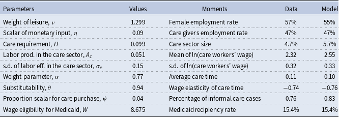
We choose parameter values in the model to form a baseline economy that matches the U.S. data. Some parameters have empirical counterparts, so we estimate their values with labor market and time transfer data. Table 3 reports our estimates. The rest of the parameters are somewhat unique to our model, and we choose their values so that the model generates statistics and patterns that are consistent with the data. We present these parameters and their corresponding moments in Table 4.
Table 3. Exogenously estimated parameters

Table 4. Endogenously estimated parameters
4.1 Exogenous parameters
The first four rows in Table 3 show the parameters we use to generate the wage structure in the non-care sector. We use wage data from the 2007 ACS to create the labor efficiency distribution of women in the non-care sector.Footnote 18 To generate spousal wages, we determine the intra-household wage ratios from the wages of married couples in the ACS, and then produce estimates of
 $\beta _1$
and
$\beta _1$
and
 $\beta _2$
in the following regression:
$\beta _2$
in the following regression:
 \begin{equation} ln\left(\frac{w_{i,m}}{w_{i,f}}\right) = \beta _1 + \beta _2 ln(w_{i,f}). \end{equation}
Using the generated female wages,
 $w_{i,f}$
, and the estimates of
$w_{i,f}$
, and the estimates of
 $\beta _1$
and
$\beta _1$
and
 $\beta _2$
from the regression, we calculate the spousal wages for each household in the model.
$\beta _2$
from the regression, we calculate the spousal wages for each household in the model.
In our model, due to intergenerational wage persistence, children with higher wages tend to have parents with more financial resources. Those children, on average, bear less care burden because we assume parents spend a fixed amount of income on care. We model persistence in labor efficiency between the parent and children generations as follows:
 \begin{equation} ln(e_{i,nc}) = \rho _1+ \rho _2 ln(\overline{e_{i,nc}})+ \epsilon _d, \quad \epsilon _d \sim N \left(0, \sigma _d^2\right) \end{equation}
where
 $\bar{ }$
represents the parent generation within the household. The fifth to seventh parameters in Table 3 govern this persistence. Based on the empirical work by Grawe (Reference Grawe2004), we set the labor efficiency persistence parameter,
$\bar{ }$
represents the parent generation within the household. The fifth to seventh parameters in Table 3 govern this persistence. Based on the empirical work by Grawe (Reference Grawe2004), we set the labor efficiency persistence parameter,
 $\rho _2$
, to 0.47. Conditional on this choice, the constant term,
$\rho _2$
, to 0.47. Conditional on this choice, the constant term,
 $\rho _1$
, and the standard deviation of efficiency shocks,
$\rho _1$
, and the standard deviation of efficiency shocks,
 $\sigma _d$
, are set at values so that women’s wage distribution is stable across generations and follows the same distribution as the data.
$\sigma _d$
, are set at values so that women’s wage distribution is stable across generations and follows the same distribution as the data.
The probability of a parental health shock is set to the fraction of 2015 NHATS respondents who have difficulty with at least one iADL. This is the population of our interest who require regular help from others. We apply the shock probability of 22% uniformly across the population.
4.2 Endogenous parameters
We use nine targeted moments to discipline the remaining nine parameters, as presented in Table 4. While all the nine parameters affect all the moments simultaneously, each moment is most sensitive to a particular parameter, so we will discuss them in pairs.
The first two moments describe the female employment status. The overall female employment rate is calculated using the 2007 ACS data. The weight of leisure in the utility function,
 $\nu$
, reflects the general attitude toward work and helps target the overall employment rate of 57%. In the empirical section, we show that while providing care affects some daughters’ availability to work, many stay in the labor force. We calculate and target the employment rate of caregivers, 47%, using employment status reported by NSOC caregivers. The scalar of adult daughter’s monetary input in the care production function,
$\nu$
, reflects the general attitude toward work and helps target the overall employment rate of 57%. In the empirical section, we show that while providing care affects some daughters’ availability to work, many stay in the labor force. We calculate and target the employment rate of caregivers, 47%, using employment status reported by NSOC caregivers. The scalar of adult daughter’s monetary input in the care production function,
 $\eta$
, is closely and positively related to this moment. As
$\eta$
, is closely and positively related to this moment. As
 $\eta$
increases, monetary input becomes more productive relative to time input, which results in less use of own time for care and leaves more daughter caregivers in the labor force.
$\eta$
increases, monetary input becomes more productive relative to time input, which results in less use of own time for care and leaves more daughter caregivers in the labor force.
We proceed to the next three moments that capture the size and pay of formal care. According to 2007 ACS, 4.7% of employed female work in the care sector. We include people working in the following occupations as care workers: nursing, psychiatric, and home health aides (ACS occupation code 3600), personal and home care aides (ACS occupation code 4610), and personal care and service workers (ACS occupation code 4650).Footnote 19 This employment share partly depends on the total need for care, thus we use the care requirement,
 $H$
, to target this moment. The next two moments are from the 2007 ACS as well, and they capture the wage distribution of care workers. As implied by equation (3) in the firm’s problem, the wage per efficiency unit of labor in the care sector,
$H$
, to target this moment. The next two moments are from the 2007 ACS as well, and they capture the wage distribution of care workers. As implied by equation (3) in the firm’s problem, the wage per efficiency unit of labor in the care sector,
 $w_c$
, is proportional to the care labor productivity,
$w_c$
, is proportional to the care labor productivity,
 $A_c$
. Therefore, we use this parameter to target the mean wage of care workers. We also calculate care workers’ wage variance and use the variance in care efficiency shock,
$A_c$
. Therefore, we use this parameter to target the mean wage of care workers. We also calculate care workers’ wage variance and use the variance in care efficiency shock,
 $\sigma _e$
, to target this moment.
$\sigma _e$
, to target this moment.
The next two moments are related to the care time provided by adult daughters. We limit the NSOC sample to daughter caregivers whose parents have difficulty with at least one iADL (the definition of health shock in the model). We find that the average informal care is 42.45 hours per month, which is 0.11 in the context of the model.Footnote 20 This moment is directly and positively related to
 $\alpha$
, the weight of time input in the informal care production function. The estimated value of
$\alpha$
, the weight of time input in the informal care production function. The estimated value of
 $\alpha$
is 0.77, showing a slightly higher weight of time input relative to monetary input when daughters provide care.
$\alpha$
is 0.77, showing a slightly higher weight of time input relative to monetary input when daughters provide care.
The model predicts a negative relationship between adult children’s wage and the amount of care time they offer, through two channels. First, the opportunity cost of care time increases as children’s wage increases, leading to less caregiving by children. Secondly, due to the built-in income persistence within households, children with higher wages tend to have parents with higher savings. This reduces the care burden on children after parental purchase of formal care, resulting in less informal care needed from children. This pattern between children caregivers’ wage and their caregiving time is consistent with what we find in the data using the 1994 Parent Module in the HRS.Footnote 21 We report the average care time within each wage quartile in Table 5 and show the negative correlation between care hours and the caregiver’s wage. Using this information, we also calculate the caregiver’s wage elasticity of care time to be –0.74. To target this moment, we use the substitutability parameter,
 $\theta$
, in the care production function. When
$\theta$
, in the care production function. When
 $\theta$
is high, time input is more substitutable by monetary input, and children with higher wages are more likely to spend money versus own time in the production of informal care, leading to a steeper negative elasticity. Our estimation of
$\theta$
is high, time input is more substitutable by monetary input, and children with higher wages are more likely to spend money versus own time in the production of informal care, leading to a steeper negative elasticity. Our estimation of
 $\theta =0.94$
shows that the two types of care inputs are quite substitutable. Rupert et al. (Reference Rupert, Rogerson and Wright1995) use PSID data to study the household production sector and estimate the substitutability between home consumption and market consumption goods, similar to our care time and care spending by children.Footnote 22 Their estimates of the substitutability parameter, like ours, are sufficiently greater than 0, particularly for married couples.
$\theta =0.94$
shows that the two types of care inputs are quite substitutable. Rupert et al. (Reference Rupert, Rogerson and Wright1995) use PSID data to study the household production sector and estimate the substitutability between home consumption and market consumption goods, similar to our care time and care spending by children.Footnote 22 Their estimates of the substitutability parameter, like ours, are sufficiently greater than 0, particularly for married couples.
Table 5. Care hours for parents in the previous year, by caregiver’s wage quartiles

Source: 1994 Health and Retirement Study (Parent Module), wage estimated from full HRS panel
The last two moments in Table 4 correspond to the formal and informal care usage among households. We use parameter
 $\psi$
to capture the proportion of parental endowment that is spent on care and choose its value to target the usage of informal care.Footnote 23 Barczyk and Kredler (Reference Barczyk and Kredler2019) provide a cross-country overview on LTC provision. Using data from the HRS, they show that informal care plays the most important part in the USA and report that 76% of care receivers use either informal care exclusively or a mix of informal and formal care. An increase in
$\psi$
to capture the proportion of parental endowment that is spent on care and choose its value to target the usage of informal care.Footnote 23 Barczyk and Kredler (Reference Barczyk and Kredler2019) provide a cross-country overview on LTC provision. Using data from the HRS, they show that informal care plays the most important part in the USA and report that 76% of care receivers use either informal care exclusively or a mix of informal and formal care. An increase in
 $\psi$
allows more parental spending on care, which reduces the care burden on children and the fraction of households relying on informal care. Lastly, we use the wage limit parameter on Medicaid eligibility to target the fraction of people receiving benefits from Medicaid. According to 2015 NHATS, 15.4% of its respondents are covered by state Medicaid program.Footnote 24 We use this number as our target and set the wage threshold for Medicaid at 15th percentile of the parental wage distribution.
$\psi$
allows more parental spending on care, which reduces the care burden on children and the fraction of households relying on informal care. Lastly, we use the wage limit parameter on Medicaid eligibility to target the fraction of people receiving benefits from Medicaid. According to 2015 NHATS, 15.4% of its respondents are covered by state Medicaid program.Footnote 24 We use this number as our target and set the wage threshold for Medicaid at 15th percentile of the parental wage distribution.
The baseline calibration implies an equilibrium care price
 $p = 16.2$
and the tax rate
$p = 16.2$
and the tax rate
 $\tau = 0.49\%$
.Footnote 25 We choose these two parameter values simultaneously with all the endogenously estimated parameters above by iterating on the care price until it satisfies the care market-clearing condition, and on the tax rate until it balances the government budget constraint.
$\tau = 0.49\%$
.Footnote 25 We choose these two parameter values simultaneously with all the endogenously estimated parameters above by iterating on the care price until it satisfies the care market-clearing condition, and on the tax rate until it balances the government budget constraint.
4.3 Untargeted moments
In this section, we report and discuss our model results in other dimensions. We check the fitness of the model by comparing our estimates of some untargeted moments with their empirical counterparts.
4.3.1 Medicaid LTC spending/GDP
The tax rate in our benchmark is 0.49%, which is the percentage of GDP used to fund Medicaid. Reaves and Musumeci (Reference Reaves and Musumeci2015) provide an overview of long-term services and supports (LTSS) financing in the USA. Based on the Centers for Medicare and Medicaid Services National Health Expenditure Accounts data, they show that out of the
 $\$$
310 billion national spending on LTSS, 51% is covered by Medicaid. We use their numbers and impute the Medicaid LTSS expenditure/GDP to be 0.94%. However, The recipients of LTSS include elderly and non-elderly people (i.e. adults and children with physical and mental disabilities), therefore the estimate from Reaves and Musumeci (Reference Reaves and Musumeci2015) is substantially larger than ours. Barczyk and Kredler (Reference Barczyk and Kredler2019) use the OECD 2017 data and show that Medicaid spending on long-term elderly care accounts for 0.5% of GDP. Our spending/GDP ratio is more in line with their estimate.
$\$$
310 billion national spending on LTSS, 51% is covered by Medicaid. We use their numbers and impute the Medicaid LTSS expenditure/GDP to be 0.94%. However, The recipients of LTSS include elderly and non-elderly people (i.e. adults and children with physical and mental disabilities), therefore the estimate from Reaves and Musumeci (Reference Reaves and Musumeci2015) is substantially larger than ours. Barczyk and Kredler (Reference Barczyk and Kredler2019) use the OECD 2017 data and show that Medicaid spending on long-term elderly care accounts for 0.5% of GDP. Our spending/GDP ratio is more in line with their estimate.
4.3.2 Usage of formal and informal care
Barczyk and Kredler (Reference Barczyk and Kredler2019) compare care arrangements across countries and show that people in the USA, similar to those in Southern European countries (i.e. Italy and Spain), rely heavily on informal care. Their estimates show that 64% of care cases use informal care primarily and 24% of care cases use formal home care or nursing home care. We present the fraction of each type of care arrangement in the population from Barczyk and Kredler (Reference Barczyk and Kredler2019) next to the results from our model in Table 6.
Table 6. Care arrangements (%)

Note: Barczyk and Kredler (Reference Barczyk and Kredler2019) count the cases with more than 80% of total care hours being informal as “informal care” and the cases with less than 20% of care hours being informal as “formal care." All other cases fall in the category of “mix IC and FC." We adopt the same rules for categorization.
Our estimates in the benchmark follow a similar pattern as Barczyk and Kredler (Reference Barczyk and Kredler2019)’s empirical findings. The majority of the households with care need rely on informal care. Note that our formal care fraction is lower than Barczyk and Kredler (Reference Barczyk and Kredler2019). This is partly due to our setup that private care spending is a fixed proportion of parental endowment. We choose such linear relationship to remain focused on the question at hand, but this simplification underestimates the care spending for rich households and thus the total formal care usage.
4.3.3 Eligibility for medicaid
Medicaid is a means-tested program funded jointly by the federal and state governments. Its eligibility is linked to the Supplemental Security Income program. For LTC coverage, an elderly can be categorically eligible (purely income-based) or medically eligible (income and medical need-based) for Medicaid. There are variations in income thresholds among states. However, according to De Nardi et al. (Reference De Nardi, French and Jones2016), many states use
 $\$$
6,950 as the statuary yearly income limit in 1996. Adjusted for inflation, it is equivalent of
$\$$
6,950 as the statuary yearly income limit in 1996. Adjusted for inflation, it is equivalent of
 $\$$
12,115 in 2022. Based on the state Medicaid policies collected by American Council on Aging in 2022, we find a similar income threshold. We extract the income limits for Medicaid applicants who need help with ADLs for all states, and the average limit is
$\$$
12,115 in 2022. Based on the state Medicaid policies collected by American Council on Aging in 2022, we find a similar income threshold. We extract the income limits for Medicaid applicants who need help with ADLs for all states, and the average limit is
 $\$$
12,561.Footnote 26
$\$$
12,561.Footnote 26
Our calibration exercise pins down a threshold
 $W=\$8.675/hour$
. If working full-time, this wage generates an yearly income of
$W=\$8.675/hour$
. If working full-time, this wage generates an yearly income of
 $\$$
18,044. Clingman et al. (Reference Clingman, Burkhalter and Chaplain2022) report that workers with very low earnings (career-average earnings for 2021 equal
$\$$
18,044. Clingman et al. (Reference Clingman, Burkhalter and Chaplain2022) report that workers with very low earnings (career-average earnings for 2021 equal
 $\$$
14,620) face a replacement rate of 56%. Using this number, a worker at our wage threshold would receive approximately
$\$$
14,620) face a replacement rate of 56%. Using this number, a worker at our wage threshold would receive approximately
 $\$$
18,044
$\$$
18,044
 $\times$
56% =
$\times$
56% =
 $\$$
10,105 in Social Security. Li and Dalaker (Reference Li and Dalaker2022) use data from the 2022 Current Population Survey Annual Social and Economic Supplement (CPS ASEC) and show that for poor individuals (below 125% of the poverty threshold) aged 65 or older, 80.1% of their total income comes from Social Security. The potential total income of the elderly at our eligibility threshold is
$\$$
10,105 in Social Security. Li and Dalaker (Reference Li and Dalaker2022) use data from the 2022 Current Population Survey Annual Social and Economic Supplement (CPS ASEC) and show that for poor individuals (below 125% of the poverty threshold) aged 65 or older, 80.1% of their total income comes from Social Security. The potential total income of the elderly at our eligibility threshold is
 $\$$
10,105/0.801 =
$\$$
10,105/0.801 =
 $\$$
12,615. This shows our choice of eligibility threshold is in the ballpark as the yearly income limits adopted by many states.
$\$$
12,615. This shows our choice of eligibility threshold is in the ballpark as the yearly income limits adopted by many states.
4.3.4 Time allocation of workers
Kydland and Pretnar (Reference Kydland and Pretnar2019) document the time allocation of workers who provide informal care and those who do not. Using data from the 2003-2016 American Time Use Survey (ATUS), they show that caring for another adult leads to 1.22 hours per week less on work and 3.96 hours less on leisure. We compare our estimates of those measures to theirs in Table 7.
Table 7. Time allocation

Note: Informal care in Kydland and Pretnar (Reference Kydland and Pretnar2019) includes care provided to any infirm adult, not just to the elderly. They choose the data point for “adult care” instead of “elder care” for the larger sample size.
Care time is much higher in our benchmark due to our focus on elderly care.Footnote 27 Workers in our model also have lower labor supply than the sample in the ATUS. This is partly because we aim to capture the labor and care decisions of married adult daughters who have old parents, and this subgroup tends to work less than the representative sample in the ATUS. Regarding the effects of informal care on workers’ time allocation, our results are consistent with the empirical pattern shown in Kydland and Pretnar (Reference Kydland and Pretnar2019). While caregiving crowds out both work hours and leisure time, it has a larger impact on leisure. In the next section, we show that work hour response is highly heterogeneous among households, so the decrease from 0.217 to 0.215 in Table 7 does not reflect the trend for all in our model.
5. Benchmark
5.1 Household response
We generate a benchmark economy using parameter values in Tables 3 and 4. Figure 2 shows the impact of parental health shock on adult children households. The x-axis is the highest potential market wage (between care and non-care sectors) for adult daughters, including those who do not work. We see that, in general, the shocked households have lower consumption, leisure, work hours, and utility, though the differences are not uniform. For women with the lowest wages, they do not work regardless of parental shock, and any informal care is provided with time input exclusively, resulting in lower leisure but no change in consumption. For women with higher wages, they use a combination of time and money inputs to meet the care needs, resulting in lower labor supply and lower consumption. This echoes the empirical findings in the literature that people who spend a considerable amount of time providing care are usually less attached to the labor market and have relatively low wages (see Lilly et al. Reference Lilly, Laporte and Coyte2007; Leigh, Reference Leigh2010; Wang, Reference Wang2021). Facing a parental health shock, some low-wage working women drop out of the labor force and split the extra time between care and leisure. This explains the excess leisure among some shocked households, relative to their counterparts, in panel (b). The higher a women’s wage, the more likely her parent is not eligible for Medicaid; with a higher opportunity cost of time, she relies more on monetary input, so the more her consumption and overall utility decrease from a parental health shock.
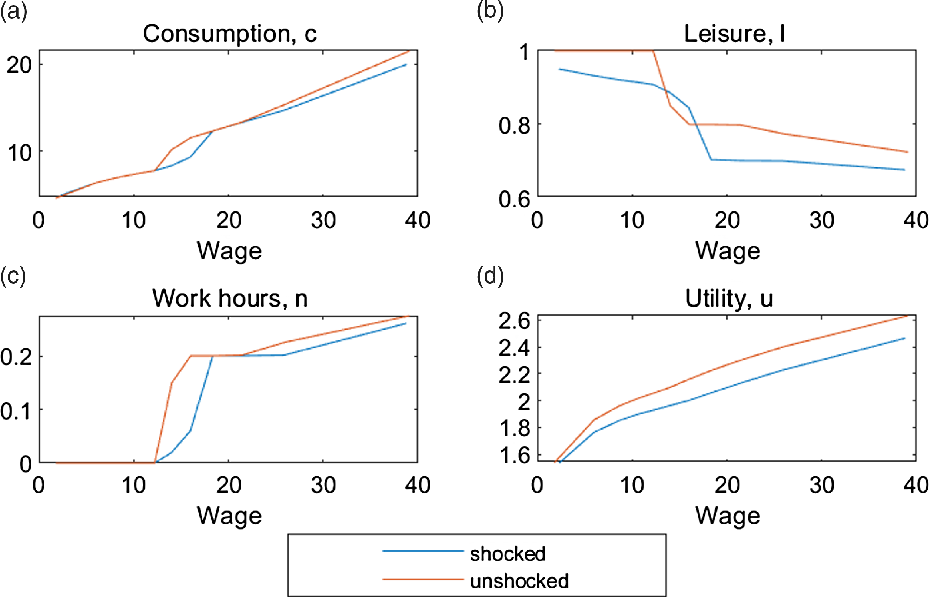
Figure 2. Benchmark household response, by wage.

Figure 3. Benchmark care arrangement, by wage.
Meanwhile, the impact of a parental health shock on leisure is substantial. As we presented in the empirical section, most caregivers in NSOC do not claim that caring for parents hindered their participation in paid work. Our results suggest that much of the consequence of caregiving is a reduction in leisure, rather than in work hours. Kydland and Pretnar (Reference Kydland and Pretnar2019) use the 2003-2016 ATUS data and present the time use differences between caregivers and non-caregivers. Their results show that caregivers cut leisure time (3.96 hours per week) more than work time (1.22 hours per week). Our model generates a similar pattern and further shows a large negative impact on utility.
5.2 Care arrangement
We now look within the shocked households and show how they make care arrangements in Figure 3. Panel (a) shows that the residual care needs from parents, or informal care needs, first increase with children’s wages because the parents are less likely to be eligible for Medicaid, but then decrease with children’s wages because the parents are more able to purchase care themselves. This pattern is confirmed in panel (e), where public spending on care through the Medicaid program decreases and private spending on care through parental purchases increases. As a result, as described in panel (d), formal care use decreases quickly as public spending decreases at first, and then increases slightly as private spending starts to pick up. Regarding the informal care provision, most children rely on own time to give care as panel (b) follows a similar pattern with panel (a). Only children with higher wages use care-related spending to help parents, as shown in panel (c). This tradeoff between the time and money usage in meeting the parental needs is consistent with our model prediction in Appendix A. We then conduct a welfare analysis and show the results in panel (f) of Figure 3. For all affected adult children, we calculate their welfare loss as the percentage decrease in consumption that would lead to the same utility loss caused by the parental health shock. For the households not covered by Medicaid, the welfare loss ranges from 8.3% to 18.9%.
6. Quantitative experiments
We conduct a series of quantitative experiments to explore the impact of the aging population and potential policy interventions. We apply an aged population structure to the model and show the changes in individual household decisions and aggregate measures in the economy. Then, we study how these individual and aggregate outcomes could be amended through three government programs. The first program subsidizes care purchase. The second program expands the existing Medicaid coverage to more parents in need. The third one subsidizes the heavy caregiving adult children with a caregiver allowance.
6.1 Aging population
We are currently experiencing one of the biggest demographic transitions in recent history. According to the Current Population Survey, the mothers of baby boomers had three children on average, whereas the baby boomers themselves had two. This means the children of baby boomers would have, on average, one fewer sibling to share parental care duties with. This can be interpreted as a 50% increase in
 $H$
in our setting.Footnote 28 Consider people aged 18 to 64 as the working-age population and those above 65 as the elderly. In 2007, for each elderly person, there are 5.2 working-age people. According to the population projection from census, by 2060, for each elderly person, there will be 2.4 working-age people. This means that the overall elderly care burden will go up by 115%.
$H$
in our setting.Footnote 28 Consider people aged 18 to 64 as the working-age population and those above 65 as the elderly. In 2007, for each elderly person, there are 5.2 working-age people. According to the population projection from census, by 2060, for each elderly person, there will be 2.4 working-age people. This means that the overall elderly care burden will go up by 115%.
 $^{28}$
Combined with the new
$^{28}$
Combined with the new
 $H$
, we increase the shock probability by 43% to reflect this change.Footnote 29 The top panel of Table 8 shows the changes in these parameter values.
$H$
, we increase the shock probability by 43% to reflect this change.Footnote 29 The top panel of Table 8 shows the changes in these parameter values.
Table 8. Aging population

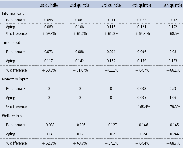
Table 9. Care arrangement, by adult daughters’ wage quintiles
With the adjusted values of
 $H$
and shock probability, our model generates an economy that mimics a more aged population. We report and compare some care arrangement and labor market statistics in the benchmark and the aged economy in Table 8. Informal care needs increase by 63.2%, and this higher need is met by a 62.6% increase in time input and a 79.6% increase in monetary input. The latter is mostly driven by adult children households with high wages. There is a decrease in overall employment from 54.5% to 51.1% as some adult children withdraw from the labor market to provide care. Within this smaller workforce, the employment share of the care sector increases by 91.9%, resulting from the increased need for formal care. This is also reflected in output, where the non-care sector output decreases by 1.8%, while the care sector output increases by 85.3%. Total output decreases by 1% after a larger care sector compensates for nearly half of the decrease in the non-care sector.Footnote 30 Kydland and Pretnar (Reference Kydland and Pretnar2019) find a much bigger negative effect on output due to caregiving in an aging population.Footnote 31 Our model, abstracting from the demographic change in the labor market, is not suited to study aggregate output, but it shows a channel through which the negative impact of caregiving on output can be dampened by the expansion of care sector.
$H$
and shock probability, our model generates an economy that mimics a more aged population. We report and compare some care arrangement and labor market statistics in the benchmark and the aged economy in Table 8. Informal care needs increase by 63.2%, and this higher need is met by a 62.6% increase in time input and a 79.6% increase in monetary input. The latter is mostly driven by adult children households with high wages. There is a decrease in overall employment from 54.5% to 51.1% as some adult children withdraw from the labor market to provide care. Within this smaller workforce, the employment share of the care sector increases by 91.9%, resulting from the increased need for formal care. This is also reflected in output, where the non-care sector output decreases by 1.8%, while the care sector output increases by 85.3%. Total output decreases by 1% after a larger care sector compensates for nearly half of the decrease in the non-care sector.Footnote 30 Kydland and Pretnar (Reference Kydland and Pretnar2019) find a much bigger negative effect on output due to caregiving in an aging population.Footnote 31 Our model, abstracting from the demographic change in the labor market, is not suited to study aggregate output, but it shows a channel through which the negative impact of caregiving on output can be dampened by the expansion of care sector.
To further demonstrate how households are affected by population aging, we present outcomes of adult children who experience a parental health shock by wage quintile in the benchmark economy and in the aging experiment in Table 9. All affected households have higher informal care needs, and thus bear higher time and monetary inputs and welfare losses in an aged economy. Though the increase in parental care needs is uniform, the increase in residual informal care needs is heterogeneous. Households in higher wage quintiles rely more on formal care in benchmark, so when the shock becomes more intense and parents are not able to afford more formal care, they experience a larger change in informal care. Meanwhile, the way adult children provide informal care in the households with time and monetary inputs continues to follow the trend in the benchmark. For households in lower wage quintiles, who rely almost entirely on time input in both scenarios, the increase in time input is proportional to the increase in informal care. For households in higher wage quintiles, because they are more able to use care-related spending to provide care, they choose to disproportionately rely on monetary input. This is shown by the substantial percentage increase in monetary inputs for the 4th (165.4%) and 5th (79.3%) quintile households.
As all affected adult children have to step up to fulfill the extra care needs, welfare loss from the parental health shock increases for all. We notice the largest informal care burden change, an increase of 68.5%, happens to the highest-wage quintile, which translates to the largest welfare loss. This result is partly attributable to our assumption that parents spend fixed amount of money on care, even when care need intensifies. This assumption may be less fair for parents who have more financial flexibility to purchase care and would buy more care in an aged economy, leading to an overestimation of the impact on high-wage households.
6.2 Government policy
In this section, we explore the role of government interventions in an aging population. We first describe how we implement each policy and then compare the impacts of the policies on households and the aggregate economy.
6.2.1 Care services subsidy
We first explore the effects of a care service subsidy that allows parents to buy more care while holding their total care spending constant. Let
 $\gamma$
be the subsidy rate. Formal care purchase by household
$\gamma$
be the subsidy rate. Formal care purchase by household
 $i$
increases from
$i$
increases from
 $s_{i,f}$
to
$s_{i,f}$
to
 $\frac{s_{i,f}}{(1-\gamma )}$
. This subsidy, similar to the Medicaid program, is funded by a flat labor income tax. Therefore, each subsidy rate,
$\frac{s_{i,f}}{(1-\gamma )}$
. This subsidy, similar to the Medicaid program, is funded by a flat labor income tax. Therefore, each subsidy rate,
 $\gamma$
, corresponds to a new labor tax rate,
$\gamma$
, corresponds to a new labor tax rate,
 $\tau _s$
, that allows the program to be budget neutral:
$\tau _s$
, that allows the program to be budget neutral:
 \begin{equation*}\tau _s Y = \sum _{j} pH + \frac {\gamma }{1-\gamma } \sum _{i}(ps_{i,f}) \end{equation*}
where total output and total income,
 $Y$
, are constructed as in equation (4). Households
$Y$
, are constructed as in equation (4). Households
 $j$
are those who are eligible for Medicaid, and households
$j$
are those who are eligible for Medicaid, and households
 $i$
are those that are affected by a parental health shock. For a given subsidy rate, we solve the equilibrium care price and the corresponding tax rate by iterating on them simultaneously until the care market clears and the government budget is balanced. We do this for subsidy rates from 0.1 to 0.5 and graph the results in Figure 4.
$i$
are those that are affected by a parental health shock. For a given subsidy rate, we solve the equilibrium care price and the corresponding tax rate by iterating on them simultaneously until the care market clears and the government budget is balanced. We do this for subsidy rates from 0.1 to 0.5 and graph the results in Figure 4.
The government subsidy program reduces the cost of market care, therefore, households use more formal care and hence, the informal care burden on adult children decreases. This effect is more pronounced for high-wage households as their parents have higher care purchase to start within the benchmark. This is reflected in the bigger impact of higher subsidy rates for these households in Figure 4. We choose the scenario where
 $\gamma =0.2$
,
$\gamma =0.2$
,
 $\tau _s =0.0129$
and compare it to other programs.
$\tau _s =0.0129$
and compare it to other programs.

Figure 4. Household care decisions and care market, by subsidy rate,
 $\gamma$
.
$\gamma$
.
6.2.2 Medicaid expansion
An alternative intervention we explore is an expansion on the eligibility requirement for the Medicaid program. For the ease of comparison across different interventions, we increase the income limit for Medicaid eligibility to the level that the increased tax rate for the subsidy program (
 $\tau _s =0.0129$
) can afford. With such an expansion, now the Medicaid recipiency rate increases from 15.4% to 17.7%. Unlike the subsidy on care purchase that benefits those purchasing more care, who are high-income parents, a Medicaid expansion focuses on poor parents.
$\tau _s =0.0129$
) can afford. With such an expansion, now the Medicaid recipiency rate increases from 15.4% to 17.7%. Unlike the subsidy on care purchase that benefits those purchasing more care, who are high-income parents, a Medicaid expansion focuses on poor parents.
6.2.3 Caregiver allowance
In the last intervention, we designed a program that focuses on adult children with the highest caregiving burden. Medicaid eligibility is based on parents’ income. Due to imperfect income persistence across generations, not all low-income adult children have parents covered by Medicaid. For those who have relatively low wages yet their parents do not qualify for Medicaid, they end up with the largest informal care burden. In this program, we provide an allowance to the top 20% children’s caregivers to compensate for their cost of caregiving time. In the context of our model, these are caregivers whose time input is higher than 0.18, which is equivalent to 17.65 hours a week from a 98-hour week. Keeping the program at the same cost as the other two programs, the allowance is 0.38, which is about 5% of a full-time income at the average wage.
6.3 Comparison and discussion
In Table 10, we present key results for five scenarios: the benchmark, the aged population with no policy intervention, the aged population with each of the three policy interventions, care subsidy, Medicaid expansion, and caregiver allowance. To better compare across scenarios, we normalize public spending in formal care purchase and aggregate outputs in the benchmark to 1. The top half of the table summarizes the changes in assumptions for the scenarios. The main difference across these experiments is how the government engages with care. In the care subsidy program and the Medicaid expansion program, the government interacts directly with the formal care market, by lowering the price of care for households and purchasing extra care, respectively. This increases the average formal care use from 0.038 to 0.041. The caregiver allowance, on the other hand, is relatively small and only for the intensive caregivers whose parents buy very little care, so the program does not affect formal care use.
Table 10. Policy scenario comparison in aged population

In the second half of Table 10, we present some key results from the experiments. First, we look at informal care needs and average time and monetary inputs from adult children. Population aging increases the average informal care needs from 0.068 to 0.111, on top of the increase in formal care from 0.031 to 0.038. The care subsidy and Medicaid expansion programs both cause a shift from informal care to formal care. While having a similar overall effect on informal care, the care subsidy and the Medicaid expansion affect different households. The subsidy has a larger impact on households who buy more care. The adult children in those households are most likely to fulfill care needs with monetary input, so we observe the largest decrease in average monetary input under the subsidy program. Medicaid expansion, on the other hand, affects low-income households, where adult children tend to previously mostly use own time to give care. By lifting the care burden completely from another 2.3% of the population, the Medicaid expansion causes a bigger cut in care time relative to care-related spending. Caregiver allowance, in contrast to the previous programs, has little effects on care provision (formal vs. informal) and informal care production (time vs. monetary input) in our model. A slight decrease in care-related spending comes from the income effect of the higher labor tax that all the adult children are paying to finance the intervention. Care price, endogenous in our model, is higher in an aged population and in the policy scenarios with higher formal care use.
We now look at the implications of the experiments on the aggregate economy. Employment rate increases under care subsidy and Medicaid expansion from an expanded formal care sector, reflected by the larger care output (from 0.018 without intervention to 0.2 with intervention). In all the aged scenarios, non-care output mostly remains unchanged and total output is boosted by the care sector, especially under the care subsidy and Medicaid expansion experiments.
To further understand the welfare impact of these different policy options, we calculate the percentage change in welfare caused by the three interventions and present the results in Figure 5.Footnote 32 Both care subsidy and Medicaid expansion increase welfare, though they have different redistributional effects. The benefit of care subsidy increases steadily with wage whereas Medicaid expansion largely affects households in the lower wage deciles. The caregiver allowance, on the other hand, has quite muted welfare effects in comparison because it does not directly reduce caregiving burden for adult children in our model. For households in the highest-wage decile, who pay a higher labor tax for the program but are not eligible for the allowance, a welfare loss occurs.
Overall, households are more responsive to the subsidy and Medicaid programs, given their direct influence on formal care purchase. Welfare improves under both policies, though the impact varies across households. Designed to directly help informal caregivers, care allowance has minimum effects on household behaviors and their welfare. Potentially, the policy effects could be amplified if we were to reduce the size of the beneficiary group and allow a more generous benefit for eligible caregivers. Still, care allowance would be the most costly way, among all interventions we consider, to provide a relief to caregiving adult children.

Figure 5. Welfare loss comparison.
7. Conclusion
This paper studies the impact of caregiving in an aging population by developing a theoretical model on how elders’ care needs are met. We focus on the decisions of adult children, particularly daughters, in providing informal care using time and monetary input. Our model reveals significant heterogeneity in care arrangements and welfare outcomes across households. We conduct quantitative experiments to shed light on the effects of aging population and three different types of policy interventions. We find that policies that directly reduce the adult children’s caregiving responsibilities through formal care support are the most effective in welfare improvement. Specifically, subsidizing care services is more helpful for households with the financial resources to rely on formal care, whereas expansions on means-tested programs such as Medicaid are more helpful for poor households.
Our model captures several important caregiving patterns observed in the data and provides insights on elderly care burden on adult children. We see the following issues as potential directions for future work. First of all, in order to keep the model tractable and focused on the main mechanism, we abstract from heterogeneity in parental care needs. In our model, parents with a health shock face a fixed amount of care need while elderly care can vary from around-the-clock care to help with grocery shopping. Addressing such variance in care need would provide deeper understanding of how households fulfill care need at different levels. Secondly, our assumption about parental purchase of care (linear to income) underestimates the care spending of rich households. A more sophisticated setup about care expenditure and income would allow a better representation of care provision behaviors of people with more financial resources. Thirdly, the model is largely static because we want to stay focused on the intratemporal interaction between formal and informal care. However, elder caregiving, especially in an aging society, has long-lasting impacts for caregivers, and this feature calls for dynamic models that can capture the effects of care responsibilities over time. We leave these extensions for future research.
Acknowledgments
We thank participants in the 2018 ASSA/AEA CSWEP session on Family and Social Transfers for an Aging Population, Midwest Macro 2018, Liberal Arts Macro 2019, and seminar attendants at Xavier University, Lafayette College and RAND Corporation, for helpful comments. We are grateful for the useful feedback from David Lagakos, Valerie Ramey, Garey Ramey, Claudia Golden, Kathleen Mullen, and multiple anonymous referees. All errors are ours.
Appendix
A. Toy model on intergenerational transfers
We set up the adult children’s household problem to include intergenerational transfers in the simplest way as follows:
 \begin{equation*}\begin{array}{l@{\quad}l@{\quad}l@{\quad}l@{\quad}l@{\quad}l} & \textrm{Traditional Altruism} & & &\textrm{Need-based Altruism} \\ \max \limits_{c, l, t, m} & u_c(c) + u_l(l) + u_h(h(t,m)) & & \max \limits_{c, l, t, m} & u_c(c) + u_l(l) \\ s.t.& n + l + t = 1 & & & n + l + t = 1 \\ & c + m = w n & & & c + m = w n \\ & h = (\alpha t ^ \theta + (1-\alpha) m ^ \theta )^{1/\theta} & & & \bar{h} = (\alpha t ^ \theta + (1-\alpha) m ^ \theta )^{1/\theta} \end{array} \end{equation*}
where
 $c$
is consumption,
$c$
is consumption,
 $l$
is leisure,
$l$
is leisure,
 $w$
is wage,
$w$
is wage,
 $n$
is labor supply, and
$n$
is labor supply, and
 $t$
and
$t$
and
 $m$
are net time transfer and financial transfer to parents, respectively. These two transfers are inputs to a CES production function for parents’ well-being increase from adult children. Note that
$m$
are net time transfer and financial transfer to parents, respectively. These two transfers are inputs to a CES production function for parents’ well-being increase from adult children. Note that
 $h$
is not the general well-being of the parents, but the increase in well-being as a result of the transfers from the adult children so we can abstract from other factors that determine the parents’ well-being. The setup of
$h$
is not the general well-being of the parents, but the increase in well-being as a result of the transfers from the adult children so we can abstract from other factors that determine the parents’ well-being. The setup of
 $h$
is the main difference between the two types of transfer motivation. They are referred to as “traditional altruism” and “need-based altruism." In traditional altruism,
$h$
is the main difference between the two types of transfer motivation. They are referred to as “traditional altruism” and “need-based altruism." In traditional altruism,
 $h$
is a choice variable, whereas in need-based altruism,
$h$
is a choice variable, whereas in need-based altruism,
 $\bar{h}$
is an exogenous variable that can be interpreted as the amount of needs parents have. At any given level of
$\bar{h}$
is an exogenous variable that can be interpreted as the amount of needs parents have. At any given level of
 $h$
/
$h$
/
 $\bar{h}$
, first-order conditions in both household problems will result in an optimal ratio of time and monetary transfer:
$\bar{h}$
, first-order conditions in both household problems will result in an optimal ratio of time and monetary transfer:
 \begin{equation*}\frac {t}{m} = \left(\frac {\alpha }{1-\alpha } \frac {1}{w}\right)^{\frac {1}{1-\theta }}.\end{equation*}
This optimal ratio depends on the relative weight of the two in the production function, the substitutability, and the relative opportunity cost of the two,
 $w$
, where wage is the opportunity cost of time transfer, and 1 unit of consumption is the opportunity cost of monetary transfer. The ratio is positively related to the weight of time inputs and negatively related to wage. This implies that adult children with high wages will depend more on monetary transfer and adult children with low wages will depend more on time transfer.Footnote 33 However, it is important to note that this is only true for a fixed level of
$w$
, where wage is the opportunity cost of time transfer, and 1 unit of consumption is the opportunity cost of monetary transfer. The ratio is positively related to the weight of time inputs and negatively related to wage. This implies that adult children with high wages will depend more on monetary transfer and adult children with low wages will depend more on time transfer.Footnote 33 However, it is important to note that this is only true for a fixed level of
 $h$
. In traditional altruism, the level of
$h$
. In traditional altruism, the level of
 $h$
depends on the marginal utility, as derived from first-order conditions:
$h$
depends on the marginal utility, as derived from first-order conditions:
 \begin{equation*}u^{\prime}_h(h) = u^{\prime}_c(c)/ \frac {\delta h}{\delta m} = u^{\prime}_l (l)/ \frac {\delta h}{\delta t}\end{equation*}
The relationships among the marginal utilities mean that the level of
 $h$
is linked to the levels of
$h$
is linked to the levels of
 $c$
and
$c$
and
 $l$
. Assuming
$l$
. Assuming
 $u_c$
,
$u_c$
,
 $u_l$
, and
$u_l$
, and
 $u_h$
are the utility functions for normal goods, that is, increasing and concave, then households with higher optimal consumption and leisure will choose higher levels of
$u_h$
are the utility functions for normal goods, that is, increasing and concave, then households with higher optimal consumption and leisure will choose higher levels of
 $h$
. In need-based altruism, households would not choose to produce more than
$h$
. In need-based altruism, households would not choose to produce more than
 $\bar{h}$
, that is, they will meet parents’ needs, but not transfer more than that. Then children whose parents have higher needs will transfer more time and money. So in conclusion, wage or relative opportunity cost matters for which type of transfer a household relies on, but the motivation matters for the overall amount of transfer.
$\bar{h}$
, that is, they will meet parents’ needs, but not transfer more than that. Then children whose parents have higher needs will transfer more time and money. So in conclusion, wage or relative opportunity cost matters for which type of transfer a household relies on, but the motivation matters for the overall amount of transfer.
Table A1. Care time from children and parents’ financial status

Standard errors in parentheses
*** p
 $\lt$
0.01, ** p
$\lt$
0.01, ** p
 $\lt$
0.05, * p
$\lt$
0.05, * p
 $\lt$
0.1
$\lt$
0.1
Source: 2014 Health and Retirement Study
Financial transfer amount is measured in thousands of dollars.
B. Extra figures and tables
B.1 Figures on transfers
Figure A1 describes adult children’s transfers to their parents by parental income. The figures show the same pattern where parents in worse financial situations receive more time and financial transfers from their children. Note the outlier point in the second panel. The last observation in the probability panel shows that the parents in the top income quintile are not likely to receive financial transfer (probability less than0.03), but someone who did receive a transfer received a large amount.
B.2 Tables on transfers
Tables A1 and A2 show the regression results on transfers received from the parents’ perspective. In all regressions, we control for parental health status by including a self-reported health score with values ranging from 1 (excellent) to 5 (poor). Ideally, we want to control children’s financial situation in these regressions, but this information, including imputed measures, is limited. We consider different financial status measures (asset, income, and wage) and add various controls. All estimates point to one pattern, parents who are financially better off receive less care time and are less likely to receive financial help from children. In addition, we find that parents who provided financial transfers to children do not receive more care, yet receiving financial transfers from children is an indicator of also receiving more care.
Table A2. Financial transfer from children and parents’ financial status
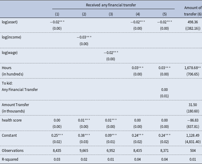
Source: 2014 Health and Retirement Study
“Care hours” refers to the number of care hours the respondent received from all of their adult children last month, measured in hundred hours.
Standard errors in parentheses
*** p
 $\lt$
0.01, ** p
$\lt$
0.01, ** p
 $\lt$
0.05, * p
$\lt$
0.05, * p
 $\lt$
0.1
$\lt$
0.1

Figure A1. Transfer to Parents, by parental income.


 Open access