1 Introduction
How much effect would gaining $500 have on your feelings compared to losing $500? Now, think again. How much effect would gaining 50 cents have on your feelings compared to losing 50 cents? The Nobel prize winning work on valuation of gains and losses in Prospect Theory both for risky (Reference Kahneman and TverskyKahneman & Tversky, 1979Footnote 1; Reference Tversky and KahnemanTversky & Kahneman, 1992) and riskless choices (Reference Tversky and KahnemanTversky & Kahneman, 1991) along with extensive research (for a review, see Camerer, 2005) have suggested a value function where, psychologically, losses loom larger than gains due to a phenomenon called loss-aversion. Although prospect theory was initially concerned with choices and decision utility, Kahneman (1994) later expanded it to the domain of experiences, defining affective judgments about outcomes as predicted utilities and the experiences of outcomes as experienced utility. Irrespective of context, the idea that disutility of losses would always be more intense than gains has been assumed in many theories and models across disciplines (Reference CamererCamerer, 2005; Reference Tom, Fox, Trepel and PoldrackTom, Fox, Trepel & Poldrack, 2007). According to this idea, intensity of affective feelings about the pain of losing exceeds the pleasure of gaining it.
Empirical support for loss-aversion, however, is sketchy. Experiments conducted on choices found loss-aversion to vary across participants, context and magnitude of payoffs (Reference Erev, Ert and YechiamErev, Ert & Yechiam, 2008; Reference Ert and ErevErt & Erev, 2008; Reference Ert and ErevErt & Erev, 2013; Reference Schmidt and TraubSchmidt & Traub, 2002). Other experiments that measured affective judgments either found no loss-aversion (Reference Mellers, Schwartz, Ho and RitovMellers, Schwartz, Ho & Ritov, 1997; Reference Mellers, Schwartz and RitovMellers, Schwartz & Ritov, 1999) or even reversed loss-aversion (Harnick, Van Dijk, Van Beest & Mersmann, 2007). Here we focus on affective judgments that are informative predictors for future choices (Reference Charpentier, De Neve, Li, Roiser and SharotCharpentier et al., 2016; Reference Knutson and GreerKnutson & Greer, 2008; Reference Loewenstein, O’Donoghue and RabinLoewenstein, O’Donoghue & Rabin, 2003; Reference Mellers and McGrawMellers & McGraw, 2001). In fact, one way to look at loss-aversion is to view it as an affective prediction error (Reference Kermer, Driver-Linn, Wilson and GilbertKermer, Driver-Linn, Wilson & Gilbert, 2006; Reference Gilbert and WilsonGilbert & Wilson, 2007). Affect is entwined with the very definition of loss-aversion — “The asymmetry is commonly thought to occur because people expect the pain of losing something to exceed the pleasure of gaining it” (Reference McGraw, Larsen, Kahneman and SchkadeMcGraw, Larsen, Kahneman & Schkade, 2010; pp. 1438). It is hence a problem for the theory if affective judgments are not in agreement with the predicted asymmetry of losses being more intense than gains.
In Harnick et al. (2007), one group of participants rated the affective outcome of small gains while another group rated small losses for the same magnitude in a between-subject design. They used a bipolar scale (–100 to +100) and found that gains loom larger than losses for low magnitudes of money (0.1, 0.5, 1.00, 2.00 euros) but losses loom larger than gains at high magnitudes (50 euros). Other studies like Mellers et al. (1997) presented the gain and loss domain to the same participant in a within-group design but did not find evidence for loss-aversion in judged feelings for gains versus losses for relatively low ranges of money ($16) using a standard bipolar response scale (e.g., –50 for extremely disappointed to +50 for extremely elated). Further, according to the loss-aversion principle, non-losses should be perceived as more positive than gains, but Liberman, Chen, Idson and Higgins (2005) failed to find support for this prediction in judgments of fairness for hypothetical price change scenarios.
McGraw et al. (2010) addressed these deviations from prospect theory’s prediction by suggesting that those studies could not capture loss-aversion in judged feelings due to the method used to measure gains versus losses. Hence, these deviations were suggested to be a measurement issue — not a psychological finding. According to McGraw et al. (2010), a bipolar scale or a between-subject design (both were true for Harnick et al., 2007; Liberman et al., 2005 while Mellers et al., 1997 used a bipolar scale) results in comparing positives with positives and negatives with negatives such that judgments do not cross over the neutral point. Such judgments from two sides (positives with negatives) are then compared later during analysis. These cross valence comparisons do not allow losses to be weighed from a common reference point in comparison to gains. In general, for subjective judgments, within-subject designs provide a common context that is absent or disparate in between-subject studies (Reference BirnbaumBirnbaum, 1999). It was therefore suggested by McGraw et al. (2010) that a unipolar or comparative scale make people judge gains and losses on a similar scale at the same time, and this is necessary for evaluating loss-aversion.
Indeed, McGraw et al. (2010) found significant differences between judged feelings based on the scales used for measurements. A bipolar scale showed no loss-aversion while a unipolar and comparative scale showed loss-aversion. However, McGraw et al. (2010) used a large hypothetical outcome of $200 in their studies, which did not shed light on the question of whether the value function could be magnitude dependent. The question, thus, remained: is reversed loss-aversion (Harnick et al., 2007) or null findings about the asymmetry related to gains and losses (Reference Mellers, Schwartz, Ho and RitovMellers et al., 1997) for small amounts in affective judgments a measurement effect due to response scales and between-subject designs, or is it an actual psychological finding?
The current study addressed this discrepancy with four experiments, which asked whether affective feelings about gains and losses depend on magnitude when people judge gains and losses simultaneously from a common reference point. We used a unipolar (Experiment 1) and a comparative relative-intensity scale (Experiment 2, 3a and 3b) to test the scale-related measurement explanation suggested by McGraw et al. (2010), and we also measured intensity of gains and losses within the same subject. No anchors were provided in Experiments 1 and 2. Experiments 3a and 3b asked whether loss-aversion could disappear even for higher magnitudes if presented with a relatively larger anchor.
2 Experiment 1: Judging prospective small gains and losses for gambles on a unipolar scale
2.1 Method
2.1.1 Participants
A request to participate in a web survey was posted on a popular social media site. The study purported to measure how people might feel about gains and losses. We pre-decided to have about 55–60 participants and a within subject design to achieve a higher power than previous studies (Harnick et al., 2007; Reference McGraw, Larsen, Kahneman and SchkadeMcGraw et al., 2010). The study was conducted on an Indian sample, which was not represented in the previous studies on small gains or losses. Participation was purely voluntary and no compensation was paid. Demographic details were asked at the end of the study. After sixty participants from a range of backgrounds and income groups (Mage = 24.78, SD = 7.22; 22 females; mean monthly income = 31,146.66 INR, SD = 34,506.34) agreed to participate and completed the study, the survey was closed.
2.1.2 Procedure
Participants were asked for affective judgments regarding possible gains and losses ranging from 5 INR to 500 INR. According to purchase parity at the time of this study, USD $2 would buy eatable goods worth about 40 INR in India. In both absolute and relative terms, 5 INR is a small amount and 500 INR is a comparatively larger amount among the range of monetary amounts used.
The study used a 2 (domain: gain versus loss) x 8 (magnitude of amounts in INR: 5, 10, 25, 50, 75, 100, 250, 500) factorial design with both variables manipulated within subjects. All amounts were presented in the same page to present the whole range of values to the participant. The order of presentation of the amounts on the page was randomized separately for each participant. Following the method of McGraw et al. (2010), participants were introduced to a hypothetical game where they could either win or lose money. They were asked to imagine playing such a game that comprised of a number of rounds. Each round would have a 50% chance of gaining a pre-fixed amount of money and 50% chance of losing the same amount of money depending on a coin toss. Thus, probability was not manipulated and expected value of all such gambles was zero (only magnitude was manipulated). As an example, they were told that for a round where 20INR was selected as the amount, they had a 50% chance of gaining 20INR (if the coin lands on heads) and a 50% chance of losing 20INR (if the coin lands on tails). It was also explicitly mentioned that gaining would entail receiving and losing would entail paying up that amount of money (there was no initial payment made to participants). Their task was to imagine playing different rounds of the lottery game for the pre-fixed amounts. After explaining the game, the following instruction was presented:
“Now imagine you are playing this game. Think how you would feel if you gained a specific pre-fixed amount of money or lost the same amount. If you gain, you shall receive the money and if you lose, you shall have to pay that money. We shall present you with some amounts of money corresponding to rounds in the game. Your task is to think, for the amount of money mentioned, if you gained that amount, how much effect would it have on your feelings/emotions, compared to you losing that amount.”
Thus, they had to rate how they would have felt if they gained or lost each amount. (See the Appendix for examples of response scales.) As in McGraw et al. (2010; study 1a), all participants performed two judgment ratings for each amount: (a) How much would be the effect of gaining ‘x’ INR on their feelings/emotions and (b) How much would be the effect of losing ‘x’ INR on their feelings/emotions using a 5-point unipolar scale (0 = No effect, 1 = Small effect, 2 = Moderate effect, 3 = Substantial effect, 4 = Very large effect). The order of asking about gaining and losing was counter-balanced such that for some participants gains preceded loss while for others loss preceded gain. At the end, some demographic questions including income were posed.
2.2 Results
One participant was removed who gave the same rating for all different amounts. Data were analyzed from 59 participants. Using a general linear model, we performed an Analysis of Variance (ANOVA) on intensity of judged feelings with two factors — domain (gains and losses) and amount (5, 10, 25, 50, 75, 100, 250, 500, treated as labels), as within-subject variables. As Mauchly’s Test of Sphericity was significant, a Greenhouse-Geisser correction was applied. The ratings for different amounts are shown in Figure 1. A main effect of amount was observed F(3.59, 208.75) = 186.37, p < .001, ηp2 = .76. The overall ratings for gains were slightly more than losses (Mgains = 2.64, SD = .10; MLosses = 2.55, SD = .09) but the difference was not significant, F(1, 58) = 2.68, p = .10, partial η2 = .04. A significant interaction between domain and amount was observed, F(4.88, 283.47) = 8.15, p < .001, partial η2 = .12 (Figure 1).
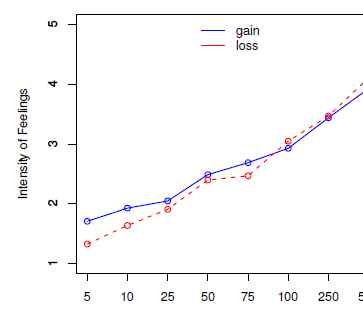
Figure 1: Intensity of gains and losses for different amounts.
To get a clearer idea of the gain and loss difference, for each subject, both the gain and the loss ratings were linearly regressed on the levels of amounts.Footnote 2 Amount was was coded from 5 INR to 500 INR onto 0 to 7 for the eight levels. This enabled us to compare the intercept at 5 INR (i.e., a value of 0) to gauge the difference between gains and losses at this lowest level of magnitude. The individual subject slopes for gains (M = .32, SD = .21) was less than losses (M = .38, SD = .14), t(58) = 2.49, p = .01. Importantly, 0 intercepts calculated for each participant showed a higher value for gains (M = 1.57, SD = .88) compared to losses (M = 1.21, SD = .65), t(58) = 3.83, p < .001 which confirmed that at the lowest point of magnitude (coded as zero), the affective ratings were higher for gains than for losses. The results fit with the Harnick et al. (2007) study even when using a unipolar scale and a within-subject measurement allowing comparative judgment of gains and losses.
To analyze the gains and losses comparatively, we also coded the ratings into three categories as in McGraw et al. (2010). Trials where ratings for gains were greater than losses were coded as ‘1’, gains exactly equal to losses were coded as ‘0’ and losses greater than gains were coded as ‘–1’. This converted the unipolar ratings to a scale akin to the comparative scale. Please note that such an analysis is assuming a conservative null hypothesis of no difference between percentage of participants reporting gains > losses and others reporting losses > gains. For 5 INR (minimum), 64.40% participants stated that gaining versus losing would have the same effect. Among the remaining participants, more people said gains would have more effect than losses for 5 INR (30.50% gains > losses vs. 5.08% losses > gains; sign test p < .001) showing a prominence of gains for low magnitudes. For 500 INR, 61.01% participants stated that gaining versus losing would have the same effect and among others, more people said losses would have more effect than gains (10.16% gains > losses vs. 28.81% losses > gains; sign test p = .005). The percentage of people saying gains would have more effect was clearly more for smaller amounts while those saying losses would have more effect than gains were more for higher amounts when converted to a comparative measurement (Figure 2). A wilcoxon signed-rank test comparing coded ratings on 5INR and 500INR, showed a significant difference, Z = 3.87, p < .001, pointing to the importance of magnitude on ratings of gains or losses. It is important to note that the measurement scales differ a bit. Loss-aversion seemed more noticeable with the transformation to a comparative scale. However, there was no loss-aversion for low magnitudes in both analyses.
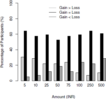
Figure 2: Percentage of participants ratings gain>loss, gain=loss and loss>gain in Experiment 1.
3 Experiment 2: Judging for gambles on a comparative scale
We presented a three-option relative intensity scale (Reference McGraw, Larsen, Kahneman and SchkadeMcGraw et al., 2010; p. 1439) as the response format, which has been argued to be the most effective for capturing loss-aversion.
3.1 Method
3.1.1 Participants
A link to a web survey was sent to a new group of people through messages on social media. After 60 participants from a range of backgrounds (Mage = 27.43, SD = 9.32; 28 females; mean monthly income = 50,008.33 INR, SD = 78,056.06) completed the survey, it was closed.
3.1.2 Procedure
We presented the same scenario as in Experiment 1 and asked participants to judge their feelings for each round of the game. The only difference was the response format. They indicated their feelings about winning a sum of money compared to losing that same amount of money using the following options: (a) gaining would have more effect, (b) losing or gaining would have the same effect and (c) losing would have more effect. The presentation of the ‘gain > loss’ and ‘loss > gain’ options were randomized across participants such that some people were presented with the gain > loss option first while others saw the loss > gain option first and the gain=loss option was always presented in the middle. Participants hence made a single comparative judgment for all amounts (5, 10, 25, 50, 75, 100, 250, 500), presented in different random orders as in Experiment 1.
3.2 Results
We computed the percentage of participants who stated whether for them gains > losses, gains = losses or losses > gains. One participant had not completed the survey; hence data were analyzed from 59 participants. The results clearly showed again that valuation of gains with respect to losses vary with the magnitude of outcomes (Figure 3). An important aspect is that the proportion of people saying gains = losses (or NULL difference) reduced with increases in magnitude using a comparative scale while the proportion remained similar and higher than 50% when a unipolar scale was used (Experiment 1).
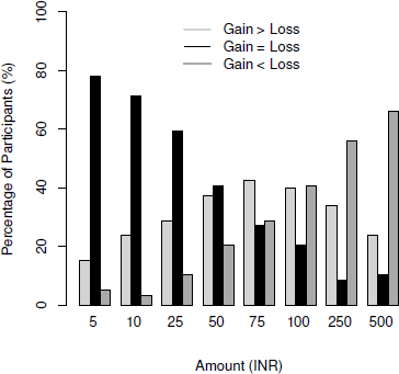
Figure 3: Percentage of participants ratings gain>loss, gain=loss and loss>gain in Experiment 2.
More importantly, for 5 INR, 78.33% participants stated that gaining versus losing would have the same effect and among the remaining ones, somewhat more participants said gains would have more effect than losses (15% gains > losses vs. 6.67% loses > gains; sign test p = .07). For 500 INR, 10% participants said gaining versus losing would have the same effect and among others, significantly more percentage of participants said losses would have more effect than gains (25% gains > losses vs. 65% losses > gains; sign test p < .001). A wilcoxon signed-rank test showed a significant difference in ratings between the low vs high magnitudes of 5 INR vs 500 INR, Z = 3.34, p < .001 that point to the importance of magnitude in influencing comparative valuation of gains and losses. Loss-aversion was observable only for higher magnitudes, while a majority viewed gains and losses similarly (and a few others showed a gain prominence) for lower magnitudes.
4 Experiment 3a: Judging price changes on a comparative scale
This experiment intended to test the previous finding from Experiment 2 in a different context of changing prices. Additionally, we also introduced a high reference point to find how a large anchor influences these judgments. If loss-aversion is contextually dependent on magnitude, a comparatively large anchor should reduce loss-aversion even for higher magnitudes of money.
4.1 Method
4.1.1 Participants
A link to a web survey on ‘thinking about price changes’ was randomly circulated on social media and via email with a request to participate. Fifty-eight participants from different backgrounds (Mage = 26.95, SD = 6.92; 10 females and 11 did not mention gender; mean monthly income = 47,939.13 INR, SD = 71,516.18) responded in a week, after which the survey was closed.
4.1.2 Procedure
The study instructed participants to rate how much effect would either gaining or losing a specific amount of money have for them while purchasing products. We reminded them that in daily life, people often buy products for which there is a decrease in price (gain) or an increase in price (loss). They were asked to imagine going to purchase a product (no specific product was mentioned to remove any effects of prior knowledge) whose price was 5100 INR (as a reference anchor). The task was to think that for a change in price of ‘x’ INR (x = 5, 10, 25, 50, 75, 100, 250, 500 INR presented randomly across participants as before), if they gain that amount because of a decrease in price, compared to another situation where they lose that amount because of an increase in price; what would have more effect on their feelings/emotions? Using a comparative scale, three options were presented: (a) gaining would have more effect, (b) losing or gaining would have the same effect and (c) losing would have more effect, with the order counterbalanced as in Experiment 2. Participants thus made a single comparative judgment for all amounts but for a different context. Additionally, here we presented a reference point of 5100 INR that was 10 times higher than the highest amount of ‘x’ (500 INR) and 100 times higher than the lowest amount (5 INR). This made all amounts comparatively small with respect to the reference price, but at the same time it preserved the relative order of 5 INR being low and 500 INR being high in the range. (See the full questionnaire.)
4.2 Results
One participant was removed who stated a large monthly income and the exact same amount as expenditure (> 3 SD). Responses from 57 participants were analyzed. Figure 4 shows the proportion of participants who stated gains > losses, gains = losses and losses > gains. For the smallest amount (5 INR), 87.71% participants and for the largest amount (500 INR), 7.01% stated that gaining versus losing would have the same effect. Among the remaining ones, there was a slight trend of more participants saying gains would have more effect both for 5 INR (10.52% said gains > losses vs 3.50% stated losses > gains; sign test p = .09) and also for 500 INR (56.14% said gains > losses vs 38.59% stated losses > gains; sign test p = .07). A wilcoxon signed-rank test did not show significant differences between low (5INR) and high (500INR) magnitudes on ratings, Z = –0.83, p = .40.
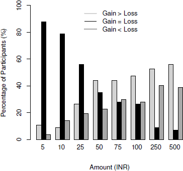
Figure 4: Percentage of participants ratings gain>loss, gain=loss and loss>gain in Experiment 3a.
Similar to Experiment 2, we find that the gain=loss proportion reduces with an increase in amount thus showing that the similar valuation of gains and losses (or NULL differences) reduces as magnitude increases. Unlike Experiment 2, when we presented a higher reference anchor (5100 INR), there was no evidence of loss-aversion both for low and high amounts showing the magnitude-relative nature of loss-aversion.
5 Experiment 3b: Judging for price changes on an extended comparative scale
From the previous experiment, it seemed that a large anchor (5100 INR) removes loss aversion even for higher amounts (500 INR). We wanted to examine the robustness of this pattern in a follow-up experiment. Further, a large percentage of participants stated ‘gain=loss’, especially for small amounts. It is possible that a 3-item comparative scale force people to put most judgments into a big basket of gains=lossesm, or it is possible that indeed the intensity of gains and losses are predicted to be same for small amounts. This experiment thus used an expanded (and hence more sensitive) comparative scale with 5-points to see more into the effect.
5.1 Method
5.1.1 Participants
Fifty-nine participants (Mage = 29.67, SD = 11.14, range = 18 to 53 years; 19 females, 12 did not mention gender; mean monthly income = 76,570 INR, SD = 102,780) responded to an appeal for participating in a web survey on ‘thinking about price changes’.
5.1.2 Procedure
The experimental setup was as in Experiment 3a with only a small addition in the instructions and a change in the response format. To minimize any possible deliberations about purchasing at the slightly higher price level, the following instruction was presented: “Now imagine you going to purchase a product whose price was 5100 Rs. The purchase is one that you have already decided to make, regardless of the price.” Participants had to rate the effect of a gain or loss on a comparative scale where 5 options were presented: (a) Gaining would have a very large effect, (b) Gaining would have a moderately large effect, (c) Gaining and Losing would have the same effect, (d) Losing would have a moderately large effect, (e) Losing would have a very large effect. For half of the participants, the order of the response options was counter-balanced.
5.2 Results
The proportions are shown in Figure 5. For 5 INR, 91.52% participants and for 500 INR, 6.77% stated gains and losses would have the same effect (‘gains = losses’), thus showing that both 3-point and 5-point scales capture similar responses. Like Experiment 3a, the percentage of people stating gains = losses decreased as magnitude increased.
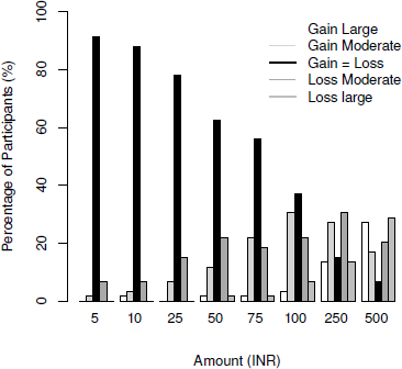
Figure 5: Proportion of participants choosing each of the 5 options in Experiment 3b.
To match the analysis of the former experiments, the percentage of people saying gains would have a very large effect and those saying gains would have a moderately large effect was combined as ‘gains > losses’. Likewise, those saying losses would have a very large effect was combined with those saying losses would have a moderately large effect into ‘losses > gains’. For 5 INR, there was no statistical difference in proportion of people saying ‘losses > gains’ or ‘gains > losses’ as in Experiment 3a (1.69% said gains > losses vs 6.78% stated losses > gains; sign test p = .12). For 500 INR, proportion of people stating gains > losses or losses > gains were almost similar (44.05% said gains > losses vs. 49.14% said losses > gains; sign test p = .67). This confirmed that loss aversion could disappear at both low and high levels of magnitude when one has a comparatively large reference point. Overall, both Experiments 3a and 3b, both point to the magnitude-dependent hypothesis advanced in this paper.
6 General discussion
The current results clear the discrepancy in empirical evidence for affective valuation and shows that for low magnitudes, intensity for predicted gains or losses are similar while at higher magnitudes people may weigh losses more than gains. Moreover, loss-aversion is not observable when one has a large reference anchor. These together suggest that loss-aversion is contextually dependent on magnitude.
The value function of Prospect Theory (slope of the function in particular) needs to be qualified by magnitude’s context effects. McGraw et al. (2010, p. 1443) stated that “at the heart of loss-aversion is a comparison between gains and losses… and when this comparison occurs, losses loom larger than gains”. While the first part of the quotation is justified, the second part is questionable. Experimental results show that losses do not loom larger than gains for low magnitudes of money across all the experiments. On a unipolar scale for hypothetical gamble outcomes (Experiment 1), a reversed loss-aversion was found at very low magnitudes (supporting Harnick et al., 2007) and no differences were found at higher magnitudes (supporting Mellers et al., 1997). Even a comparative scale failed to find losses looming larger than gains for low amounts but did find evidence for losses being more affective than gains at high amounts (Experiment 2). These results suggest that, when stakes are high (for higher amounts), the pain of a negative event looms larger than the pleasure of a similar event but when stakes are low (for lower amounts), the pleasure of a positive event looms larger or equal to the pain of a comparable negative event. A context with a high reference anchor (Experiments 3a and 3b), removed loss-aversion at all magnitudes. While exchanges in the context of prices has been identified as a boundary where loss-aversion is not observed (Reference Novemsky and KahnemanNovemsky & Kahneman, 2005), the combined results in all four experiments show a pattern with gains looming larger or equal to losses for amounts that are low. Thus, there is still ground to cover for understanding the utility of gains and losses along with its implications for theory development (Reference RickRick, 2011).
The valuation process is indeed partly dependent on the measurement scale as suggested by McGraw et al. (2010). From Experiments 1 and 2, we observe that the proportion of people judging gains and losses as equal varied according to the scale, with the unipolar scale showing a fairly similar percentage across magnitudes while the comparative scale reduced that percentage as amounts increased. One reason for that is probably because the comparative scale gives participants more gross categories like gains = losses, gains > losses and losses > gains which forces a comparative judgment to fall in a large category. Note that, simply using a comparative scale will not capture loss aversion as suggested by McGraw et al. (2010). Future research needs to delve more into intricacies of different scales. On the applied side, while labs across the world are using a variety of magnitudes and different measurement scales for behavioral economic experiments, it is vital to consider the influences of such manipulations to correctly interpret conclusions drawn from the studies.
To add to the current results, findings from hedonic forecasts also show that predicted pleasure can be more than predicted pain, moderated by beliefs about likelihood of outcomes (Reference Mellers and RitovMellers & Ritov, 2010). Even for gamble choices, magnitudes are known to moderate people’s choices for low versus high stake gambles (Reference Weber and ChapmanWeber & Chapman, 2005). Magnitude, thus, seems to be a fundamental aspect deciding the properties of the value function in Prospect Theory, beyond some known boundary conditions that influence loss-aversion like affect, age, culture and range of money (e.g., Reference Abdellaoui, Bleichrodt and ParaschivAbdellaoui, Bleichrodt and Paraschiv, 2007; Reference Brooks, Noussair, Capra, Engelmann and BernsBrooks et al., 2010; Reference Mikels and ReedMikels & Reed, 2009; Reference Walasek and StewartWalasek & Stewart, 2015). More generally, although it is a common understanding that affective judgments for ‘bad’ are stronger than ‘good’ (Reference Baumeister, Bratslavsky, Finkenauer and VohsBaumeister, Bratslavsky, Finkenauer & Vohs, 2001; Vasih, Grossman & Woodward, 2008), magnitude of outcomes could be an important moderating factor. The current research shows that it is possible to get different effects based on the amount used, in part explaining the seeming discrepancy in previous literature (e.g., Harnick et al., 2007; Reference Liberman, Idson and HigginsLiberman et al., 2005; Reference McGraw, Larsen, Kahneman and SchkadeMcGraw et al., 2010). While prospect theory probably remains one of the hallmark theories in decision making, mounting evidence suggests a modification in its value function to accommodate differences across low and high magnitudes.
Appendix: Examples of response scales
Unipolar response scale, Experiment 1.
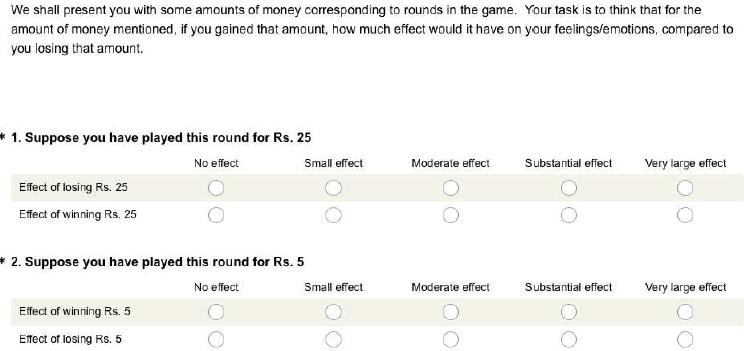
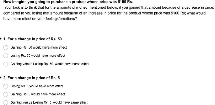
Comparative response scale, Experiment 3a.
