1. Introduction

In order to predict the motion of ice floes, a short-range, small-scale dynamical model has been developed (Neralla and others, in press). In this model ice is considered to move under the action of five forces: the air–ice stress, the water–ice stress, the Coriolis force, the pressure-gradient force due to tilting of the sea surface, and the internal ice stress transmitted through the ice pack. The reasonable agreement of this model with satellite-derived, ice-floe motions demonstrated the feasibility for adoption into the real-time computerized prediction.

In the formulation of ice-dynamics problems, several investigators consider ice as an elastic–plastic material (e.g. Reference Coon, Coon, Maykut, Pritchard, Rothrock and ThorndikeCoon and others, 1974) or viscous-plastic continuum (e.g. Reference HiblerHibler, in press). Following Reference CampbellCampbell (1965), we treated ice as a film of Newtonian highly viscous fluid. In order to arrive at a realistic result we have emphasized the importance of incorporating the variable compactness (fraction of area covered by ice) in the internal ice-stress formulation (Reference Neralla, Neralla, Liu, Venkatesh and DanardNeralla and others, 1977). The aim of this study is to present a simple model to calculate the compactness over a given area.

Reference Nikiforov, Nikiforov, Gudkovich, Yefimov and RomanovNikiforov and others (1967) have used the equation of conservation of mass to study the compactness. The most satisfactory theory incorporating the equation of motion and the equation for conservation of mass has been studied by Reference DoroninDoronin (1970) for summer ice conditions in the Kara Sea. Except in the treatment of air and water stresses, the approach in this study is similar to Doronin’s formulation.

Doronin has also considered sources and sinks terms in the mass equation by taking into account the thermodynamic processes. In our study, we have neglected thermodynamic processes by assuming that mass changes over a period of a few days are small. However, we plan to incorporate them in our future development. In the Arctic Ice Dynamics Joint Experiment (AIDJEX) model (Coon and others, 1974) the mass conservation is obtained by an ice-distribution function.

The study of compactness has several important applications in the Arctic environment. An accurate knowledge of compactness is desirable for more economical and safer navigation and also in the offshore drilling areas, and hence a useful variable in any real-time environmental forecast procedures. In the prediction of an ice-pack front (defined as an edge of a large area of floating ice driven closely together) the internal ice resistance is an important stress which is related to the compactness. A knowledge of compactness is also useful in the vertical heat-exchange computations. The presence of a large concentration of floes inhibits the free movement of icebergs. Hence the study of compactness is important in iceberg grounding problems.

A model for calculating the compactness is discussed in Section 2. This model is applied over the Beaufort Sea area and the results for a few cases are presented in Section 3. Section 4 deals with summary and conclusions of this study.

2. Theory

2.1 General Considerations

In general the compactness C of ice floes obeys

(1)

where V _i is the ice drift and S _i is the sum of the sources and sinks in the given area (e.g. freezing, melting, or precipitation deposited on the ice), and t is the time. Concentration C _N is related to compactness by

(2)

where ρ _i is the density of ice and h _i is the thickness of ice.

The momentum equation for ice floes (Neralla and others, in press) is given by

(3)

where τ _ai is the air–ice stress, τ _wi is the water– ice stress, C _F is the Coriolis force, P_G is the pressure-gradient force due to tilting of the sea surface, and R is the internal ice resistance. Since the area under study is small, we have neglected P _G in Equation (3). Figure 1 illustrates the arrangement of velocities and forces included in the model. For equilibrium, drift equation(3) has been solved by Neralla and others (in press). The internal ice resistance is expressed as

(4)

where K is the horizontal kinematic eddy-viscosity coefficient for ice floes. Campbell (1965) assumed K as constant while Doronin (1970) assumed a realistic form, K ═ K_HC, where K_H is a constant value. Doronin’s relation for K is used here.

Fig. 1. Diagram of force and velocity vectors.

For a single ice floe the internal ice resistance is zero and the momentum equation for equilibrium drift becomes

(5)

which is the equation studied by Reference ShuleykinShuleykin (1938) and Reference ShuleykinReed and Campbell (1962). Shuleykin obtained water currents from the empirical expression of Reference EkmanEkman (1905). Reed and Campbell obtained water currents from the requirements of continuity of mixing lengths and the eddy viscosity at the interface between the boundary and the spiral layers. The solution of Equation(5) is obtained as discussed in detail in Neralla and others (1977). The difference between our method and Reed and Campbell’s method is that the latter assumedV _ai ═ V _a.

2.2. Compactness of Ice Floes

The equations for compactness and momentum in the component form become

(6)

(7)

(8)

where the superscripts x and y denote the x- and y-components.

The solutions of Reed and Campbell’s model (see Equation (5), Section 2.1) as modified by Reference Neralla, Neralla, Liu, Venkatesh and DanardNeralla and others (1977) are used as initial conditions. No slip boundary condition for V _i and no diffusive boundary condition for C are used.

If S denotes the fraction of land area of a grid point, then the maximum value of C is C ═1 when S ═ 0 and C ═ 1—S when S > 0. Table 1 shows the fraction of land area of a grid point. If the compactness at a grid point is less than 0.1, then R is neglected in the computations.

Table 1. Fraction of land area at every grid point over the Beaufort sea

The modified Liebmann successive over-relaxation technique (Reference Carnahan, Carnahan, Luther and WilkesCarnahan and others, [^c1969]) with a projection method to control the non-linear form is applied for solving Equations (7) and(8).

Let (l, m) be the indices of x, y coordinates at a grid point and N the iteration number. The x-component of ice velocity V _i ^x is calculated from

(9)

where

(10)

(11)

(12)

(13)

(14)

(15)

ω is the relaxation factor and and are evaluated by using

(16)

The y-component of ice velocity, V_i ^y is calculated in a similar way.

3. Results

Figure 2 shows the variation of ice drift and deviation angles with wind speed for two sets of air–ice drag coefficients and ice thicknesses representing smooth and thin ice (C_d ^a ═1.4 ×10^–3 and h _i═ 2 m) and rough and thick ice (C_d ^a ═ 2.6 ×10^–3 and h_i ═ 5 m) (Reference Banke and SmithBanke and Smith, 1971). The following values are used for other constants: C_d ^w ═ 3.8×10^–3, ω ═7.29 × 10^–5 s^–1, ρi ═ 0.9 g cm^═3, ρ _a = 1.29 x 10^–3 g cm^–3, ρ_w ═ 1.03 g cm^–3. The ice drifts are in reasonable agreement with other studies (e.g. Shuleykin, 1938; Reed and Campbell, 1962).

The present model is applied for five different cases over the Beaufort Sea area (Fig. 3). It is to be noted here that ice floes are considered to be the rough and thick category (i.e. C_d ^a═ 2.6 × 10^–3, and h_i ═ 5 m). The value used for K_H in this study is 3.3 × 10¹³ g s^–1.

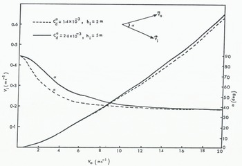
Fig. 2. Variation of ice speed V_i and deviation α with wind speed for two sets of air–ice drag coefficients and ice thicknesses.

Based on the similarity theory approach, Reference AgnewAgnew (1977) developed a model to diagnose surface winds over a grid (Fig. 3). The grid distance in our study is 127 km. We have used this model to obtain surface winds at every 24 h for the period of our interest.

Fig. 3. Diagram showing location of 8 × 8 grid array in the Beaufort Sea.

The observed information on ice compactness was obtained from the subjectively prepared daily ice charts at the Ice Forecasting Central, Ottawa. The required grid-point data are hand-abstracted from these charts.

Five cases have been selected during the period of July and August 1975. After every time step (24 h) new winds are read in. The integrations have been carried out for a period of 5 d. The predicted compactness is verified with observed hand-abstracted data.

Figures 4 to 8 show, for each case, the initial, predicted, and observed values of compactness. With a steady large-scale flow over the area of interest, the agreement of model predictions with observations for cases in late July (Figs 4 and 5) is reasonable. The predicted distribution of compactness (in particular, 0.5 isopleth) in Figures 4 to 7 agrees well with the observed distribution. The model performance for the period 24–29 August 1975 (Fig. 8) is only marginal, presumably due to abrupt changes in winds caused by a fast-moving intense weather system.

Although the predictions agree reasonably well with observations, it would be more realistic to incorporate the sources and sinks term in the continuity equation for compactness. However, the present results from the simple formulation demonstrate the applicability of the technique for short-term forecasting of compactness over a small area.

Fig. 4. Compactness (a) at initial time, 21 July 1975, (b) 5 d forecast valid for 26 July 1975, and (c) observed at 26 July 1975.

Fig. 5. Compactness (a) at initial time, 24 July 1975, (b) 5 d forecast valid for 29 July 1975, and (c) observed at 29 July 1975.

Fig. 6. Compactness (a) at initial time, 15 August 1975, (b) 5 d forecast valid for 20 August 1975, and (c) observed at 20 August 1975.

Fig. 7. Compactness (a) at initial time, 19 August 1975, (b) 5 d forecast valid for 24 August 1975, and (c) observed at 24 August 1975.

Fig. 8. Compactness (a) at initial time, 24 August 1975, (b) 5 d forecast valid for 29 August 1975, and (c) observed at 29 August 1975.

4. Summary and Conclusions

A simple model to calculate the ice drift and compactness of ice floes is presented here. This model is applied over the Beaufort Sea area. Five-day integrations have been carried out using the initial ice-cover data obtained from the daily composite ice charts prepared at the Ice Forecasting Central, Ottawa. The preliminary results of the model are encouraging. For computing compactness over a longer period, thermodynamic processes are important. A further development incorporating these processes is planned.

Since the model is wind driven, reasonably good wind forecasts are required to improve the model performance. The larger grid distance used here may obscure some of the phenomena such as cracks and leads. Reducing the grid size may improve forecasts and also help to explain cracks or narrow leads.