2. CORRECTION OF STRAIN-RATE CALCULATION

The calculation of strain rate is presented by Hutchings and others (Reference Hutchings, Heil, Steer and Hibler2012). Buoy positions, recorded every 10 min, are linearly interpolated hourly. The hourly positions are used to estimate buoy array area and strain-rate (Fig. 1) following a generalisation of the Kwok (Reference Kwok2003) Green's theorem method to use any number of buoys surrounding a deforming region. In Hutchings and others (Reference Hutchings, Roberts, Geiger and Richter-Menge2011) there is a sign error in the calculation of the strain-rate components $\displaystyle{{\partial u} \over {\partial y}}$ and $\displaystyle{{\partial v} \over {\partial y}}$. The correct strain components are calculated as:

(1)$$\displaystyle{{\partial u} \over {\partial x}} = \displaystyle{{1}\over {2A}} \left [ \sum_{n=1}^{N-1}{ (u_ {n+1} + u_n) (y_{n+1} - y_n) } + (u_{1} + u_N) (y_{1} - y_N) \right ],$$

(2)$$\displaystyle{{\partial u} \over {\partial y}} = - \displaystyle{{1}\over {2A}} \left [ \sum_{n=1}^{N-1}{ (u_{n+1} + u_n) (x_{n+1} - x_n) } \!+\! (u_{1} + u_N) (x_{1} - x_N) \right ],$$

(3)$$\displaystyle{{\partial v} \over {\partial x}} = \displaystyle{{1}\over {2A}} \left [\sum_{n=1}^{N-1}{ (v_{n+1} + v_n) (y_{n+1} - y_n) } + (v_{1} + v_N) (y_{1} - y_N) \right ],$$

(4)$$\displaystyle{{\partial v} \over {\partial y}} = - \displaystyle{{1}\over{2A}} \left[ \sum_{n=1}^{N-1}{ (v_{n+1} + v_n) (x_{n+1} - x_n) } + (v_{1} + v_N) (x_{1} - x_N) \right].$$

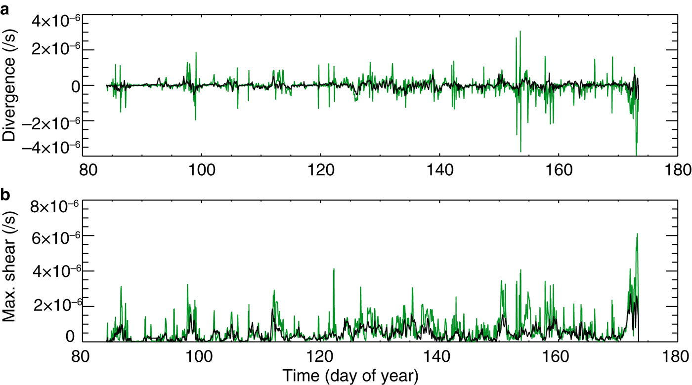
Fig. 1. Corrected Figure 2 in Hutchings and others (Reference Hutchings, Roberts, Geiger and Richter-Menge2011). Time series of divergence rate ($\epsilon_I$) and maximum shear rate ($\epsilon _{II}$) for the 140 km scale array (black) and 20 km scale array (green). Total deformation rate is calculated as $\sqrt {(\epsilon _I^2 + \epsilon _{II}^2)}$.

Note that the right-hand rule applies and we sum in a counter-clockwise direction, around each buoy array of N buoys, to estimate the line integrals.

These strain-rate components are combined to give divergence, vorticity, pure and normal shear as described in Hutchings and others (Reference Hutchings, Heil, Steer and Hibler2012). The maximum shear strain rate is the resultant of pure and normal shear and does not include the factor of a half shown in Hutchings and others (Reference Hutchings, Heil, Steer and Hibler2012).

3. CORRECTED RESULTS

There are subtle differences in several figures resulting from correcting the sign error. These do not affect the interpretation of the data presented in the paper, except in one case. We discuss these differences here.

Figure 2 has a slightly different scaling relationship between total deformation, D, and length scale, L, $D \propto L^{H}$, with H = −0.21 (reported at H = −0.19 in Hutchings and others (Reference Hutchings, Roberts, Geiger and Richter-Menge2011)). There are also small differences in the scaling relationship found for other moments of the deformation (Fig. 3).

Fig. 2. Corrected Figure 3 in Hutchings and others (Reference Hutchings, Roberts, Geiger and Richter-Menge2011). All realisations of deformation rate and length scale (square-root of area), for each sub-array in all sets, are plotted in colours corresponding to the length scales they are grouped into. Mean sub-array length scale and mean deformation is plotted (black stars) for each buoy sub-array set. The least squares fit to these values is shown as a solid line. The variance of deformation for each sub-array is plotted (black crosses) and the dashed line is least squares fit to these points.

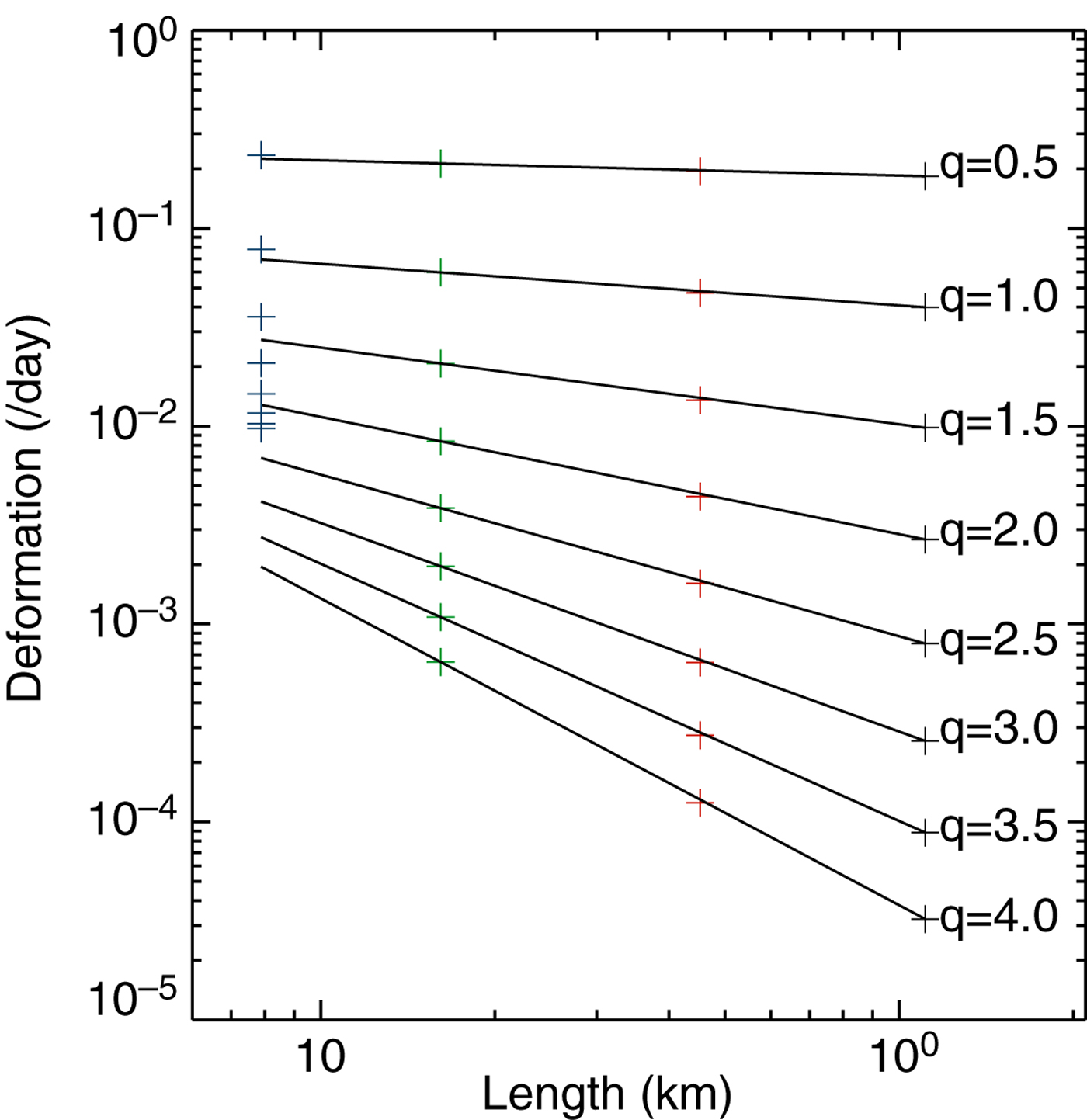
Fig. 3. Corrected Figure 4 in Hutchings and others (Reference Hutchings, Roberts, Geiger and Richter-Menge2011). Moments (q), between 0.5 and 4, of deformation rate (<D^q>), plotted against length scale. The colour of crosses corresponds to length scale as in Figure 2.

We still find a small spread in the timescaling for different length scales (Fig. 4). The spectra of total deformation (Fig. 5) demonstrates a spread of behaviour from white noise for the smallest arrays to close to red noise at the 140 km scale. There is no change to the conclusions in the paper regarding the fractal scaling in time varying across length scales.

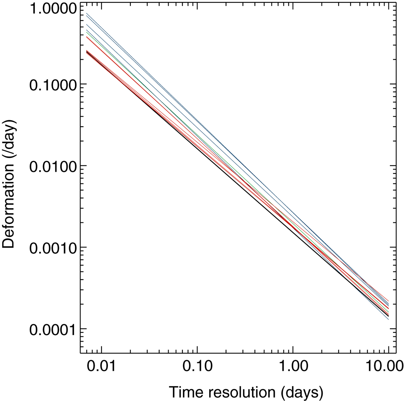
Fig. 4. Corrected Figure 5 in Hutchings and others (Reference Hutchings, Roberts, Geiger and Richter-Menge2011). Least square fit to the means of deformation rate at each timescale sampled for all SEDNA sub-arrays. The colour corresponds to the spatial scale family, the sub-array belongs to: 10 km blue; 20 km green; 70 km red; and 140 km black. The gradients of the smallest arrays are close to −1.1 and the largest array has a gradient of −1.0.

Fig. 5. Corrected Figure 6 in Hutchings and others (Reference Hutchings, Roberts, Geiger and Richter-Menge2011). Spectral density of deformation for each sub-array, and mean log-log linear fit to spectra with spatial scales of 10 km (blue), 20 km (green), 70 km (red) and 140 km (black) are plotted. At the largest spatial scale, 140 km, the spectra can be approximated by red noise. The other spectra are pink, becoming whiter as spatial scale decreases. At the largest spatial scale, 140 km, the spectra has a slope of −1.97, and this slope decreases with reducing spatial scale: −1.76 (70 km), −1.44 (20 km) and −1.36 (10 km).

In spectra of divergence (not shown) a semi-diurnal peak is now apparent. Whereas this does not affect the results presented in this paper, it could have implications to readers interested in sub-diurnal motion of the pack in the Beaufort Sea.

The change in gradient of the fit line in Figure 6 is due to the higher scaling exponents at smaller timescales. The linear relationship between space and timescales holds true, as reported before. This relationship when extrapolated to the timescales represented by RADARSAT satellite overpasses, typically 1–3 days, gives H values between −0.16 and −0.19. Previous work using RADARSAT ice-deformation data identified H to be −0.18 (Marsan and others, Reference Marsan, Stern, Lindsay and Weiss2004). Our correction brings our results further in line with previous observations, as the scaling exponent for 1 h deformation is no longer the same as that for the 1–3 day sampling of RADARSAT. This lends confidence to the finding that we can relate the scaling relationships to the temporal scale with a linear relationship in the mean.

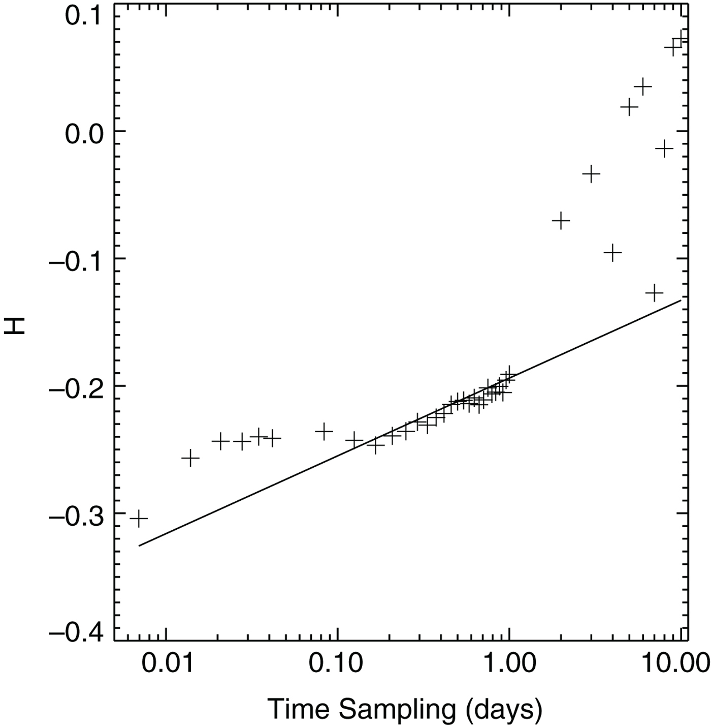
Fig. 6. Corrected Figure 10 in Hutchings and others (Reference Hutchings, Roberts, Geiger and Richter-Menge2011). Gradients calculated as in Figure 2, for time sampling that varies between 10 min and 10 days. A least square fit to values of H and log(T) is shown. The gradient of this fit is $0.6\, {\rm log day^{-1}}$.

Finally, cross correlation between the divergence of the small, inner and large, outer buoy arrays (Fig. 7) displays similar patterns to those reported in Hutchings and others (Reference Hutchings, Roberts, Geiger and Richter-Menge2011). As before, up until June sea-ice deformation displays coherent deformation between 100 km and the scale of the Beaufort Sea (of order 1000 km) over synoptic time periods. We do find one change: there is no longer a loss of coherence around mid-May. This revised result suggests the transition to a spring ice pack when connectivity is reduced, is occurring in June rather than May and, thus, is happening later and more abruptly than previously shown. The semi-diurnal peak in divergence is increased in the new results, with enhanced coherence on this time period.

Fig. 7. Corrected Figure 11 in Hutchings and others (Reference Hutchings, Roberts, Geiger and Richter-Menge2011). The coherence between wavelet spectra of divergence time series for small, 20 km, and large, 140 km buoy arrays. 95% significance levels are encircled by solid black lines. The cone of influence is shown with a bold solid white line, regions outside of this cone indicated by vertical dashed white lines contain data that is likely unrepresentative. 0000Z on 1 May and 1 June are indicated by their month.